Direct numerical simulation of cylindrical particle-laden gravity currents

Open Archive TOULOUSE Archive Ouverte (OATAO)

OATAO is an open access repository that collects the work of Toulouse researchers and

makes it freely available over the web where possible.

This is an author-deposited version published in :

http://oatao.univ-toulouse.fr/

Eprints ID : 14449

To link to this article : DOI :

10.1016/j.compfluid.2015.09.001

URL :

http://dx.doi.org/10.1016/j.compfluid.2015.09.001

To cite this version : Zgheib, Nadim and Bonometti, Thomas and

Balachandar, Sivaramakrishnan

Direct numerical simulation of

cylindrical particle-laden gravity currents

. (2015) Computers and

Fluids, vol. 123. Pp. 23-31. ISSN 0045-7930

Any correspondance concerning this service should be sent to the repository

administrator:

staff-oatao@listes-diff.inp-toulouse.fr

Direct numerical simulation of cylindrical particle-laden gravity currents

N. Zgheib

a,b

_{, T. Bonometti}

b,c

_{, S. Balachandar}

a,∗

a_{Department of Mechanical and Aerospace Engineering, University of Florida, Gainesville, FL 32611,USA}

b_{Université de Toulouse, INPT, UPS, IMFT (Institut de Mécanique des Fluides de Toulouse), UMR 5502, Allée Camille Soula, F-31400 Toulouse, France} c_{CNRS; IMFT; F-31400 Toulouse, France}

Keywords:

Direct numerical simulations Particle-laden flow Turbidity currents

a b s t r a c t

We present results from direct numerical simulations (DNS) of cylindrical particle-laden gravity currents. We consider the case of a full depth release with monodisperse particles at a dilute concentration where particle–particle interactions may be neglected. The disperse phase is treated as a continuum and a two-fluid formulation is adopted. We present results from two simulations at Reynolds numbers of 3450 and 10,000. Our results are in good agreement with previously reported experiments and theoretical models. At early times in the simulations, we observe a set of rolled up vortices that advance at varying speeds. These Kelvin–Helmholtz (K–H) vortex tubes are generated at the surface and exhibit a counter-clockwise rotation. In addition to the K–H vortices, another set of clockwise rotating vortex tubes initiate at the bottom surface and play a major role in the near wall dynamics. These vortex structures have a strong influence on wall shear-stress and deposition pattern. Their relations are explored as well.

1. Introduction

Particle driven currents are a special form of gravity currents in which the density difference is caused by the suspension of particles within an interstitial fluid forming the current. If the mixture density of such a suspension is larger than that of the ambient fluid, it will advance primarily horizontally as a turbidity current [12,17]. Turbidity currents are inherently more complex than homogeneous conservative currents because the density of the current (and conse-quently the density difference between the current and the ambient) may vary temporally and spatially as a result of the settling and entrainment of particles. The effective settling speed of particles, for example, may depend on particle Reynolds number, particle flocculation, and interaction with surrounding turbulence. On the other hand, if the current is traveling fast enough over an erodible bed, it may entrain particles causing it to move even faster and consequently entrain more particles in a self-reinforcing cycle.

Particulate gravity currents are observed in many industrial, environmental, and geological situations. Owing to their destructive nature, turbidity currents constitute a major factor in the design of underwater structures such as pipelines and cables[22]. In an industrial context, they are essential for transporting sediments that may contain pollutants. Furthermore, they are responsible for the formation of submarine canyons as well as for sedimentation transport into the deep oceans.

Particulate constant volume releases[1–3,6,12,14,18]have been studied. However, these finite releases are invariably dominated by fronts. Often in turbidity currents, it is very important to look at the body of the current after the head had long moved away. Experimental and computational investigation of the body is some-how harder and is usually investigated through constant flux cur-rents[11,16,20,23]. In the present context, we explore a finite-volume cylindrical release of particle-laden fluid in clear ambient surround-ing. We wish to identify the dynamics of the current, specifically the three-dimensional propagation and vortical structures of the current. Here we are only concerned with deposition and neglect the effects of resuspension. In reality, resuspension of particles may play a role, but the mechanisms of re-suspension are not fully understood and models of resuspension rate remain empirical with large uncertain-ties (see[26]). In order to make the problem simple and manageable, we look only at the problem of deposition.

Predicting the deposition pattern or the sediment erosion re-sulting from a turbidity current necessitates a good understanding of the mechanism of sediment transport and particle deposition, which are highly dependent on the dynamics of the current, the level of turbulence, and the fluid-particle interaction. As a result, a great level of simplification is generally taken, usually through depth averaging, when studying particulate-driven currents. Some of the models include the Box Model[2,9], which is a simple and fast way to model the extent, speed, and sedimentation rate of turbidity currents. The Box Model is not directly derived from the Navier–Stokes equations; however, it considers the current to evolve with negligible entrainment through a series of height diminishing concentric cylinders for an axisymmetric lock release configuration. In addition to depth averaging, no radial variation is allowed.

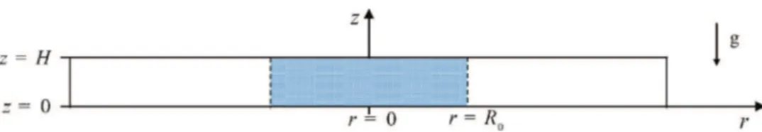
Fig. 1. Side view of the initial setup of the cylindrical lock-exchange flow inside a rectangular box of size Lx×Ly×H = 30 × 30 × 1. Initially, a cylindrical gate of radius R0=2 placed at the center of the domain separates particle-laden fluid from the ambient clear fluid. Once the gate is lifted, the simulation starts and the particle-laden fluid begins to intrude horizontally into the ambient.

A more complex model is based on the Shallow Water equations [3,24,8], which are derived by vertically averaging the Navier–Stokes equations under the assumption of high length-to-thickness aspect ratio. However, because of the variable volume fraction of the cur-rent, an equation of particle conservation is further required. Such models do not usually account for sediment entrainment on the ba-sis that the velocities are insufficient to lift up particles, however the flow is considered to be sufficiently energetic so that turbulent mix-ing maintains vertically uniform properties.

Most research on axisymmetric particle-laden gravity currents has mainly revolved around the early experiments of Bonnecaze et al. [3]and theoretical models mostly based on the Box Model and Shallow Water equations[24,13]. Our objective in this study is to consider a scenario that is similar to what has been investigated experimentally and examine it through direct numerical simula-tions. Highly resolved simulations for cylindrical density-driven finite-release currents have been investigated in the past with results comparing favorably with experiments[4]. Here we consider direct numerical simulations of particle-laden currents resulting from the release of an initial cylindrical fluid-particle mixture.

The DNS will allow us to explore the three-dimensional struc-tures of the current from iso-surfaces of density and iso-surfaces of the swirling strength that show the intensity and structure of the coherent eddies. In many applications, these large scale vortical structures will play an important role in the erosion and resuspen-sion of particles by locally modifying the shear stress at the bottom wall. They also play an important role in the deposition of particles by transporting low particle concentration fluid (particle-laden current mixed with ambient) from the current’s top layers towards the bottom wall and consequently decreasing the local settling rate. This study will be limited to finite-releases of full-depth cylindrical gravity currents with dilute concentrations of monodisperse parti-cles. The paper is arranged as follows. The mathematical formulation is outlinedSection 2. InSection 3, we present our simulation re-sults and compare, where possible, to previous experimental and theoretical data. Finally, main conclusions are presented inSection 4.

2. Mathematical formulation

A side view of the problem setup is shown inFig. 1. Initially, a cylindrical gate separates a relatively heavier (compared with the am-bient) particle-laden fluid of initial density

ρ

c0=

(ρ

p−

ρ

a

)φ

0+

ρ

ain

its interior from the surrounding clear ambient fluid of density

ρ

a.

Both fluids are initially at the same level and occupy the entire height of the domain (seeFig. 1). Here,

ρ

p represents the density of

sus-pended particles, and

φ

0 is the initial volume fraction occupied by

those particles.

Our focus is to simulate buoyancy driven flows with dilute sus-pensions, where particle-particle interactions may be neglected. We consider monodisperse particles whose size is much smaller than characteristic length scale H of the problem. The particle-laden solution will be treated as a continuum and a two-fluid formu-lation is adopted. We follow Cantero et al. [6]by implementing an Eulerian–Eulerian model of the two-phase flow equations. The model involves (i) mass (ii) and momentum conservation equations

for the continuum fluid phase, (iii) an algebraic equation for the particle phase where the particle velocity is taken to be equal to the local fluid velocity and an imposed settling velocity derived from the Stokes drag force on the particles, (iv) and a transport equation for the volume fraction (particle phase). The non-dimensional system of equations read

∇

·u = 0 (1) Du Dt =

φ

e g₋

_∇

_{p +} 1 Re

∇

2_{u (2)} up=u + us (3)

∂φ

∂

t +

∇

·

(φ

up

)

= 1 Sc Re

∇

2

_φ

₍₄₎

Here eg_{is a unit vector pointing in the direction of gravity. Unless}

otherwise stated, all parameters are non-dimensionalized. The height H of the domain is taken as the length scale, U =

p

g′

0H as the

velocity scale, T = H/U as the time scale,

ρ

aas the density scale, and

ρ

aU2as the pressure scale. The reduced gravitational acceleration is

defined as g′

0=

(ρ

p−

ρ

a

)φ

0g/

ρ

a. We denote by upand

φ

the velocity

and the volume fraction of the particle phase, respectively. u and p correspond to the velocity and total pressure of the continuum fluid phase, respectively. The settling velocity usis determined from the

Stokes drag force on spherical particles with small particle Reynolds numbers. Here, the density of particles is assumed to be appreciably larger than that of the ambient fluid such that the dominant force on the particle is the Stokes drag. The Reynolds and Schmidt numbers inEqs. (2)and (4) are defined as

Re = UH/

ν

, Sc =

ν

/

κ

(5)

In the above,

κ

and

ν

represent the molecular diffusivity and kine-matic viscosity of the ambient (interstitial) fluid, respectively.

The simulation is carried out inside a rectangular box of dimen-sions Lx×Ly×H = 30 × 30 × 1 using a spectral code that has been

extensively validated[4,5]. Periodic boundary conditions are imposed along the sidewalls for the continuous and particle phases. No-slip and free-slip conditions are imposed for the continuous phase along the bottom and top walls, respectively. Mixed and Neumann bound-ary conditions are imposed for the particle phase at the top and bot-tom walls, which translate into zero particle net flux and zero particle resuspension, respectively.

1

1

0

0

0

(6) To be more explicit, the condition (6) at the bottom wall allows for a non-zero advective flux which is due to the sedimentation of particles. Since we assume zero resuspension, the sediment flux across the bottom boundary is the deposit. For more details and a discussion about the choice of the present boundary conditions, the reader is referred to Cantero et al.[6]. We present results from two simulations that differ solely by the Reynolds number. The details

Table 1

Details from the numerical simulations performed for this study. Re, Sc, us, andφ0 are the Reynolds, Schmidt, settling velocity, and initial volume fraction defined in

Section 2. The simulations ran for tfnon-dimensional time units.

Domain size Re Sc us φ0 Grid resolution Time step tf

30 × 30 × 1 10,000 1 0.013 ≪1 680 × 680 × 109 2 × 10−3 ₃₀ 30 × 30 × 1 3450 1 0.013 ≪1 680 × 680 × 109 2 × 10−3 ₃₀

Fig. 2. Particle volume fraction spectra as a function of wavenumber along the

x-direction for three different time instances at Re = 10000.

of the simulations are outlined in Table 1. The domain size was chosen for comparison purposes to correspond with the previous experiments of Bonnecaze et al. [3]. We chose a grid resolution of 680 × 680 × 109 (along the x, y, and z directions, respectively) corresponding to over 50 million degrees of freedom. This numerical resolution, for the larger Re number case of 10,000, achieves between 4 and 6 decades of decay in the x-spectra of particle-volume fraction at various instances as shown inFig. 2. Similar decay was observed for all other quantities and for the y-spectra and z-spectra as well. Thus, the simulations to be discussed here are well resolved.

3. Results

3.1. Three-dimensional structures

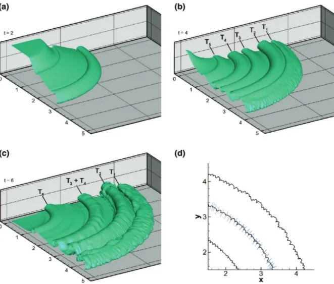
The start of the simulation is initiated by “lifting” the cylindrical gate. The particle-laden solution is heavy and begins to collapse and spread out radially, intruding into the ambient fluid with a slug-like ground hugging motion. InFig. 3, we present iso-surfaces of concen-tration from the large Re number simulation of 10,000 to help visual-ize the three-dimensional temporal and spatial structures of the cur-rent as well as bottom iso-contours of concentration showing the lobe and cleft structures at the front. Shortly after release (t = 2), the front is nearly two-dimensional and the “head” of the current may be rec-ognized by a rolled up vortex tube at the front. At later times (t = 4 and t = 6), a pattern of rolled up vortices can be identified. Because of their unequal propagation speeds, some of the relatively faster vor-tex tubes will catch up with slower tubes ahead and merge to form bigger rolled up vortices (seeFig. 3at t = 4 and t = 6) Furthermore, as the current starts to decelerate, (and because of the no-slip bound-ary condition at the bottom surface) lobe and cleft structures[21, 15] begin to emerge rendering the once smooth front more complex and

three-dimensional. The speed of the current continuously develops along its circumference, and as a result, the lobe and cleft structures evolve by merging and splitting along the front. InFig. 3d, the cur-rent’s front at three time instances is identified by the bottom iso-contour of

φ

=0.05. There we observe the lobes and clefts to grow in size from t = 2 to t = 4,and then maintain roughly the same size at

t = 6. At t = 4, we may roughly estimate the number of these lobes

and clefts where we observe the presence of 23 lobes (or clefts) in the chosen portion of the domain (x ≥ 1.5, y ≥ 1.5) This translates to approximately 200 lobes (or clefts) along the entire front. The thin dashed lines inFig. 3d mark the locations of the clefts. Computing the mean front perimeter at t = 4, one may estimate the character-istic wavelength of the lobes and clefts to be roughly 1/10 the ini-tial height of the current. This is in reasonable agreement with the characteristic size of lobes and clefts predicted by the linear stability analysis of Hartel et al.[15]in the case of a planar gravity current, for which the predicted wavelength is in the range 0.03–0.1 for Grashoff numbers between 5 × 106_{and 5 × 10}8_{(the Grashoff number of the}

present simulation is 107_).

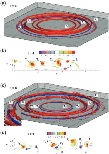
The primary vortical structures identified in Fig. 3(T1−T4) are

the Kelvin-Helmholtz vortices generated at the current–ambient interface. These vortices exhibit a counter-clockwise rotation (in this paper, the direction of rotation of a vortex tube (clockwise or counter-clockwise) is taken to be that seen on the x-z plane viewed in the positive y-direction) and are advected radially outwards by the current. These energetic vortices locally accelerate the flow in the near wall region, and because of the no-slip boundary condition, help to initiate clockwise-rotating vortices at the bottom surface. The flow, in the near wall region, accelerates as it passes between the counter-clockwise rotating vortex and the bottom wall, and its dynamic pressure locally decreases. The flow then decelerates, as it passes be-yond the radial location of the toroidal vortex tube, and is subjected to an adverse pressure gradient, which results in flow separation and the initiation of a clockwise-rotating bottom vortex(B1−B3) in

Fig. 4d. These bottom vortices are concealed in the iso-surface plots, but may be readily visualized through iso-surface plots of the swirling strength

λ

cishown inFig. 4. The swirling strength is a good

indicator of regions of intense vortex structures[28,7]. It is defined as the absolute value of the imaginary portion of the complex eigen-value of the velocity gradient tensor. At t = 4, the domain consists of four well-defined primary vortex tubes (T1−4) that span the head and

body of the current. In addition to these tubes, the bottom vortex ring

B1starts to form just behind the head, where a set of closely packed,

inclined hairpin vortices emerge from the surface denoting the elevated head of the current. At t = 6, two additional bottom vortex tubes have appeared (B2and B3) and the overall vortical structures

have become more complex. In the body of the current, inclined hairpin vortices have formed around the vortex tube B2(see inset).

The typical dimensional turnover time

τ

=T/

(λ

ci

)

maxof the large

scale vortical structures may be inferred from the maximum value of

λ

ci(located at the center of each vortex) for each of these toroidal

vortices. Moreover, by comparing the ratio of the dimensional Stokes time of the particles

(τ

s=us/g

)

to the dimensional typical turnover time

τ

of the large scale vortical structures, we may verify, and assess (a posteriori) the validity of our numerical model, specifically that the particle velocity updefined in (3) may be directly obtained as the

sum of the fluid velocity u and the settling velocity us. The maximum

value of the ratio of

ξ

=

_τ

_s/

τ

was computed as a function of time and was always found to be less than 1%. This confirms that the present model, (i.e.Eq. 3), is appropriate in the present case.

3.2. One-dimensional time evolution

InFig. 5, we plot the temporal evolution of the mean height ¯h and areal deposit ¯D of the current along the radial direction. These

Fig. 3. (a)->(c) Iso-surfaces of concentration in first quadrant (x ≥ 0, y ≥ 0) of the computational domain for Re = 10000 . The structure of the current exhibits multiple

rolled-vortices with the lobe and cleft instability pattern identifiable at later times(t = 6). An isovalue ofφ=0.25 is employed for all cases. (d) Iso-contours ofφ=0.05 at the bottom wall for t = 2, 4, 6 .Multiple lobe and cleft structures may be identified. Blue lines are added on the contour at t = 4 to show the characteristic size of these structures.

directions for the concentration field to calculate ¯h, and integrating in time the tangentially-averaged bottom concentration section (multiplied by the settling velocity) to obtain ¯D

¯h

(

r, t

)

= 1 2

π

Z H 0 Z 2π 0

φ(

r,

θ

,z, t

)

d

θ

dz ¯ D

(

r, t

)

= 1 2

π

Zt 0 Z2π 0

φ(

r,

θ

,0, t

)

usd

θ

dt (7)

Initially, the areal deposition along the lock length (0 ≤ r ≤ R0)

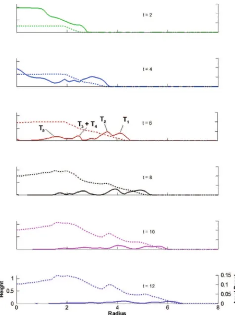
in-creases linearly with time up to the point where all the fluid inside the lock has been set in motion (t ≈ 6). The current is shown to attain the typical slug like shape with a relatively thick head and a slen-der body around t = 4. At t = 10, the areal deposition profile begins to converge towards its final form with two local maxima becoming identifiable with the largest of the two developing at close proximity to the gate at a radial distance of r = 2, and the smaller of the two ap-pearing farther downstream around r = 3.5. As seen fromFig. 6, the effect of sedimentation on the spreading rate of the current is not per-ceived until enough particles have settled out. This occurs sometime between t = 10 and t = 16, where the particle-laden current front be-gins to deviate from the saline current. During that time frame, the current has lost over 45 percent of its total particles (seeFig. 7).

3.3. Front location

The front position of the current is shown inFig. 6. Because of the axisymmetric nature of spreading, the concentration field is first averaged in the azimuthal direction. The position of the front (rN) is

then taken as the location where the vertically averaged concentra-tion (the current’s thickness) drops to a value of 0.01. Our numerical domain was chosen to match the physical setting of experiments re-ported by Bonnecaze et al.[3], and their findings are plotted alongside our simulation data inFig. 6. Our results for the larger and smaller Re number simulations are in good agreement with the experiments and the Shallow Water equations-based theoretical model. The larger Re number case of 10,000, which is closer to the Re of the experiments of 17,000, provides however, slightly better agreement with the exper-iments and SW model. In addition to the particle-laden currents, we also show the front location for a saline current experiment carried out by Bonnecaze et al.[3]. The saline current experiment serves as a benchmark to identify the time beyond which sedimentation effects influence the front velocity of the particle-laden current.

The aforementioned experiments were carried out in a radial sec-tor tank with monodisperse 37

µ

m silicon carbide particles resulting in a non-dimensional settling velocity of 1.3 × 10−2_{.This is precisely}

the non-dimensional settling velocity used in the present simula-tions. The initial reduced gravitational acceleration for the particle-laden and saline currents were 11 cm s−2_{and 42 cm s}−2_{, respectively.}

T2 T4 T3 T1 B1 r z 1 2 3 4 0 0.2 0.4 -6 -4.5 -3 -1.5 1.5 3 4.5 6 t = 4 T5 r z 1 2 3 4 0 0.2 0.4 -8 -6 -4 -2 2 4 6 8 B3 T3+ T4 B1 T2 t = 6 B2 T1

(a)

(b)

(c)

(d)

Fig. 4. (a) and (c) iso-surfaces ofλci(multiplied by the sign of the azimuthal vorticity

|ωθ|/ωθ) for Re = 10000 with isovalues of 6 and 8 for t = 4, and t = 6, respectively. A close-up view at t = 6 shows a set of inclined hairpin vortical structures that have formed around the bottom clockwise rotating vortex B2in the body of the current. The blue (resp. red) color indicates clockwise (resp. counter-clockwise) rotation. (b) and (d) contours ofλci(multiplied by the sign of the azimuthal vorticity |ωθ|/ωθ) in the vertical y = 0 plane for t = 4, and t = 6, respectively. (For interpretation of the references to

color in this figure legend, the reader is referred to the web version of this article).

Despite the difference in the reduced gravitational acceleration, the non-dimensional front positions of these currents perfectly match until enough particles have settled out and the two curves begin to diverge from one another.

3.4. Deposition

Of fundamental importance in particle-laden gravity currents is the deposition pattern of sediments. The settling of particles leads to a continuous decrease in the density of the current leading to a decay in the driving force, and eventually causing the current to arrive at a standstill when all the particles have settled out. The total deposited mass (normalized by the initial mass in the domain), M, is shown in Fig. 7for the Re = 3450 and Re = 10000 cases. Here, M is computed as M

(

t

)

= RLy 0 RLx 0 Rt 0

φ(

x, y, 0, t

)

usdt dx dy RLy 0 RLx 0 RH 0

φ(

x, y, z, 0

)

dz dx dy . (8)

Both curves are in good agreement up to t ≈ 10 at which point the total mass deposited from the Re = 10000 case becomes larger than that corresponding to the Re = 3450 case. This is somewhat counter-intuitive as one would expect enhancement of turbulence to better

mix (destratify the concentration profile) and thus hinder the depo-sition process. However, there are other factors that could affect the deposition rate in the simulations. The horizontal extent of the cur-rent could be such a factor. The wider the surface the curcur-rent cov-ers, the larger the area overwhich the current can deposit particles. FromFig. 6, we observe the current for the Re = 10000 case to ad-vance faster and cover more distance than for the Re = 3450 case. In particular at t = 30, the run out distance for the Re = 10000 (resp.

Re = 3450) case is 9.1 (resp. 8.6). This results in an area increase of

12%, and provides a possible explanation to the enhanced deposi-tion for the larger Re case. In the inset ofFig. 7, we show the total deposited mass M further normalized by the horizontal area of the current,

π

r2

N, and then multiplied by 1000. Here we observe that the

lower Re case beyond t ≈ 8 to deposit more sediments per unit area of the current. As mentioned earlier, the lower the Reynolds number, the more stratified the vertical concentration profile, and the larger the deposit per unit area of the current.

Fig. 8illustrates the temporal evolution of the rate of deposition of suspended particles defined as

˙ m

(

t

)

= ZLy 0 Z Lx 0

φ(

x, y, 0, t

)

usdx dy (9)

We observe a rise in the sedimentation rate from the time of release up to t = 8, beyond which the particles continue to settle but at a continuously diminishing rate. Immediately after release, the current begins to deposit particles over a circular surface of ra-dius R0. However, as the current starts to spread radially outward,

its surface area increases with the bottom concentration remaining at a relatively high level leading to a rise in the sedimentation rate as observed in Fig. 8(0 < t < 8). At a certain instant however (t ≈8), the bottom concentration has become dilute enough, that the deposition rate begins to decline despite its continuously increas-ing front position. This behavior of rise and decay in the sedimen-tation rate has been also observed for planar particle-driven gravity currents[18].

The local instantaneous deposition rate is strongly affected by the large-scale vortex tubes shown inFig. 4. These tubes create local min-ima in the instantaneous bottom concentration profile (and hence the instantaneous deposition rate) by transporting low concentration fluid (particle-laden current mixed with the ambient) towards the bottom wall. Consider for instance the 2-dimensional concentration profile on the bottom wall at t = 6 as shown inFig. 9. We may readily identify a local minimum at r ≈ 2.5, where the bottom concentration drops by about 14%. The position of this minimum corresponds to the radial location of the vortex tube labeled T3+T4. Except for the

afore-mentioned drop in the bottom concentration at r ≈ 2.5, the current appears to deposit its sediments uniformly in the domain 1 < r < 3.5. At r ≈ 4 however, the three-dimensionality of the flow is strong due to the effect of the lobe and cleft instability at the front as well as the inclined hairpin vortices that emerge from the bottom wall around the front of the current as seen inFig. 4.

For the sake of comparison with experiments, we plot inFig. 10 the areal deposition from both simulations and compare them with Bonnecaze et al.[3]experimental and theoretical final deposition lay-out. The areal density of deposit of the simulations is taken at t = 30, at which point over 95% (resp. 91%) of particles have settled for the

Re = 10000 (resp. Re = 3450) case.

The simulation curves are scaled so that the area under the curve is equivalent to that of the experimental results. The simulations as well as the theoretical model indicate that the current’s density of deposit increases as we move away from the center and reaches a maximum value close to

(

r = 2

)

.This is in contrast with the exper-iments where the density of deposit decreases monotonically as we move radially outwards. Differences between simulation and exper-iments are most distinct in the region around the lock. However, for the experiments, the region behind the gate is subject to disturbances

Fig. 5. Height (solid line) and areal deposit (dashed line) as a function of radius for different times with Re = 10000. The four peaks in the height profile at t = 6 correspond to the

Kelvin–Helmholtz vortices shown inFig. 3. The Kelvin–Helmholtz vortices at t = 4 are not as readily identifiable, perhaps because of the relatively smaller radial variations in the density profile.

Fig. 6. Evolution of the front as a function of time. The solid and dash-dotted lines

are from the present simulation. The circular and triangular symbols are from Bon-necaze et al.[3]experiments for particle-laden currents with 37µm-diameter silicon carbide particles with an initial reduced gravity of g′

0=11 cm s−2-, and a saline cur-rent with g′

0=42 cm s−2, respectively. The dashed line is the solution of a theoretical model based on the Shallow Water equations from Bonnecaze et al.[3].

from initial stirring in addition to the early sedimentation that initi-ates before the removal of the gate. The DNS results inFig. 10, also reveal a second peak in the amount of deposition at a downstream

Fig. 7. Total mass of settled particles as a function of time forRe = 3450 and Re =

10000. Results are normalized with the initial mass of suspended particles. (Inset) Same as main figure, but results are further normalized by the horizontal area of the current and multiplied by 1000.

location from the gate. It should be noted however that the ampli-tude of these peaks is observed to decrease with increasing Reynolds number. The presence of multiple spikes have also been observed in planar simulations of particle-laden currents[18].

Fig. 8. Deposition rate versus time at the bottom wall of the domain for Re = 10000.

The sedimentation rate increases from the time of release, attains a maximum value around t = 8, then monotonically diminishes up to the end of the simulation.

Fig. 9. Contours of concentration at the bottom wall for Re = 10000 in one quadrant

of the computational domain at t = 6. The large scale vortex tubes transport low con-centration fluid (particle-laden fluid mixed with the ambient) from the top of the cur-rent towards the bottom wall resulting in a local minimum around the radial distance

r = 2.5.

Fig. 10. Final areal density of deposit from simulation, experiment, and theoretical

model. The experiments and theoretical model results are extracted from Bonnecaze et al.[3].

3.5. Wall shear-stress and near-wall dynamics

Exploring the near-wall dynamics of a particulate gravity current is necessary for understanding erosion and resuspension of particles. The wall-shear stress is often used in theoretical models to predict the possibility of sediment entrainment over loose beds[25,27,19]. The dimensional wall-shear stress in the radial direction is defined as

τ

w=

µ

∂

u∗ R

∂

z∗

¯

¯

¯

¯

_z∗₌₀ (10) where,

µ

represents the dynamic viscosity of the current, u∗

R is the

dimensional horizontal component of velocity in the radial direction,

Fig. 11. Contours of the radial bottom shear stress for Re = 10000 in one quadrant of

the computational domain at t = 6. The wall shear stress is strongly affected by the clockwise-rotating bottom vortex tubes shown inFig. 4. Here, the wall-shear stress is multiplied by Re/(ρ∗

c0U2), whereρ

∗

c0is the dimensional initial density of the current.

Fig. 12. In-plane velocity field in the vertical, y = 0, plane at t = 4 and t = 6 for Re =

10000 case. The current layout is visualized by a concentration contour ofφ=0.05. The top (resp. bottom) vortices rotate with a counter-clockwise (resp. clockwise) di-rection.

and z∗_{=z × H is the dimensional vertical coordinate (z}∗₌₀

signify-ing the location of the bottom plane).

These bed-shear stresses are closely related to the large scale clockwise rotating vortex tubes discussed in Section 3.1. A two-dimensional contour plot inFig. 11of the wall shear-stress at t = 6 reveals three local minima with a local region of reversal in flow di-rection (negative wall shear-stress). These local minima correspond to the clockwise rotating vortex tubes sweeping the bottom wall (B1,

B2, and B3). The vortex tubes B1and B3 are relatively smooth with

small variations along the radial direction. Their axisymmetric struc-ture is translated into a smooth shell-like outline in the wall shear-stress contours ofFig. 11. On the other hand, the hairpin and other small-scale vortical structures forming around B2(seeFig. 4) is the

reason behind the wavelike pattern at r ≈ 2.8 inFig. 11. The local minima in the bottom shear-stress profile ofFig. 11are a result of flow reversal due to the aforementioned clockwise vortex tubes ro-tating at close proximity to the bottom wall. The direction of these vortices and their position with respect to the current is presented in Fig. 12. Here, a vertical two-dimensional section of the domain (y = 0 plane) shows the in-plane velocity field along with the position of the current visualized by a contour of

φ

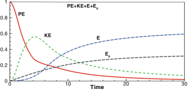
=0.05. The current is observed to take a slug-like shape constituting of a head and a body, where the head extends from the front of the current (r ≈ 4.5) until the location

Time 0 10 20 30 0 0.2 0.4 0.6 0.8 1 Ep PE+KE+E+Ep KE _E PE

Fig. 13. Temporal evolution of the potential energy (PE), kinetic energy (KE), and

dis-sipation (E and Ep), defined in (11) and (16), respectively, of the Re = 10000 turbidity

current. The sum of all four terms is shown as the thin black line.

of the top vortex T1, (r ≈ 4). The body is seen to have multiple

undu-lations mostly caused by the top counter-clockwise rotating vortices.

3.6. Energy budget

The potential to kinetic energy transformation is of fundamental interest in the study of gravity currents. In the present setup, the total potential (PE) and kinetic (KE) energies are defined as

PE

(

t

)

= ZH 0 Z Ly 0 ZLx 0

φ

z dxdydz KE

(

t

)

= 1 2 ZH 0 Z Ly 0 ZLx 0 u2dxdydz. (11)

Initially, all the energy in the domain is in the form of potential en-ergy, however as the current begins to spread, part of this potential energy is used to set the flow in motion, while part is lost to viscous dissipation. There are two types of dissipation for particle-laden cur-rents. The first, denoted here as

σ

, is a result of the gradient of the meso-scale velocity field, it is defined as

σ (

t

)

= 2 Re ZH 0 ZLy 0 Z Lx 0

ε

·

ε

dxdydz, ₍₁₂₎

where ɛ is the strain-rate tensor of the computed meso-scale veloc-ity field. The second type of dissipation is at the micro-scale and is caused by the Stokes flow around the individual particles[10]. Even though our numerical model does not resolve the flow around the in-dividual particles, the latter dissipation may be computed from the local concentration field, viz

σ

p

(

t

)

= − ZH 0 ZLy 0 ZLx 0

µ

1 ScRez

∇

2

_φ

_{+z u} s

∂φ

∂

z

¶

dxdydz. (13)

The global energy budget, which is derived from the momentum and transportEquations (2)and (4), respectively, may be expressed as

D

Dt

(

PE + KE

)

+

σ

+

σ

p=0, (14)

Integrating (14) with respect to time, we obtain

PE + KE + E + Ep=PE0, (15) where E = Z t 0

σ (η)

d

η

, Ep= Zt 0

σ

p

(η)

d

η

, (16)

and PE0=PE

(

t = 0

)

is the total initial potential energy in the domain.

Fig. 13shows the temporal evolution of the four terms on the left hand side of (15) normalized by PE0. During the early stages of the

release (up to t = 4), there is a fast conversion of potential to kinetic energy, as the current loses around 70% of its initial potential energy.

This fast decline in the available potential energy is accompanied by a rapid increase in kinetic energy. Beyond that time, the potential en-ergy in the system continues to drop due to the finite nature of the release (no external source of energy), whereas the kinetic energy is observed to reach a maximum value (KE ≈ 0.56PE0) around t = 5

be-fore starting to decay as a result of viscous dissipation, in the present case of cylindrical release for which Re = 10000 and up=0.013. The

dissipation is mostly dominated by Epin the early stages of the flow

(up tot ≈ 5), however as more particles settle out towards the bot-tom wall, the macroscopic dissipation term E becomes the dominant dissipation term being almost twice as large as that due to sedimen-tation at larger times, say t > 20. Note that in the case of a planar release with Re = 2236 and up=0.02, Necker et al.[18]found a

simi-lar evolution of the kinetic energy and dissipation, as in their case the maximum value of KE was 0.52PE0at t = 3 and E = 1.5Epfor t > 20,

approximately. The lower value of E relative to Epin their case may

be attributed to the larger value of the settling velocity (up=0.02 vs 0.013 in our case) which is likely to increase the contribution of dis-sipation due to sedimentation.

4. Conclusions

We present direct numerical simulation results for a cylindrical, finite-release, particle-laden gravity current. At early times (t < 6), the current shows a train of Kelvin–Helmholtz counter-clockwise ro-tating rolled up tubes that are generated along the current–ambient interface. Below these vortex tubes, a set of clockwise-rotating eddies initiate from the bottom wall. These large scale vortical structures are difficult to visualize and study experimentally and are unattainable using depth-averaged, two-dimensional theoretical models. They are nonetheless very important for studying the erosion, deposition, and resuspension dynamics of particle-laden currents. These vortex tubes may locally modify the bed shear stress and hence could play an important role in particle entrainment and erosion off the bottom wall. Furthermore, by transporting low particle concentration fluid from the surface of the current towards the bottom wall, they locally change the bottom concentration and hence modify the deposition pattern as well. Our simulations compare favorably with previous ex-periments[3]in terms of the temporal evolution of the front as well as the final deposition pattern.

Acknowledgments

This study was supported by the Chateaubriand Fellowship pro-vided by the French Embassy in the USA as well as the National Sci-ence Foundation Partnership for International Research and Educa-tion (PIRE) grant (NSF OISE-0968313). The two anonymous reviewers are thanked for their detailed and insightful comments which greatly improved the quality of the paper.

References

[1] Blanchette F, Strauss M, Meiburg E, Kneller B, Glinsky M. High-resolution numer-ical simulations of resuspending gravity currents: condition for self-sustainment. J Geophys Res 2005;110:c12022.

[2] Bonnecaze R, Huppert H, Lister J. Particle-driven gravity currents. J Fluid Mech 1993;250:339–69.

[3] Bonnecaze R, Hallworth M, Huppert H, Lister J. Axisymmetric particle-driven gravity currents. J Fluid Mech 1995;294:93–122.

[4] Cantero M, Lee JR, Balachandar S, Garcia M. On the front velocity of gravity cur-rents. J Fluid Mech 2007;586:1–39.

[5] Cantero M, Balachandar S, Garcia M. High-resolution simulations of cylindrical density currents. J Fluid Mech 2007;590:437–69.

[6] Cantero M, Balachandar S, García M. An Eulerian–Eulerian model for gravity cur-rents driven by inertial particles. Int J Multiphase Flow 2008;34:484–501.

[7] Chakraborty P, Balachandar S, Adrian R. On the relationships between local vortex identification schemes. J Fluid Mech 2005;535:189–214.

[8] Choi S-U, Garcia M. Modeling of one-dimensional turbidity currents with a dissipative-Galerkin finite element method. J Hydra Res 1995;33(5):623–48.

[9] Dade W, Huppert H. A box model for non-entraining suspension-driven gravity surges on horizontal surfaces. Sedimentology 1995;42:453–71.

[10]Espath LFR, Pinto LC, Laizet S, Silvestrini JH. Two-and three-dimensional di-rect numerical simulation of particle-laden gravity currents. Comput Geosci 2014;63:9–16.

[11]Garcia M, Parker G. Experiments on the entrainment of sediment into suspension by a dense bottom current. J Geophys Res 1993;98(C3):4793–807.

[12]Gladstone C, Phillips JC, Sparks RSJ. Experiments on bidisperse, constant-volume gravity currents: propagation and sediment deposition. Sedimentology 1998;45:833–44.

[13]Gladstone C, Woods A. On the application of box models to particle-driven gravity currents. J Fluid Mech 2000;416:187–95.

[14]Hallworth M, Huppert H. Abrupt transitions in high-concentration, particle-driven gravity currents. Phys Fluids 1998;10:1083.

[15]Härtel C, Carlsson F, Thunblom M. Analysis and direct numerical simulation of the flow at a gravity-current head. Part 2. The lobe-and-cleft instability.. J Fluid Mech 2000;418:213–29.

[16]Hogg A, Hallworth M, Huppert H. On gravity currents driven by constant fluxes of saline and particle-laden fluid in the presence of a uniform flow. J Fluid Mech 2005;539:349–85.

[17]Lowe DR. Sediment gravity flows: II Depositional models with special reference to the deposits of high-density turbidity currents. J Sed Res 1982;52.

[18]Necker F, H¨artel C, Kleiser L, Meiburg E. High-resolution simulations of particle-driven gravity currents. Intl J Multiphase Flow 2002;28:279–300.

[19] Parker G, Fukushima Y, Pantin HM. Self accelerating turbidity currents. J Fluid Mech 1986;171:145–81.

[20]Shringarpure M, Cantero M, Balachandar S. Dynamics of complete turbulence suppression in turbidity currents driven by monodisperse suspensions of sedi-ment. J Fluid Mech 2012;712:384–417.

[21]Simpson JE. Effects of the lower boundary on the head of a gravity current. J Fluid Mech 1972;53:759–68.

[22] Simpson JE. Gravity currents in the laboratory, atmosphere, and ocean. Ann Rev Fluid Mech 1982;14:213–34.

[23] Sequeiros O, Naruse H, Endo N, Garcia M, Parker G. Experimental study on self-accelerating turbidity currents. J Geophys Res 2009;114:C05025.

[24]Ungarish M, Huppert H. The effects of rotation on axisymmetric gravity currents. J Fluid Mech 1998;362:17–51.

[25] Yalin MS, Karahan E. Inception of sediment transport. J Hydraul Div 1979;105(11):1433–43.

[26] Ziskind G, Fichman M, Gutfinger C. Resuspension of particulates from surfaces to turbulent flows – review and analysis. J Aerosol Sci 1995;26:613–44.

[27]Zeng J, Lowe DR. Numerical simulation of turbidity current flow and sedimenta-tion: I. Theory.. Sedimentology 1997;44(1):67–84.

[28] Zhou J, Adrian R, Balachandar S, Kendall T. Mechanics for generating coherent packets of hairpin vortices. J Fluid Mech 1999;387:353–96.