OATAO is an open access repository that collects the work of Toulouse
researchers and makes it freely available over the web where possible
Any correspondence concerning this service should be sent
to the repository administrator:
[email protected]
This is an author’s version published in:
https://oatao.univ-toulouse.fr/26712
To cite this version:
Boutsikakis, Athanasios and Fede, Pascal and Pedrono,
Annaig and Simonin, Olivier Numerical simulations of short
‑
and long
‑
range interaction forces in turbulent particle
‑
laden
gas flows. (2020) Flow, Turbulence and Combustion. 1-27.
ISSN 1386-6184
Official URL:
https://doi.org/10.1007/s10494-020-00115-3
Numerical Simulations of Short‑ and Long‑Range Interaction
Forces in Turbulent Particle‑Laden Gas Flows
Athanasios Boutsikakis1 · Pascal Fede1 · Annaïg Pedrono1 · Olivier Simonin1
Abstract
The main objective of this work is to study the effects of distance-dependent interactions in turbulent gas-particle flows using an Euler–Lagrange simulation approach. The turbu-lent gas flow is accounted for via Direct Numerical Simulation to the Kolmogorov scale using a spectral method to solve the Navier–Stokes equations in a cubic computational domain with tri-periodic boundary conditions. This flow simulation is coupled (one-way) with a Lagrangian particle phase solver that performs particle trajectory tracking. Electro-static forces can be calculated using two different approaches. Firstly, the direct method consists of a sum of all inter-particle interactions for all the particles of the computational domain and their periodic images. However, this purely Lagrangian approach is computa-tionally costly for a large number of particles, therefore another approximative approach is considered. According to it, one can estimate the short-range interactions via a sum of inter-particle interactions within a cut-off distance and the long-range ones via a sum of particle interactions with clusters of particles that, from a distance greater than the cut-off, are “seen” as one pseudo-particle. This method is then adjusted in order to accommodate periodic boundary conditions, which are not trivial in the case of electrostatic interactions as periodicity entails an infinite number of periodic domain images that has to be truncated to a finite number. Simulations are then performed by varying the properties of the parti-cles in terms of diameter, density (Stokes number) and charge (electrostatic Stokes num-ber). Finally, a statistical analysis is performed in order to investigate how the dynamics of the turbulent gas-particle flow are affected by distance-dependent particle–particle interac-tions, namely electrostatic forces.
1 Introduction
Particulate flows are found in many practical applications from geophysical flows (pyro-clastic flow, s ediments t ransport, v olcano a shes d ispersion, . ..) t o i ndustrial a pplica-tions (pneumatic conveying, olefin polymerization, Fluid Catalytic Cracking of oil, silo discharge, ...). In these systems the inter-particle collisions or the particle-wall bounc-ing may lead the particles to accumulate electric charges which modify the dynamic behavior of the particles. As for example in fluidized beds (Rokkam et al. 2010; Kole-hmainen et al. 2016), charges may lead the particles to form agglomerates (Ciborowski and Wlodarski 1962) that can change the fluidization regime or to adhere on the walls (Hendrickson 2006). In case of pneumatic conveying (Joseph and Klinzing 1983) or solid entrainment (Baron et al. 1987), charges may also alter granular flow dynamics. Effects of charges on particle dynamics have also been identified in geophysical flows especially for dust emission (Esposito et al. 2016) and for the saltating motion of grains (Schmidt et al. 1998; Zheng et al. 2006). Finally, electrostatic forces may be important in colloids, particularly regarding deposition (Li and Ahmadi 1993).
The present study is dedicated to the dispersion of inertial charged particles in tur-bulent flows. Several literature studies have been dedicated to charged particles trans-ported by homogeneous isotropic turbulence (Lu et al. 2010; Lu and Shaw 2015; Karnik and Shrimpton 2012; Yao and Capecelatro 2018; Di Renzo and Urzay 2018) or by tur-bulent channel flow (Rambaud et al. 2002). These studies essentially focus on the modi-fication of preferential concentration in the case of charged particles. Indeed, when solid non-charged particles are transported by a turbulent flow field, according to their iner-tia, they may accumulate in low-vorticity regions of the turbulence (Squires and Eaton 1991; Fessler et al. 1994). Such a mechanism leads to large local concentrations of par-ticles that may modify the collision rate (Sundaram and Collins 1997; Reade and Col-lins 2000) or the coalescence rate if droplets are considered instead of solid particles (Wunsch et al. 2010). Furthermore, external forces may modify preferential concen-tration, as for example, Fede and Simonin (2010) showed that inter-particle collisions enhance preferential concentration. In addition, Dejoan and Monchaux (2013) investi-gated experimentally the effect of gravity on preferential concentration. Lu et al. (2010), Lu and Shaw (2015), Karnik and Shrimpton (2012), Yao and Capecelatro (2018) show that preferential concentration decreases when charges increase. However, they do not investigate how particle dispersion, in terms of agitation, is modified by e lectrostatic interactions. Basically, particles transported by stationary homogeneous isotropic turbu-lence follow the Tchen–Hinze theory (Hinze 1972) that entails that the particle kinetic energy is directly linked to the fluid agitation (see for example Zaichik et al. 2003; Fede and Simonin 2006) via fluid–particle v elocity c ovariance. H owever, L aviéville e t a l. (1997) and later Fede et al. (2015) showed that when inter-particle collisions occur, par-ticle agitation decreases even for elastic collisions. The way that electrostatic forces act on the particles is similar to collisions via the mechanism of Coulomb collisions typi-cally found in cold plasma (Callen 2003).
In the present paper, DNS of stationary homogeneous isotropic turbulence are per-formed and coupled with Lagrangian tracking of the particles. Details of the physi-cal problem are given in Sect. 2 and the numerical methods deployed are described in Sect. 3 with focus on the algorithm that accounts for electrostatic forces. The main material properties and statistics of the turbulence and particles are both given in Sect. 4. In this section, the case without charge is briefly analyzed. The main part of the
paper is Sect. 5 where the effect of charges on the dispersion of inertial particles is ana-lyzed. Conclusions are drawn in the last section of the paper.
2 Governing Equations for Charged Particles Transported
by a Turbulent Fluid Flow
The studied configuration is a stationary homogeneous isotropic turbulent gas flow car-rying mono-disperse inertial particles. The incompressible Navier–Stokes equations are solved by using a pseudo-spectral method. Periodic boundary conditions are applied on fluid and particle phase. Statistically steady flow is achieved by using the forcing scheme proposed by Eswaran and Pope (1988). The solid mass loading is sufficiently low for neglecting the turbulence modulation by the presence of particles.
The particles are considered as mono-disperse, with diameter dp , and inertial, with
den-sity 𝜌p≫ 𝜌f . According to Maxey and Riley (1983) and Gatignol (1983), for the case of a
large particle-to-fluid density ratio and for a particle diameter that is smaller than the Kol-mogorov length scale, the force acting on the particles is only the drag force 𝐅𝐝 . In
addi-tion, if the particles are charged, then electrostatic force 𝐅e may also be significant. Particle
motion is governed by
where 𝐱p is the particle position and 𝐮p the particle velocity. In Eq. (2), the fluid–particle
drag force is calculated by
where 𝜏p is the particle relaxation time given by Schiller and Naumann (1935)
with 𝜈f the kinematic fluid viscosity, and Rep= dp‖𝐮p− 𝐮f@p‖∕𝜈f the particle Reynolds
number. In Eq. (3), 𝐮f@p is the undisturbed fluid velocity at the particle position. The
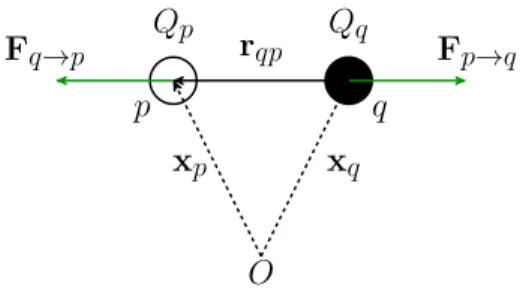
parti-cle positions and velocities are time-advanced by a second order Adams-Bashforth scheme. Coulomb’s law allows to calculate the electrostatic force 𝐅q→p acting on p due to q as
following
where 𝜆 is Coulomb’s constant (with 𝜆 = 1∕(4𝜋𝜖0
)
where 𝜖0 is the vacuum permittivity),
Qp is the electric charge of particle p and 𝐫qp= 𝐱p− 𝐱q is the distance vector between parti-cles p and q pointing to p as depicted in Fig. 1.
(1) d𝐱p dt =𝐮p (2) mp d𝐮p dt =𝐅e+ 𝐅d (3) 𝐅d= −𝐮p− 𝐮f@p 𝜏p mp (4) 𝜏p= 𝜌pdp 2 18𝜌f𝜈f 1 1+ 0.15Rep0.687 (5) 𝐅q→p= 𝜆QqQp ‖𝐫qp‖3 𝐫qp
In a system of Np charged particles, each particle p interacts with all Np− 1 particles in
the computational domain, thus the total electrostatic force exerted on p is
Next section is dedicated to the numerical methods for computing electrostatic force 𝐅e.
3 Numerical Methods for the Computation of Electrostatic Forces
3.1 Direct Dipole Summation
This method consists in calculating the total electrostatic force on a particle p by directly summing all the Np− 1 terms that correspond to the electrostatic interactions of the
par-ticle with all parpar-ticles but itself as seen by Eq. (6). However, one could use Newton’s 3rd law for such a dipole that gives 𝐅p→q= −𝐅q→p in order to perform one operation per dipole
thus divide the computational cost by two resulting in Np
(
Np− 1
)
∕2 ∼ Np2 operations
which is forbiddingly expensive.
3.1.1 Quasi‑periodic Boundary Conditions
Periodic boundary conditions for the particle phase correspond to an infinite domain. Therefore, to compute the electrostatic forces it is necessary to take into account the con-tributions of all particles, including those not really represented/computed in the computa-tional domain.
Let a cubic computational computational domain 𝛺 of length L (see Fig. 2). Conse-quently, consider a super-domain (due to periodic BCs) of (finite) length (2Nper+ 1)L ,
where Nper is the number of domain images per direction. If d is the number of (periodic)
physical dimensions, then the number of periodic domain images including the original domain is Nim=
(
2Nper+ 1)d . In theory, periodic boundary conditions are exactly repre-sented for Nper→ ∞ , however in practice Nper will be considered finite based on a
con-vergence criterion [see Eq. (8)] which entails an approximation error, thus these BCs are considered as quasi-periodic.
Therefore, each particle in 𝛺 has Nim− 1 periodic images, and the electrostatic force
act-ing on a particle p due to a particle q is the sum of all Nim interactions due to q and its images.
(6) 𝐅e= Np ∑ q= 1 q≠ p 𝐅q→p.
Fig. 1 Notations in electrostatic interaction of a dipole of iso-charged particles
which implies the particle electric potential energy diverges quadratically for tri-periodic boundary conditions as shown by Fig. 3.
(7) Uep= 𝜆Qp Np � q= 1 q≠ p Qq Nper � m, n, l= −Nper ‖̃𝐫qp‖ ≤ NperL 1 ‖̃𝐫qp‖ ∝ Nper2. Fig. 2 The computational
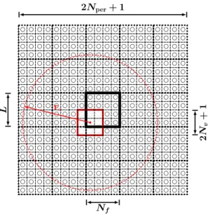
domain of interest is marked with bold contours and hatched in gray lines and its periodic images in white font. Two particles are put in the domain for simplic-ity and for each one, a spheri-cal periodic volume of radius ‖𝐫c‖ = NperL is centered at their
respective positions
Hence, in the case of tri-periodic BCs, in order to calculate the total electrostatic force exerted on p, one should perform the sum of Eq. (6) over all NpNim particles in the super-domain.
However, the computational domain (and its periodic images) is cubic, so a particle that is away from the domain center would be subjected to a force that always points outwards of the domain due to an anisotropic long-range electrostatic force distribution (see Fig. 2). In fact, this force would be proportional to the offset of the particle from the center of the computa-tional domain. As a result, all particles would accelerate towards the domain borders and due to periodicity reenter from the opposite side, where they would re-accelerate outwards, which would eventually result in an oscillation of the particles around the borders. This behavior is not physical and in order to avoid it, each particle p interacts with the particles (images) that are located within a sphere (𝐱p, 𝐫c) , where ‖𝐫c‖ = NperL , in order to ensure an isotropic
long-range electrostatic force distribution.
In practice, if the positions of Np particles in the domain 𝛺 are known, then for the
calcula-tion of 𝐅ep only Np − 1 distance vectors 𝐫qp are needed for Np − 1 particles q in 𝛺 . Then, for each particle q, the Nim distance vectors between p and the images of particle q (including
itself) can be simply calculated as a translation of the original distance vector
𝐫̃qp = 𝐫qp + mLx𝐢 + nLy𝐣 + lLz𝐤 with m, n, l = −Nper, Nper . Apparently, for m = n = l = 0 the
distance vector is the original one. As more periodic images are taken into consideration, one particle that lies in the computational domain interacts with more particles Nim ∝ Nper
3 that
As far as the total electrostatic force on a particle is concerned, the same dynamics are in place due to periodicity, however it should be noted that 𝐅e∝ 1∕‖𝐫qp‖2∝ 1∕Nper
2 . In
addition, although the number of electrostatic interactions scales with Nper
3 , the electrostatic
force converges for Nper→ ∞ due to its vectorial nature and the symmetry of periodicity.
In fact, Fig. 4 shows that electrostatic forces converge very quickly for Nper ≥ 2 , hence for
the simulations carried out in this work, the domain is replicated two times towards each direction. Theoretically, from the point of view of a particle in the computational domain, as more particle images are taken into account around it, there is a cut-off distance after which the long-range electrostatic forces that are exerted on it tend to cancel out as Nper→ ∞ . This Fig. 3 Average particle electric potential energy with respect to the number of periodic domain images. Quadratic divergence observed as Nper→ ∞
Fig. 4 Average norm of the electrostatic force with respect to the number of periodic domain images. Con-vergence is observed for Nper≥ 2
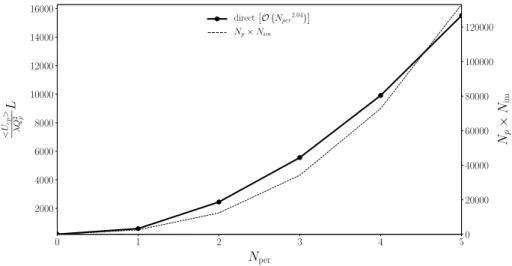
is due to an isotropic long-range force distribution around it, resulting in the convergence of its total electrostatic force to a finite value. From Eq. (6), one can deduce that
For periodic BCs, the computational cost of the direct method scales with the number of periodic images as NpNim ⏟⏟⏟ particles + images ( Np− 1)∕2 ∼ NimNp2. 3.2 Pseudo‑particle Method
Let the domain be discretized in Nf cells per dimension (see Fig. 5). For each particle p, its
neighborhood Vp of size 𝛥xv =
(
2Nv+ 1)𝛥x is defined as the ensemble of (2Nv+ 1)3 cells around it. The number of cells for which the neighborhood spans towards every direction
x, y, z (excluding the cell that contains the particle) is Nv , as illustrated by Fig. 5. Each cell
Ωk contains Nk∼ Np∕Nf3 particles and forms a pseudo-particle, which is a cluster of
parti-cles “viewed” from distance as one particle of equivalent charge Qk
eq and position 𝐱 k eq . The
concept of pseudo-particles, inspired by Barnes and Hut (1986), is defined in Eqs. (9)–(11).
with (8) 𝐅e= 𝜆Qp Np � q= 1 q≠ p Qq Nper � m, n, l= −Nper ‖̃𝐫qp‖ ≤ NperL ̂̃𝐫qp ‖̃𝐫qp‖2 ∝ Nper � m= −Nper ‖̃𝐫qp‖ ≤ NperL 𝐟𝐞𝐩 (m)= 𝐟 e. (9) Qkeq= Nk ∑ p=1 𝜒pkQp (10) 𝐱k eq= 1 Qk eq Nk ∑ p=1 𝜒pkQp𝐱p (11) 𝜒pk= { 1 particle p is in cell k 0 otherwise
Fig. 5 Computational domain of length L is discretized in Nf
cells per dimension. For each particle p, its neighborhood Vp
(red) is defined as the ensemble of (2Nv+ 1)3 cells around it. Pseudo-particles are represented as gray circles outside of Vp
Therefore, each particle interacts directly with all particles in neighborhood Vp (short-range
interaction), as well as with the pseudo-particles that are outside of Vp (long-range interaction).
The electrostatic force 𝐅k→p acting on particle p due to pseudo-particle k is calculated by
treat-ing k as another particle, meantreat-ing that in Eq. (5) Qq is replaced by Qkeq and 𝐱q by 𝐱keq.
Hence, the total electrostatic force on particle p is calculated by performing direct summa-tions in Vp and pseudo-particle summations outside of Vp.
3.2.1 Quasi‑periodic Boundary Conditions
Let the number of pseudo-particles plus their periodic images be NimNf
3 . Apparently, N v
must satisfy the inequality Nv≤
[
Nf
(
2Nper+ 1
)
− 1]∕2 in order to fit in (2Nper+ 1
)
L , as
shown by Fig. 6. As a result, the computational cost with periodic BCs becomes
Np ⎡ ⎢ ⎢ ⎢ ⎢ ⎣ � 2Nv+ 1�3Np∕N3f − 1 ⏟⏞⏞⏞⏞⏞⏞⏞⏞⏞⏞⏞⏞⏞⏟⏞⏞⏞⏞⏞⏞⏞⏞⏞⏞⏞⏞⏞⏟ inside Vp + NimNf3−�2Nv+ 1�3 ⏟⏞⏞⏞⏞⏞⏞⏞⏞⏞⏞⏞⏞⏟⏞⏞⏞⏞⏞⏞⏞⏞⏞⏞⏞⏞⏟ outside Vp ⎤ ⎥ ⎥ ⎥ ⎥ ⎦ .
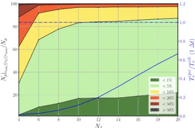
3.3 Error and Performance Analysis
An error and performance analysis of the proposed algorithm is presented in Fig. 7. As the error analysis is concerned, the direct method is considered to be of high fidelity as it allows for an exact calculation of the electrostatic forces and hence the results obtained with this method constitute a reference for simulations using other approximative methods such as the pseudo-particle method. Therefore, the relative error of total electrostatic force estimation for particle p at t = 0 is defined as 𝜖0 p= � ‖𝐅0 e��dir− 𝐅 0 e��pseudo‖ � ∕‖𝐅0 e��dir‖.
It is obvious that the latter is performing better than the former as it approximates the long-range interactions via pseudo-particles. It should also be noted that the calculated order of complexity ∼ Np1.3 is considerably better than the expected theoretical one ∼ Np1.5.
4 Numerical Simulation Setup and Flow Statistics
4.1 Numerical Schemes and Parameters
The numerical solver is fully parallelized for both the fluid and the particles. For the DNS the FFT are performed by the library P3DFFT (Pekurovsky 2012). In the present numerical (12) 𝐅e= N3 f ∑ k= 1 k∈ Vp Nk ∑ q= 1 q≠ p 𝐅q→p ⏟⏞⏞⏞⏞⏞⏞⏞⏞⏞⏞⏞⏟⏞⏞⏞⏞⏞⏞⏞⏞⏞⏞⏞⏟ short range ( 2Nv+ 1)3Np∕N3 f − 1 terms + N3 f ∑ k= 1 k∉ Vp 𝐅k→p ⏟⏞⏞⏞⏞⏞⏟⏞⏞⏞⏞⏞⏟ long range Nf3−(2Nv+ 1)3terms
f,i f ,i⟩f
rian average on the grid used for the fluid phase.
In this work, all particles are considered to bear equal positive charges. Practically, par-ticles are charged via the phenomenon of triboelectrification (Grosshans and Papalexandris 2017) which occurs when particles collide with walls and other particles. In the simulated periodic particulate flow, it is assumed that particles have had sufficient time to redistribute their charges among them via collisions. However, collisions and triboelectrification are neglected in this study because of the small solid volume fraction.
In fact, numerical simulations have been performed with Np= 10, 000 particles
corre-sponding to a solid volume fraction 𝛼p= 2.64 × 10⁻⁶ . In addition, all particles have been
considered of the same diameter so that 𝜂K∕dp= 4.56 but they differ by density. Since
par-ticle diameter is smaller than the Kolmogorov scale, parpar-ticles are numerically treated under the point-particle approximation. As such, the particle charge Qp is considered to be
con-centrated in one point (particle’s center of mass) defined as Qp= 𝜋dp2× 𝜌q , where 𝜌q the
particle surface charge density.
Fig. 6 Domain of interest 𝛺 (solid black), periodic domain images (dashed black) with
Nper= 2 and spherical periodic
volume (dashed red) with radius ‖𝐫c‖ = 2L . Neighborhood Vp
(solid red) with Nv= 1 could
span over several images of 𝛺
simulations the number of grid points for the DNS is Nx = Ny = N√z = 256 and the
turbu-lent Reynolds number, based on the integral length scale ReLf = 2∕3qf 2 L
f ∕𝜈f , is about
100. According to 𝜂K𝜅Fmax = 2.92 (where 𝜂K is the Kolmogorov length scale and 𝜅max the
highest solved wavenumber) the small turbulent scales are well resolved. As two-way cou-pling is neglected, the fluid velocity seen by the particles, 𝐮f @p , is computed by 3rd order
polynomial interpolation of the fluid velocity field. According to the previous analysis and adjusting the parameters for optimal parallelization, the electrostatic forces have been com-puted with Nf = 8 , Nv = 1 and Nper = 2.
4.2 Fluid and Particle Material Properties
The fluid material properties and main turbulence statistics are gathered in Table 1. In this table, the fluid kinetic energy is defined by qf2 = 1∕ 2⟨u
�u� where ⟨ . ⟩
Eule-(a)
(b)
Fig. 7 Error distribution (a) and performance (b) of periodic direct and pseudo-particle algorithm for
Several particle charges have been considered, all given in terms of a reference charge
Q0= 1 × 10⁻⁹C . It should be noted here, that according to Hamamoto et al. (1992) there is
a saturation limit of surface charge density for small spheres, which can be translated (via
dp ) to a corresponding limit for point-particle charges. For the configuration presented in
this work, this value can be estimated to be approximately 4 × 10⁻⁹ C, which is of the same
order of magnitude of the charges used in all simulations.
In Table 2, particle Stokes number based on the Stokes drag and the Kolmogorov time scale is given. However, as we consider non-linear drag force (see Eq. (3)), the particle relaxation time scale is introduced as 𝜏F
fp=
� ⟨1∕𝜏p⟩p
�−1
where ⟨ . ⟩p denotes a Lagrangian
average on the particle distribution.
Therefore, the Stokes number is defined as 𝜏F fp∕𝜏
t
f@p where 𝜏 t
f@p is the Lagrangian
inte-gral time scale of the fluid seen by the inertial particles. Such a timescale is defined from the Lagrangian auto-correlation function of the fluid velocity seen:
where q2
f@p= 1∕2⟨u � f@p,iu
�
f@p,i⟩p the kinetic energy of the fluid seen by the particles. The
Lagrangian fluid integral time scale is defined by
(13) Rtf@p(𝜏) = ⟨u � f@p,i(t0)u�f@p,i(t0+ 𝜏)⟩p 2q2 f@p(t0) Table 1 Properties of the fluid
and of the examined HIT Parameters Value Units Computational domain length,
Lx= Ly= Lz= L
2𝜋 m
Fluid kinematic viscosity, 𝜈f 1× 10⁻³ m2∕s
Fluid density, 𝜌f 1.0 kg∕m3
Fluid kinetic energy, qf2 3.16× 10⁻² m2∕s2
Eddy lifetime, Te= Lf∕
√ 2∕3q2
f 4.49 s
Fluid longitudinal integral length scale, Lf∕L 1.04× 10⁻¹ –
Fluid integral time scale, 𝜏t
f∕Te 6.97× 10⁻¹ –
Reynolds number, ReLf 99.39 –
Kolmogorov length scale, 𝜂K∕Lf 3.50× 10⁻² –
Kolmogorov time scale, 𝜏K∕Te 1.16× 10⁻¹ –
𝜂K𝜅 F
max 2.92 –
Table 2 Material properties of particles with
𝜏St p = 𝜌pd 2 p∕ ( 18𝜌f𝜈f ) the Stokes particle time scale
Class 𝜏St p∕𝜏K 𝜏fpF∕𝜏 t f 𝜏 F fp∕𝜏 t f@p 1 53.34 7.68 6.65 2 26.67 3.87 3.50 3 13.34 1.95 1.83 4 7.33 1.09 1.11 5 4.00 0.60 0.52 6 2.00 0.31 0.25 7 1.07 0.17 0.10 8 0.53 0.09 0.06
When motionless particles are considered, Eqs. (13) & (14) allow to compute the Eulerian time scale, 𝜏E , and for fluid elements the Lagrangian fluid integral time scale, 𝜏ft . For the
following statistical analysis we also define the particle kinetic energy, q2
p= 1∕2⟨u � p,iu
� p,i⟩p
and the fluid–particle velocity covariance as qfp=⟨u�f,iu �
p,i⟩p . Furthermore, statistical
moments have been calculated over a sufficiently long duration
Tstat= 10 × max{𝜏f@pt , 𝜏 F
fp, 𝜏el} in order to achieve statistical convergence, which is
calcu-lated as a multiple of the maximum characteristic time scales of all the physical mecha-nisms involved.
4.3 Coulomb Collisions and Characteristic Time of Electrostatic Interactions
In order to analyze the effects of the charges one should define a characteristic time scale of electrostatic interactions. This time scale is the duration of particle velocity decorrelation under the sole presence of electrostatic interactions. The mechanism of this velocity decor-relation is the Coulomb collision, which is a binary elastic collision between two charged particles interacting through their own electric field. In order to understand a Coulomb collision of two particles, we can imagine that they undergo an elastic collision with an effective Coulomb diameter dC
pq as depicted by Fig. 8. These interactions are well resolved
in the DNS carried out in this work and not modeled.The effective Coulomb diameter dC pq is
a notion typically found in cold plasma (Callen 2003) and in this case it is defined as
where 𝐰pq is the relative approach velocity of the particles defined as 𝐰pq= 𝐮p− 𝐮q and
the Lagrangian average of its norm is approximated by ⟨‖𝐰pq‖⟩p=
�
16∕𝜋 × 2∕3 × q2 p .
Additionally, mpq is the reduced mass of a pair of particles p and q calculated as
mpq= mpmq∕(mp+ mq) . If the kinetic energy of the particles is very large with respect to the electric potential energy, the deviation from the initial trajectories of the colliding parti-cles is small. Therefore, dC
pq≤ dp and particles would undergo a hard sphere collision,
however this is not treated in our simulations, as explained in Sect. 4.2. This length scale is (14) 𝜏f@pt = ∫ ∞ 0 Rt f@p(𝜏)d𝜏 . (15) dC pq= 1 𝜋⟨‖𝐰pq‖⟩p � QpQq mpq𝜖0
Fig. 8 Schematic of a Coulomb collision of two iso-charged particles and notion of Coulomb diameter. Particle diameter dp
is depicted with a solid black circle, while (fictitious) effective Coulomb diameter with a dashed black circle
also used to determine the size of the neighborhood 𝛥xv as it should be 𝜙 ≫ 1 times bigger
than the effective Coulomb diameter dC
pq . Therefore, one can deduce the number of cells Nv
in the neighborhood of short-range interactions as described in Sect. 3.
The Coulomb collision frequency is written as 𝜈c = npQc⟨‖𝐰pq‖⟩p , therefore the
charac-teristic time scale of Coulomb collisions is 𝜏c = 1∕𝜈c . An estimation of this characteristic time
scale can be obtained via a simple dimensional analysis using particle flow properties that yields
In order for 𝜏el to be a good candidate for the characteristic time scale of electrostatic
inter-actions, it should be of the same order of magnitude as 𝜏c . This is confirmed in Table 3 that
shows time and length scales for the case where Qp= 8Q0.
Having defined such a time scale, one could also define an electrostatic Stokes number as 𝜏F
fp∕𝜏el—in analogy with the particles Stokes number—that is directly proportional to the
charge. It can be noticed that such a definition of the electrostatic Stokes number is substan-tially different from those found in literature. Indeed, on one hand Alipchenkov et al. (2004) uses the Coulomb number defined as the ratio of the potential energy of Coulomb inter-par-ticle interaction to the kinetic energy at small scales of the turbulence. On the other hand, 0 defined an electric settling velocity representing the terminal velocity of a particle due to the influence of a given electric field.
Finally, one could attempt to link the two aforementioned Stokes numbers and describe their dependence on fluid–particle-electrostatics properties. In order to perform an elementary dimensional analysis one can make two crude hypotheses: 𝜏F
fp≃ 𝜏 St p and 𝜏 t f@p≃ 𝜏 t f that allow
to rewrite the electrostatic Stokes number in terms of the particle Stokes number as
Figure 9 shows that the relation between the two Stokes numbers is quadratic and that Eq. (16) fits well DNS data. It is evident that in order to perform simulations with adequate resolution of the Coulomb collisions, the time step of the simulation should be appropriate.
𝜏el∝ 1 Qp √ mp 𝜆np . (16) 𝜏F fp 𝜏el = 2Qp 𝜋dp2 √ √ √ √𝜆𝛼p𝜏ft 2𝜌f𝜈f × √ √ √ √ 𝜏fpF 𝜏f@pt .
Table 3 Characteristic scales of Coulomb interactions for Qp= 8Q0 Class 𝜏F fp∕𝜏el d C pq(m) 𝜈c (Hz) dCpq∕dp 𝛿l∕d C pq× 10 −3 𝜏 el∕𝜏c 𝜏el∕𝛥t 1 3.20 0.286 0.30 57.25 2.04 2.28 1502 2 2.28 0.303 0.45 60.61 2.58 2.41 1062 3 1.63 0.334 0.71 66.80 3.00 2.66 752 4 1.22 0.379 1.08 75.76 3.14 3.02 558 5 0.92 0.449 1.74 89.86 3.03 3.58 412 6 0.66 0.573 3.14 114.66 2.63 4.55 290 7 0.49 0.741 5.55 148.23 2.15 5.88 212 8 0.34 1.011 10.70 202.11 1.64 8.04 150
In fact, the mean free path of the particles 𝛿l = ⟨‖𝐰pq‖⟩p𝛥t should be at least 𝜒 times
smaller than the Coulomb effective diameter dC
pq . That allows to calculate a maximum time
step that ensures the resolution of electrostatic interactions as 𝛥t ≤ 𝜒dC
pq∕⟨‖𝐰pq‖⟩p .
Conse-quently, the time step should be kept below a given limit 𝛥tmax= 3𝜒∕32q2p×
√
QpQq∕𝜖0mpq.
5 Analysis of Charged Particle‑Laden Turbulent Gas Flows
Simulations of charged particle-laden turbulent gas flow have been performed using the pseudo-particle method described in Sect. 3 for particles of various inertia levels and dif-ferent electric charges in order to investigate how electrostatic interactions affect particle dynamics.
Figure 10 shows the comparison between particle agitation and theoretical particle agitation as predicted by the Tchen–Hinze (Hinze 1972), and extended by Simonin et al. (1993). The theoretical relations of the extension of Tchen–Hinze theory are
Figure 10 shows the particle agitation and the fluid–particle velocity covariance with respect to the Stokes number in case without charge. Numerical simulations are in agree-ment with Eq. 17. As expected, small discrepancies are observed for particles with small relaxation time scale but this is due to from the assumption of an exponential auto-correla-tion funcauto-correla-tion for the fluid velocity measured along the particle trajectory that is too crude.
(17) 2q2 p= qfp= 2q2f@p 𝜏t f@p 𝜏t f@p+ 𝜏 F fp .
Fig. 9 Electrostatic Stokes number with respect to the Stokes number. The symbols are the numerical simu-lation and the dashed lines the Eq. (16)
Work by Zaichik et al. (2003) showed that the Tchen–Hinze theory can be extended by using a two-exponential correlation proposed by Sawford (1991).
5.1 Effect of Electrostatic Interactions on Particle Agitation
In order to examine the effect of particle–particle electrostatic interactions on particle agi-tation, we shall reproduce Tchen–Hinze Eq. (17) for various electric charges. As seen by Fig. 11, the effect of electrostatic interactions on particle agitation is not straightforward. Particles with large inertia, are not particularly affected by electrostatic interactions, those with moderate inertia exhibit an increase in agitation, while on the contrary the lightest particles undergo a significant decrease in their levels of agitation.
In order to understand this behavior, one should consider the equation of particle agi-tation in the framework of the kinetic theory under the effect of electrostatic forces that yields
The four terms of Eq. (18) are shown by Fig. 12 and the balance of the equation is verified in the transient regime for Qp= 8Q0 corresponding to an electrostatic Stokes number of
𝜏fpF∕𝜏el= 1.63 . In case of stationary flow the Eq. (18) becomes
(18) 𝜕 𝜕tq 2 p= qfp 𝜏F fp − 2q2 p 𝜏F fp +⟨𝐅e 𝐮� p⟩p mp . (19) q2p=1 2qfp+ 1 2𝜏 F fp ⟨𝐅e𝐮�p⟩p mp .
Fig. 10 Particle agitation with respect to the inverse of the Stokes number. The dashed line corresponds to the Tchen–Hinze theory given given by Eq. (17)
The additional term 𝜏F
fp⟨𝐅e𝐮�p⟩p∕mp represents the particle-induced electric potential energy
which is equal to the time derivative of the work of electrostatic forces. This means that particle agitation depends on fluid–particle velocity covariance (i.e. the particle–turbu-lence interaction) and particle-induced electric potential energy. Physically, this implies that particle agitation is modified by both the drag and the electrostatic forces. As shown by Fig. 13, increasing particle charge, term 𝜏F
fp⟨𝐅e𝐮�p⟩∕mp becomes somewhat important Fig. 11 Effect of electric charges on particle agitation. The black dashed line corresponds to the Tchen– Hinze theory given by Eq. (17) and the red markers to the case without charge
Fig. 12 Balance of Eq. (18) in transient regime for 𝜏F
especially for heavy particles. Furthermore, it is always positive so it acts as production of particle agitation. However, it only accounts for a ∼ [0, 0.5]% increase of particle agitation, hence it is responsible for a very small part of its increase ∼ [15, 25]% observed in Fig. 11 for particles of moderate inertia.
The physical meaning of this term could be better understood by considering Coulomb col-lisions. Table 3 shows that heavy particles exhibit minimum effective diameters and collision frequency. Therefore, their Coulomb collisions are more binary than those of light particles, which implies that the Coulomb collisions of the former have the tendency to modify the par-ticles trajectories more abruptly. Finally, the small effect on particle agitation can be attributed to the elasticity of Coulomb collisions as electrostatic forces are conservative.
Figure 14 shows that qfp is the most important term of Eq. (19), in that it accounts for
most of the variation of particle agitation. Indeed, the observed variation of particle agitation to fluid–particle velocity covariance is of the order of magnitude ∼ 0.5% of that of particle-induced electric potential energy to particle agitation seen by Fig. 13.
5.2 Effect of Electrostatic Interactions on Fluid–Particle Velocity Covariance
It is shown in Sect. 5.1 that the key to understanding the behavior of particle agitation in such a flow, is to understand fluid–particle velocity covariance qfp , which is a measure of
fluid–par-ticle correlation. Figure 11 shows that particles with large inertia, are not particularly affected by electrostatic interactions, those with moderate inertia exhibit an increase both in qfp≃ 2q2p
and in 𝜏t
f@p , while on the contrary the lightest particles undergo a significant decrease in their
levels of fluid–particle velocity covariance.
In the kinetic theory framework, under the effect of electrostatic forces, the transport equa-tion of the fluid–particle velocity covariance may be derived from the joint-fluid-particle pdf equation (Simonin 1996) such as
Fig. 13 Evolution of 𝜏F
The first term of the right hand side corresponds to the turbulent fluid dissipation and it is written in terms of the acceleration of the fluid seen by the particles 𝐚�
f@p . In literature
(Zai-chik et al. 2003), it is usually modeled as −qfp∕𝜏f@pt which is not accurate in the case of
light particles as shown by Fig. 15.
Figure 16 depicts all five terms of Eq. (20) and the power equilibrium is verified in the transient regime for 𝜏F
fp∕𝜏el= 0.92.
Furthermore, for stationary flows Eq. (20) becomes
where term 𝜏F
fp⟨𝐅e𝐮�f@p⟩p∕mp represents the turbulence-induced electric potential energy. In
order to explain the behavior observed in Fig. 11 by qfp , one needs to examine the three
terms of the right hand side of Eq. (21). Increasing particle charge, term 𝜏F
fp⟨𝐅e𝐮�f@p⟩p∕mp becomes very important, especially
for light particles as shown by Fig. 17. More specifically, this term is most important for particles of moderate-to-low inertia, 𝜏t
f∕𝜏 F
fp∈ [1, 10] . Therefore, in presence of electric
charges the fluid–particle correlation competes with the repulsive electrostatic forces, which tend to constantly decorrelate the particle velocities from the fluid velocity field. This leads to a decorrelation of fluid–particle velocity, hence the negative sign of this term that serves as a destruction term of fluid–particle velocity covariance.
(20) 𝜕 𝜕tqfp=⟨𝐚 � f@p𝐮 � p⟩p− qfp 𝜏F fp + 2q2 f@p 𝜏F fp +⟨𝐅e 𝐮�f@p⟩p mp . (21) qfp= 𝜏fpF⟨𝐚 � f@p𝐮 � p⟩p+ 2q2f@p+ 𝜏 F fp ⟨𝐅ep𝐮 � f@p⟩p mp
Fig. 14 Ratio between the particle kinetic energy and the fluid–particle velocity covariance with respect to particle inertia
However, it does not account for the increase of fluid–particle velocity covariance in the case of moderate inertia particles, 𝜏F
fp∕𝜏 t
f ∼ 1 as shown by Fig. 11. This increase can
be due to the first term of Eq. (21), thus due to a modification of 𝜏F fp⟨𝐚
� f@p𝐮
� p⟩p.
Indeed, Fig. 18 shows that term 𝜏F fp⟨𝐚
� f@p𝐮
�
p⟩p is modified by electrostatic forces. In
particular, this term increases for an increasing electric charge that leads to an increase
Fig. 15 Comparison between DNS results (black-filled symbols) and the standard model (open symbols) for term ⟨𝐚�
f@p𝐮�p⟩p with respect to 𝜏tf∕𝜏 F fp
Fig. 16 Variation of fluid–particle velocity covariance and terms of Eq. (20) in transient regime for
𝜏F
of fluid–particle velocity covariance especially for particles of moderate inertia,
𝜏F fp∕𝜏
t f ∼ 1.
In order to better understand this, one could introduce a new characteristic time scale
𝜏fpa = −qfp∕⟨𝐚� f@p𝐮
�
p⟩p that describes the dissipation rate of fluid–particle covariance by
⟨𝐚� f@p𝐮
�
p⟩p . In Fig. 19, it is evident that this time scale increases for increasing electric
charges, which essentially means that qfp dissipates in lower rates, resulting to its
increase.
At this point, it would be interesting to examine the effect of electrostatic interactions on fluid acceleration seen at the position of particles ⟨𝐚�
𝐟@𝐩 2⟩
p . In Fig. 20, it is apparent that for
increasing electrostatic forces there is a small decrease of ⟨𝐚�
𝐟@𝐩 2⟩
p for particles of
moder-ate inertia and a considerable increase for light particles, but for both cases the variance of fluid acceleration measured at the particles’ position tends to the value of the fluid acceler-ation variance measured along fluid elements. This implies that particles tend to be distrib-uted more homogeneously. Lastly, it would be also interesting to examine the behavior of
q2 f@p.
As far as the second term of Eq. (20) is concerned, in Fig. 21, it is shown that an increase in electric charge implies an increase in the fluid agitation from the point of view of the particles. More specifically, q2
f@p has the tendency to flatten to the value of q 2 f for
heavy particles, 𝜏F
fp→ ∞ and to increase even further for moderate and light particles.
In order to explain this behavior, we first have to examine the levels of q2
f@p in the case
of no electric charge. Indeed, inertial and light particles “see” the same fluid agitation, as the former are rather carried by large turbulent structures and the latter behave close to fluid elements. However, particles of moderate inertia get trapped in regions of low vorti-city and therefore “see” slightly lower levels of fluid agitation.
Under the influence of electric charges, inertial particles are not as affected, while mod-erate particles are less prone to preferential concentration, thus they “see” a fluid agitation
Fig. 17 Evolution of 𝜏F
close to q2
f . However, less inertial particles exhibit an increase in their “seen” fluid
agita-tion, which needs to be further investigated.
Finally, Fig. 22 provides an overview of what has been discussed. It shows that for a given level of particle inertia, increasing particle charge leads to an increase of fluid–parti-cle velocity covariance due to an increase of 𝜏F
fp⟨𝐚 � f@p𝐮
�
p⟩p (see Fig. 18) and q2f@p (see Fig. 18 Effect of electric charges on acceleration term 𝜏F
fp⟨𝐚
�
f@p𝐮 �
p⟩p with respect to particle inertia. The red
markers correspond to the case without charge
Fig. 19 Effect of electric charges on time scale 𝜏a
fp with respect to particle inertia. The red
Fig. 21) which are the first two (production) terms of Eq. (21). This occurs up to a satura-tion limit where qfp starts to decrease as the third (destruction) term of Eq. (21),
𝜏fpF⟨𝐅e𝐮�f@p⟩p∕mp becomes more important (see Fig. 17). Increasing particle inertia,
actu-ally moves that saturation limit to lower electrostatic response time scales 𝜏el→ 0 , thus
higher electric charges.
Fig. 20 Effect of electric charges on fluid acceleration at the particles position ⟨𝐚�
𝐟@𝐩 2
⟩p with respect to
par-ticle inertia
5.3 Effect of Electrostatic Interactions on Preferential Concentration
In case of iso-charged particles, the effects of electrostatic forces on the preferential con-centration are not extensively documented, however one could reflect on the nature of elec-trostatic interactions by observing snapshots of the particle flow in the stationary regime. In Fig. 23 it is observed that such electrostatic interactions tend to homogenize the particle distribution due to the repulsive nature of the electrostatic forces. This leads to a mitigation and eventually an elimination of preferential concentration especially for light particles as shown by Fig. 23i.
Electrostatic forces are conservative forces, thus a system of charged particles under their influence will start evolving with an initial electric potential energy, part of which will gradually transform to kinetic energy. However, in the presence of a turbulent fluid flow, the physics of the charged particle-laden turbulent gas flow are slightly more complex, so in order to gain some more insight we should consider three main mechanisms that govern it.
Firstly, according to the minimum potential energy principle, that is valid for conserva-tive forces such as the electrostatic, the system of particles tends to an equilibrium of mini-mum electric potential energy which implies that the particles will try to separate them-selves as much as possible. On the other hand, it has been mentioned in Sect. 2, that in turbulent particle-laden gas flows there are certain regions in the flow (high strain rate, low vorticity) that favor particle concentration resulting in a local increase of electric poten-tial energy and thus in further production of kinetic energy. Lastly, the additional produc-tion by electrostatic effects tends to increase the average staproduc-tionary level of q2
p . This kinetic
energy production is exactly compensated, in stationary flow, by an additional dissipation due to the drag force of the fluid which dissipates it in heat by viscous effect.
Fig. 22 Fluid–particle covariance normalized by the value without charge with respect to the electrostatic Stokes number. Stokes numbers 𝜏F
fp∕𝜏 t
6 Conclusions and Perspectives
This study shows that the computational cost of the Np-body problem is prohibitively
high ∼ Np
2 . However, separating the interactions in short- and long-range can be a
via-ble solution. Such a method, is the pseudo-particle method that is more efficient ∼ Np 1.5
and with an acceptable error. Furthermore, in case of tri-periodic BCs, since electro-static forces depend on the distance of particle images, electroelectro-static periodicity entails an additional cost which scales with the cube of the number of periodic images per direction. However, it is shown that in order to recreate accurately enough the periodic BCs, two periodic domain images per direction are enough so as to respect the isotropy
(a) (b) (c)
(d) (e) (f)
(g) (h) (i)
Fig. 23 Snapshots of a charged particle-laden turbulent gas flow for various levels of inertia and electric charges for 𝛥x = Lf
of the system at large-scales. In order to ensure such periodic isotropy, every particle has to interact with particles within a sphere centered at its position.
Furthermore, a simulation of particle-laden turbulent gas flow w ithout e lectric charges has been carried out. This requires the setup of a case of resolved stationary HIT and the calibration of the particle phase according to a desired range of Stokes number, which yields several particle classes based on different densities. This calibration occurs by performing a statistical analysis of the flow, by using velocity auto-correlation func-tions that allow to estimate characteristic time scales of the fluid and particle flow. This statistical analysis enables to recreate Tchen–Hinze theory concerning particle agitation which serves as verification of a successful particle-laden turbulent gas flow simulation.
In addition, we attempt to explain the particle–particle electrostatic interactions via the concept of Coulomb collisions borrowed from cold plasma theory. Hence, a time scale of electrostatic interactions is proposed, whose order of magnitude has been compared to the characteristic time of Coulomb collisions. This time scale allows to define an electrostatic Stokes number in analogy to the classic particle Stokes number. Then, we calibrate the electrostatics of the charged particle-laden turbulent gas flow simulation by selecting the electric charge according to a desired range of electrostatic Stokes numbers.
Following, several charged particle-laden turbulent gas flows have been simulated with different particle charges in order to investigate the effects of electrostatic interactions on particle agitation. A statistical analysis of these flows has been carried out so as to acquire an insight of the behavioral dynamics of these flows. This statistical analysis, along with a theoretical analysis enables to rewrite the transient equations of important statistical moments and effectively derive the modified Tchen–Hinze theory for the stationary regime in the presence of electrostatic forces.
Essentially, it is shown that particle agitation depends almost solely on fluid–particle velocity covariance which is a measure of fluid–particle velocity correlation. More spe-cifically, particle–particle electrostatic forces lead to fl uid–particle ve locity decorrela-tion which is particularly prominent for very light particles. Furthermore, a qualitative analysis shows that electrostatic interactions of iso-charged particles mitigate preferential concentration.
Finally, these two last observations imply that particles, under the influence of electro-static forces, “see” a slightly different flow which entails a change in the Lagrangian inte-gral time scale 𝜏f
t
@p as seen in Fig. 11. Therefore, in the future, more work needs to be
car-ried out towards the investigation of the effect of electrostatic interactions on the auto-correlation functions of fluid velocity “seen” by inertial particles as well as auto-cor-relation functions of particle velocity. This study could allow us to further investigate parti-cle dispersion, preferential concentration as well as modeling the electrostatic-related terms in the modified Tchen–Hinze equation.
Acknowledgements The numerical simulations were performed on supercomputer Olympe (CALMIP) using time available under project P0111.
Compliance with Ethical Standards
Conflict of interest On behalf of the co-authors, I hereby testify that the contents of the manuscript are origi-nal and have never been published or submitted elsewhere. The authors declare that they have no conflict of interest.
References
Alipchenkov, V.M., Zaichik, L.I., Petrov, O.F.: Clustering of charged particles in isotropic turbulence. High Temp. 42(6), 919–927 (2004). https ://doi.org/10.1007/s1074 0-005-0037-0
Barnes, J., Hut, P.: A hierarchical O(N log N) force-calculation algorithm. Nature 324, 446–449 (1986).
https ://doi.org/10.1038/32444 6a0
Baron, T., Briens, C., Bergougnou, M., Hazlett, J.: Electrostatic effects on entrainment from a fluidized bed. Powder Technol. 53(1), 55–67 (1987). https ://doi.org/10.1016/0032-5910(87)80125 -0
Callen, J.D.: Fundamentals Of Plasma Physics. University of Wisconsin, Madison (2003)
Ciborowski, J., Wlodarski, A.: On electrostatic effects in fluidized beds. Chem. Eng. Sci. 17(1), 23–32 (1962). https ://doi.org/10.1016/0009-2509(62)80003 -7
Dejoan, A., Monchaux, R.: Preferential concentration and settling of heavy particles in homogeneous turbulence. Phys. Fluids 25(1), 013301 (2013). https ://doi.org/10.1063/1.47743 39
Di Renzo, M., Urzay, J.: Aerodynamic generation of electric fields in turbulence laden with charged inertial particles. Nat. Commun. 9(1), 1676 (2018). https ://doi.org/10.1038/s4146 7-018-03958 -7
Esposito, F., Molinaro, R., Popa, C.I., Molfese, C., Cozzolino, F., Marty, L., Taj-Eddine, K., Achille, G.D., Franzese, G., Silvestro, S., Ori, G.G.: The role of the atmospheric electric field in the dust-lifting process. Geophys. Res. Lett. 43(10), 5501–5508 (2016). https ://doi.org/10.1002/2016G L0684 63
Eswaran, V., Pope, S.: An examination of forcing in direct numerical simulations of turbulence. Comput. Fluids 16, 257–278 (1988)
Fede, P., Simonin, O.: Numerical study of the subgrid fluid turbulence effects on the statistics of heavy colliding particles. Phys. Fluids 18(045103), 1–17 (2006)
Fede, P., Simonin, O.: Effect of particle–particle collisions on the spatial distribution of inertial parti-cles suspended in homogeneous isotropic turbulent flows. In: Turbulence and Interactions, Notes on Numerical Fluid Mechanics and Multidisciplinary Design, vol. 110, pp. 119–125. Springer, Berlin, Heidelberg (2010). https ://doi.org/10.1007/978-3-642-14139 -3_14
Fede, P., Simonin, O., Villedieu, P.: Monte-Carlo simulation of colliding particles or coalescing droplets transported by a turbulent flow in the framework of a joint fluid–particle pdf approach. Int. J. Mul-tiph. Flow 74, 165–183 (2015). https ://doi.org/10.1016/j.ijmul tipha seflo w.2015.04.006
Fessler, J., Kulick, J., Eaton, J.: Preferential concentration of heavy particles in a turbulent channel flow. Phys. Fluids 6, 3742–3749 (1994)
Gatignol, R.: The Faxen formulae for a rigid particle in an unsteady non uniform Stokes flow. J. Méc. Théor. Appl. 9, 143–160 (1983)
Grosshans, H., Papalexandris, M.V.: Direct numerical simulation of triboelectric charging in particle-laden turbulent channel flows. J. Fluid Mech. 818, 465–491 (2017). https ://doi.org/10.1017/jfm.2017.157
Hamamoto, N., Nakajima, Y., Sato, T.: Experimental discussion on maximum surface charge density of fine particles sustainable in normal atmosphere. J. Electrost. 28(2), 161–173 (1992)
Hendrickson, G.: Electrostatics and gas phase fluidized bed polymerization reactor wall sheeting. Chem. Eng. Sci. 61(4), 1041–1064 (2006). https ://doi.org/10.1016/j.ces.2005.07.029
Hinze, J.: Turbulent fluid and particle interaction. Prog. Heat Mass Transf. 6, 433–452 (1972)
Joseph, S., Klinzing, G.: Vertical gas–solid transition flow with electrostatics. Powder Technol. 36(1), 79–87 (1983). https ://doi.org/10.1016/0032-5910(83)80011 -4
Karnik, A.U., Shrimpton, J.S.: Mitigation of preferential concentration of small inertial particles in stationary isotropic turbulence using electrical and gravitational body forces. Phys. Fluids 24(7), 073301 (2012). https ://doi.org/10.1063/1.47325 40
Kolehmainen, J., Ozel, A., Boyce, C.M., Sundaresan, S.: A hybrid approach to computing electro-static forces in fluidized beds of charged particles. AIChE J. 62(7), 2282–2295 (2016). https ://doi. org/10.1002/aic.15279
Laviéville, J., Simonin, O., Berlemont, A., Chang, Z.: Validation of inter-particle collision models based on Large Eddy Simulation in gas–solid turbulent homogeneous shear flow. In: Proceedings of 7th International Symposium on Gas–Particle Flows ASME FEDSM97-3623 (1997)
Li, A., Ahmadi, G.: Aerosol particle deposition with electrostatic attraction in a turbulent channel flow. J. Colloid Interface Sci. 158(2), 476–482 (1993). https ://doi.org/10.1006/jcis.1993.1281
Lu, J., Shaw, R.A.: Charged particle dynamics in turbulence: theory and direct numerical simulations. Phys. Fluids 27(6), 065111 (2015). https ://doi.org/10.1063/1.49226 45
Lu, J., Nordsiek, H., Saw, E.W., Shaw, R.A.: Clustering of charged inertial particles in turbulence. Phys. Rev. Lett. 104, 184505 (2010). https ://doi.org/10.1103/PhysR evLet t.104.18450 5
Maxey, M., Riley, J.: Equation of motion for a small rigid sphere in a non uniform flow. Phys. Fluids 26(4), 2883–2889 (1983)
Pekurovsky, D.: P3DFFT: a framework for parallel computations of fourier transforms in three dimen-sions. SIAM J. Sci. Comput. 34(4), C192–C209 (2012). https ://doi.org/10.1137/11082 748X
Rambaud, P., Tanière, A., Oesterlé, B., Buchlin, J.: On the behavior of charged particles in the near wall region of a channel flow. Powder Technol. 125, 199–205 (2002)
Reade, W., Collins, L.: Effect of preferential concentration on turbulent collisions rates. Phys. Fluids 12, 2530–2540 (2000)
Rokkam, R.G., Fox, R.O., Muhle, M.E.: Computational fluid d ynamics a nd e lectrostatic m odeling o f polymerization fluidized-bed r eactors. P owder T echnol. 203(2), 1 09–124 ( 2010). https ://doi. org/10.1016/j.powte c.2010.04.002
Sawford, B.: Reynolds number effects in Lagrangian stochastic models of turbulent dispersion. Phys. Fluids 3(6), 1577–1586 (1991)
Schiller, L., Naumann, A.: A drag coefficient correlation. V.D.I. Zeitung 77, 318–320 (1935)
Schmidt, D.S., Schmidt, R.A., Dent, J.D.: Electrostatic force on saltating sand. J. Geophys. Res. Atmos. 103(D8), 8997–9001 (1998). https ://doi.org/10.1029/98JD0 0278
Simonin, O.: Continuum modelling of dispersed two-phase flows. In: Combustion and Turbulence in Two-Phase Flows, Lecture Series 1996-02, von Karman Institute for Fluid Dynamics, Rhode Saint Genèse, Belgium (1996)
Simonin, O., Deutsch, E., Minier, J.: Eulerian prediction of the fluid/particle correlated motion in turbulent two-phase flows. Appl. Sci. Res. 51, 275–283 (1993)
Squires, K.D., Eaton, J.K.: Preferential concentration of particles by turbulence. Phys. Fluids A Fluid Dyn. 3(5), 1169–1178 (1991). https ://doi.org/10.1063/1.85804 5
Sundaram, S., Collins, L.: Collision statistics in an isotropic particle-laden turbulent suspension. Part 1. Direct numerical simulations. J. Fluid. Mech. 335, 75–109 (1997)
Wunsch, D., Fede, P., Simonin, O., Villedieu, P.: Numerical simulation and statistical modeling of inertial droplet coalescence in homogeneous isotropic turbulence. In: Turbulence and Interactions. Notes on Numerical Fluid Mechanics and Multidisciplinary Design, vol. 110, pp. 401–407. Springer, Berlin, Heidelberg (2010)
Yao, Y., Capecelatro, J.: Competition between drag and Coulomb interactions in turbulent particle-laden flows using a coupled-fluid–Ewald-summation based approach. Phys. Rev. Fluids 3, 034301 (2018).
https ://doi.org/10.1103/PhysR evFlu ids.3.03430 1
Zaichik, L., Simonin, O., Alipchenkov, V.: Two statistical models for predicting collision rates of inertial particles in homogeneous isotropic turbulence. Phys. Fluids 15, 2995–3005 (2003)
Zheng, X.J., Huang, N., Zhou, Y.: The effect of electrostatic force on the evolution of sand saltation cloud. Eur. Phys. J. E 19(2), 129–138 (2006). https ://doi.org/10.1140/epje/e2006 -00020 -9