Dynamics of particle clouds in ambient currents with application to open-water sediment disposal

(1)

Dynamics of Particle Clouds in Ambient Currents

with Application to Open-Water Sediment Disposal

by

Robert James Gensheimer III

B.S. Ocean Engineering

United States Naval Academy, 2008

Submitted to the Department of Civil and Environmental Engineering

in partial fulfillment of the requirement for the degree of

Master of Science in Civil and Environmental Engineering

at the

MASSACHUSETTS INSTITUTE OF TECHNOLOGY

June 2010

© Massachusetts Institute of Technology 2010. All rights reserved.

Signature of Author . . .

Department of Civil and Environmental Engineering

May 7, 2010

Certified by . . .

E. Eric Adams

Senior Research Engineer & Lecturer of Civil and Environmental Engineering

Thesis Supervisor

Accepted by . . .

Daniele Veneziano

Chairman, Departmental Committee for Graduate Students

(2)

(3)

Dynamics of Particle Clouds in Ambient Currents

with Application to Open-Water Sediment Disposal

by

Robert James Gensheimer III

Submitted to the Department of Civil and Environmental Engineering on May 7, 2010, in partial fulfillment of the

requirements for the degree of

Master of Science in Civil and Environmental Engineering

Abstract

Open-water sediment disposal is used in many applications around the world, including land reclamation, dredging, and contaminated sediment isolation. Timely examples include the land reclamation campaign currently underway in Singapore and the Boston Harbor Navigation Improvement Project. Both of these projects required the precise dumping of millions of cubic meters of purchased sediment, in the former example, and dredged material (both clean and contaminated), in the latter example. This shows the significant economic and environmental interests in the accurate placement of sediment, which requires knowledge of how particle clouds behave in ambient currents.

Flow visualization experiments were performed in a glass-walled recirculating water channel to model open-water sediment disposal by releasing particles quasi-instantaneously into the channel with ambient currents. For releases at the surface, criteria were developed to characterize ambient currents as “weak,” “transitional,” or “strong” as a function of particle size. In “weak” ambient currents, particle clouds advected downstream with a velocity equal to the ambient current, but otherwise the behavior and structure was similar to that in quiescent conditions. The parent cloud’s entrainment coefficient (𝛼) increased with decreasing particle size and elevation above the water surface, between values of 0.10 and 0.72, but for most experiments, the range was less significant (0.11 to 0.24). A substantial portion of the mass initially released, up to 30 %, was not incorporated into the parent cloud and formed the trailing stem. This was also heavily dependent on the initial release variables, with the greatest sensitivity on particle size. The “loss” of sediment during descent, defined as the fraction of mass missing a designated target with a radius equal to the water depth, was quantified and found to increase sharply with current speed. The cloud number (Nc), which relates the

particle settling velocity to a characteristic thermal descent velocity, provides a basis for scaling laboratory results to the real world and formulating guidelines to reduce the losses that could result from open-water sediment disposal.

Thesis Supervisor: E. Eric Adams

(4)

(5)

5

Acknowledgements

First and foremost, I would like to thank my thesis advisor, Dr. E. Eric Adams for his countless hours of discussion, guidance, and assistance while enrolled in classes, performing research, and writing this thesis. My degree at MIT would not have been possible without him, and he was always understanding of my unique time constraints as a Naval Officer.

I would also like to recognize everyone working on particle clouds with me at MIT and in Singapore: Professors Adrian Wing-Keung Law and Zhenhua Huang at NTU, CENSAM researchers Drs. Daichin and Shao Dongdong, and graduate students Ruo-Qian Wang at MIT and Zhao Bing at NTU.

My work would have also not been possible without the assistance of many students in Parsons Laboratory. I would like to particularly thank Mitul Luhar, Jeff Rominger, Gaj Sivandran, and Kevin Zhang for their assistance with everything from mopping up leaks to coding MATLAB. I also want to thank Mike Barry for his stories and outbursts; they were simply priceless.

The entire Environmental Fluid Mechanics group was always helpful, particularly Professor Heidi Nepf for any issue related to experiments or her laboratory, and I would also like to thank Professor Ole Madsen for permitting me to borrow his flume.

I must also acknowledge Aaron Chow, one of Eric’s former students, who helped me immensely with my initial experimental setup, as well as UROP Joe Poole, who assisted with the daunting task of cleaning and repairing my flume before experiments could begin.

I would like to recognize Sheila Frankel for making Parsons Laboratory a better community to work each and every day.

I am also grateful to Dr. Tom Fredette with the U.S. Army Corps of Engineers. He was always willing to answer my questions and was very helpful.

Finally, my family and friends outside of the MIT community were always supportive of my endeavors. I would like to particularly thank my mother and father, as well as my three siblings, Katie, Bill, and Maryl.

The research described in this thesis was funded by the Singapore National Research Foundation (NRF) through the Singapore-MIT Alliance for Research and Technology (SMART) Center for Environmental Sensing and Modeling (CENSAM).

(6)

(7)

7

List of Figures

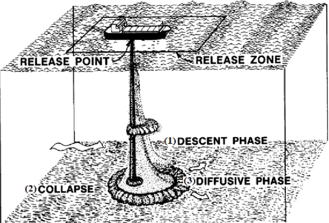
Figure 1-1: The three descent phases of particle clouds during open-water sediment disposal: convective descent, dynamic collapse, and passive diffusion (after Montgomery and Engler, 1986). 25 Figure 1-2: The descent velocity of an idealized particle cloud in the regimes of

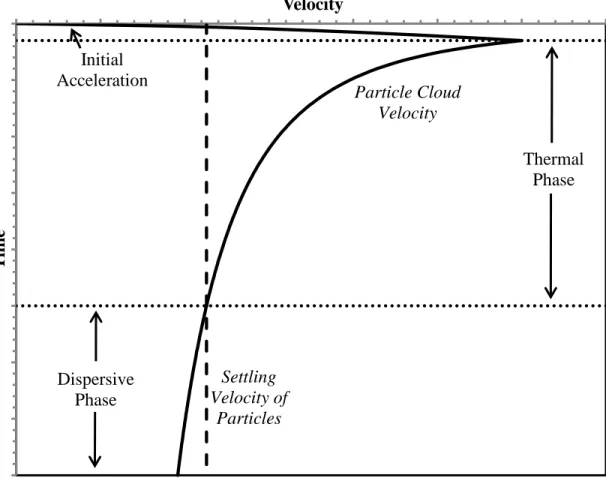
convective descent (after Rahimipour and Wilkinson, 1992; Ruggaber, 2000). 27 Figure 1-3: The different structures of a particle cloud in the self-preserving or

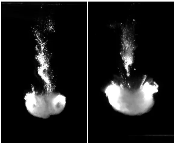
thermal phase: the “parent cloud” (upside-down “cap” on the bottom of each image) and “trailing stem” (top). The particle cloud on the left is composed of larger particles than that on the right. Most of the sediment is usually incorporated into the parent cloud, but the trailing stem is of greater interest in this study because of its susceptibility to being dispersed by ambient currents. 29 Figure 2-1: Two-dimensional cross-sections of vortex rings; the top figure is a

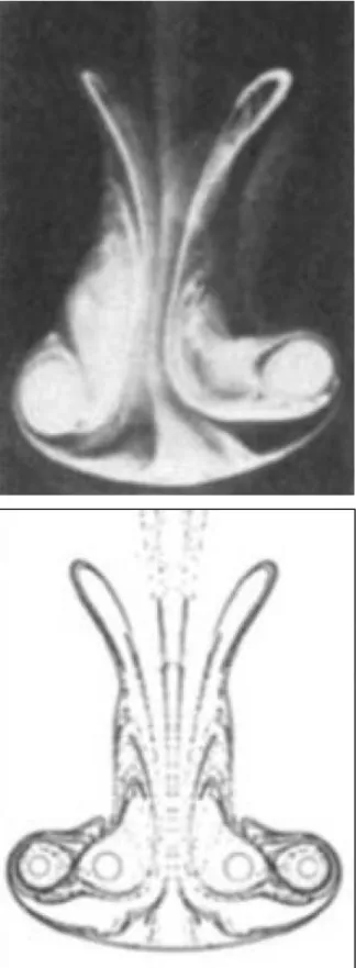
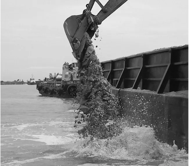
photograph (Yamada and Matsui, 1978) and the bottom image is a computational figure (Shariff, Leonard, and Ferziger, 1989). 39 Figure 3-1: Photograph of a back hoe type dredge, which is an example of a point

release (photo: Z. Huang, 2009). 71

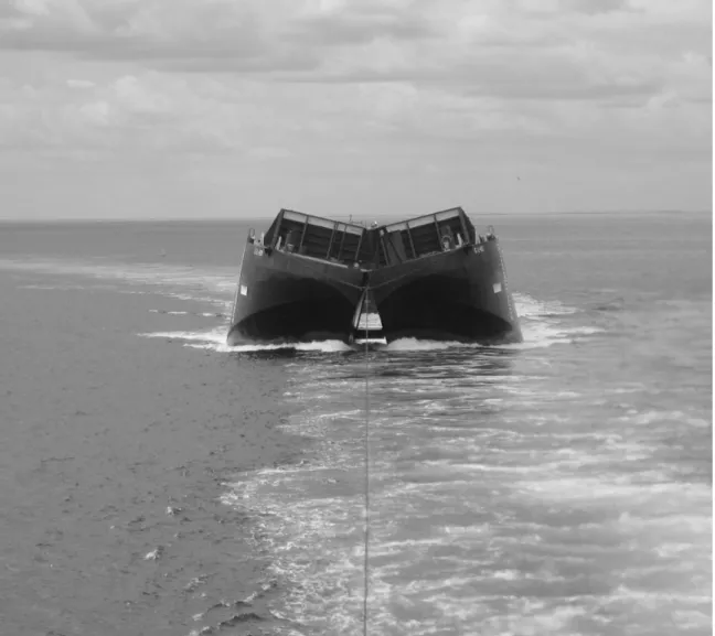
Figure 3-2: Photograph of a split-hull barge, which is an example of a line release

(photo: T. Fredette, 2009). 73

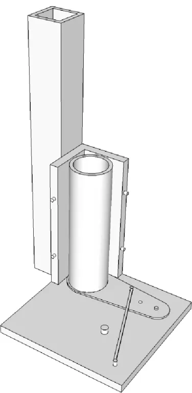
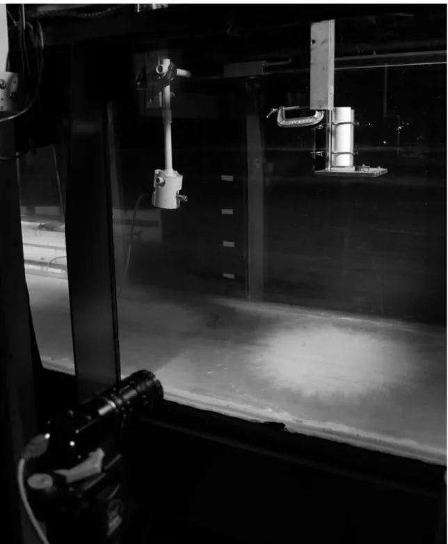
Figure 3-3: The release mechanism used for studying the dynamics of particle clouds released in ambient currents (base is 15.2 cm x 15.2 cm). 77 Figure 3-4: The recirculating channel (shown in the drained condition) with the

laser head, camera, and release mechanism positioned for experimental trials. 81 Figure 3-5: Plan view of the longitudinal grid system used to collect and

(12)

12

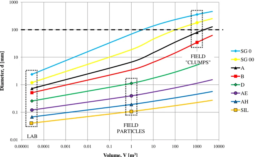
Figure 3-6: Cloud number scaling of the laboratory particles to their relevant field sizes and volumes using a constant release volume in the laboratory (for all particle sizes). Typical field size particles (for a back hoe dredge) and “clumps” (for a split-hull barge) are designated with dashed boxes. 93 Figure 4-1: Qualitative depiction of the evolution of the strength of ambient

currents from “weak” to “transitional” to “strong” as a function of particle size using the coherency of the spherical vortex. The dashed lines show the weak thresholds, and the dotted lines show the strong thresholds for “small” particles (black) and “large” particles (red). 108 Figure 4-2: The weak threshold and strong threshold observations plotted with the

relationships for the critical ambient current velocities, Equations 4-1 and 4-2. 109 Figure 4-3: The descent velocity for five different sizes of particles when released

at the surface in a saturated condition (Note: the descent velocity is found by taking the derivative of the descent of the cloud over time, so a 25-point moving average has been applied to reduce roughness at the local scale; this

averages data points every 0.3125 s). 110

Figure 4-4: Vertical coordinate of the centroid of a descending particle cloud versus time for five different sizes of particles when released at the surface in

a saturated condition. 113

Figure 4-5: Vertical coordinate of the centroid of a descending particle cloud versus parent cloud radius for five different sizes of particles when released at

the surface in a saturated condition. 114

Figure 4-6: Vertical coordinate of the centroid of a descending particle cloud versus time for two different sized particles under two different ambient current velocities when released at the surface in a supersaturated (settled) condition. The open circle shows the pre-release height of the sediment. 116 Figure 4-7: Vertical coordinate of the centroid of a descending particle cloud

versus cloud radius for two different sized particles under two different ambient current velocities when released at the surface in a supersaturated (settled) condition. The open circle shows the pre-release height and radius of

the sediment. 117

Figure 4-8: Longitudinal coordinate of the centroid of a descending particle cloud versus time for when particles were released below the surface into ambient currents of different magnitudes (two different particle sizes). 118

(13)

13

Figure 4-9: Left-to-right from top left: images of Specialty Glass 0, Glass Beads A and AH, and SIL-CO-SIL. The first three are images 1.5 s after release, and the silica image is 3.0 s after release (all releases are saturated and from the surface). The frame size is approximately 40 cm wide x 54 cm tall. 123 Figure 4-10: Vertical coordinate of the centroid of a descending particle cloud

versus time for eight different sizes of particles when released at the surface in a saturated condition. The open circle shows the pre-release height of the

sediment. 125

Figure 4-11: Vertical coordinate of the centroid of a descending particle cloud versus cloud radius for eight different sizes of particles when released at the surface in a saturated condition. The open circle shows the pre-release height

and radius of the sediment. 126

Figure 4-12: Vertical coordinate of the centroid of a descending particle cloud versus cloud radius for B Glass Beads when released at the surface in a saturated condition. The open circle shows the pre-release height and radius of the sediment. The black line shows the two linear regression lines that represent the “turbulent” and “circulating” thermal regimes of descent. 127 Figure 4-13: The thermal created by dense brine when released from the surface;

it has been colored with rhodamine dye to enhance the visualization of the cloud structure. The frame size is approximately 44 cm wide x 55 cm tall. 129 Figure 4-14: Vertical coordinate of the centroid of a descending particle cloud

versus time for two different sizes of particles when released above the surface (dry), at the surface (supersaturated), and below the surface. The open circle shows the pre-release heights of the sediment – all the data have been translated to the surface release height for ready comparison. 131 Figure 4-15: Vertical coordinate of the centroid of a descending particle cloud

versus cloud radius for two different sizes of particles when released above the surface (dry), at the surface (supersaturated), and below the surface. The open circle shows the pre-release heights and radius of the sediment – all the data have been translated to the surface release height for ready comparison. 132 Figure 4-16: Vertical coordinate of the centroid of a descending particle cloud

versus time for two different sizes of particles when released below the surface in quiescent and flowing conditions. The open circle shows the

pre-release heights of the sediment. 133

Figure 4-17: Vertical coordinate of the centroid of a descending particle cloud versus cloud radius for two different sizes of particles when released below

(14)

14

the surface in quiescent and flowing conditions. The open circle shows the pre-release height and radius of the sediment. 134 Figure 4-18: The thermal created by B Glass Beads when released from the

surface in the saturated condition (with rhodamine dye), into a 6 cm/s current. Note the trailing stem as well as the separation of the fluid and particles. The frame size is approximately 31 cm wide x 55 cm tall. 135 Figure 4-19: Vertical coordinate of the centroid of a descending particle cloud

versus time for two different particle sizes when released with three different water contents from the surface: dry, saturated, and supersaturated. The open circle shows the pre-release height of the sediment. 137 Figure 4-20: Vertical coordinate of the centroid of a descending particle cloud

versus cloud radius for two different particle sizes when released with three different water contents from the surface: dry, saturated, and supersaturated. The open circle shows the pre-release height and radius of the sediment. 138 Figure 4-21: An example of a descending particle cloud created with dry, B Glass

Beads that were released at the surface in a 6 cm/s ambient current. 141 Figure 4-22: A simple model of a descending particle cloud. The green regions

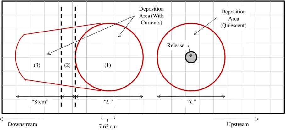
indicate the parts of the parent cloud that land outside the deposition area with a characteristic length equal to a particle cloud descending in quiescent conditions. The red region indicates the part of the trailing stem that will be included in the area designated as the parent cloud, and thus not counted in the first estimate of particle mass in the trailing stem. A “best” estimate of the total mass within the trailing stem is calculated by adding Area (B), as well Area (D) of the parent cloud in exchange for neglecting Area (A). 143 Figure 4-23: Schematic of the two methods of reporting sediment lost to the

ambient environment using the deposition pattern of particles collected from a longitudinal grid on the bottom of the water channel. 147

(15)

15

List of Tables

Table 3-1: Particle types and sizes used to represent both particles and clumps of sediment in experiments modeling open-water sediment disposal. 68 Table 3-2: Cloud number scaling of the laboratory particles to their relevant field

sizes using a constant release volume in the laboratory and realistic release

volumes found in the field. 91

Table 4-1: Group 1 experiments explored the effect of particle size by using

surface releases of saturated sediment. 103

Table 4-2: Group 2 experiments explored the effects of release height, moisture content, and particle condition on glass beads representing field particles (for

a back hoe dredge volume). 104

Table 4-3: Group 3 experiment explored the effects of release height, moisture content, and particle condition on glass beads representing field clumps (for a

split-hull barge volume). 105

Table 4-4: The weak threshold (between “weak” and “transitional” ambient currents) and strong threshold (between “transitional” and “strong” ambient currents) as a function of particle size contained within the particle cloud. 107 Table 4-5: Ratio of the critical ambient current velocity at the weak threshold

between “weak” and “transitional” currents to the maximum descent velocity

of particle clouds. 111

Table 4-6: Ratio of the critical ambient current velocity at the weak threshold between “weak’ and “transitional” currents to the average descent velocity of particle clouds. The fallout depth is calculated using Equation 2-24. 112 Table 4-7: The case and ambient current velocity, u, for the experimental cases of

Gu et al. (2008) compared with the critical ambient current velocities of the weak and strong thresholds, ua,crit,1 and ua,crit,2, using Equations 4-1 and 4-2. 119

(16)

16

Table 4-8: The entrainment coefficients for the “circulating” (𝛼2) thermal regimes of descent for particle clouds composed of eight different particle sizes when released in the saturated condition from the surface. Selected results for Ruggaber’s (2000) most-similar results are shown in the second row, and are

denoted by an “(*)”. 122

Table 4-9: The entrainment coefficients for the “circulating” (𝛼2) thermal regimes of descent for particle clouds composed of two different particle sizes when released at three different elevations: above the surface (dry), at the surface (supersaturated), and below the surface. Selected results for Ruggaber’s (2000) most-similar results are shown in the second row, and are denoted by

an “(*)”. 128

Table 4-10: The entrainment coefficients for the “circulating” (𝛼2) thermal regimes of descent for particle clouds composed of two different particle sizes when released with three different water contents from the surface: dry, saturated, and supersaturated. Selected results for Ruggaber’s (2000)

most-similar results are shown in the second row, and are denoted by an “(*)”. 137 Table 4-11: The total mass collected within the grid and the percentage of mass in

the trailing stem using an underestimate (“1”) and best estimate (“2”) for all Group 2 experiments. Results annotated by (*) are from Ruggaber (2000) for experiments performed with comparable conditions. Results annotated by (**) are overestimates and indicate an upper bound for material in the stem, but the exact amount is unknown because too many particles advected beyond

the grid. 144

Table 4-12: The total mass collected within the grid and the percentage of mass in the trailing stem using an underestimate (“1”) and best estimate (“2”) for all

Group 3 experiments. 145

Table 4-13: The percentage of mass lost to the ambient environment for Group 2 experiments using two definitions for the center of the disposal area. The trials repeated with an (*) are the below surface results that have been adjusted for a change in descent to 55 cm rather than the 60 cm used in other

trials. 149

Table 4-14: The percentage of mass lost to the ambient environment for Group 3 experiments using two definitions for the center of the disposal area. The trials repeated with an (*) are the below surface results that have been adjusted for a change in descent to 55 cm rather than the 60 cm used in other

(17)

17

1 Introduction

This chapter introduces the applications of open-water sediment disposal in the field, provides a brief description of a particle cloud and its descent in a less dense ambient, and outlines the contents included within this thesis.

1.1 Motivation

Open-water sediment disposal is used in many applications associated with both the littoral zones and offshore locations around the world, including land reclamation, coastline extension, dredging, and contaminated sediment isolation (with or without capping). The final example listed is an application of open-water sediment disposal that stems from the significant volume of sediment, particularly contaminated sediment, that is dredged from harbors and navigation channels; in the United States alone, it is estimated that approximately 10 % of the 190 to 230 million m3 of sediment dredged annually contains heavy metals and/or organic chemicals (McDowell, 1999; Suedel et al., 2008). However, its use for all of these functions raises questions concerning the ability to accurately place sediments in a targeted area, as well as the loss of sediments (and potentially contaminants as well) to the ambient environment during disposal operations. Sediment that remains in suspension during disposal introduces additional environmental concerns such as increased turbidity, which adversely affects aquatic vegetation, fisheries, and overall water quality.

(18)

18

Timely and continuing examples of open-water sediment disposal include the land reclamation campaign currently underway in Singapore, as well as the Boston Harbor Navigation Improvement Project of the late 1990s and early 2000s. In the former example, the island nation will soon increase the land area of the country by more than 25 % when compared to its size in the 1960s (Wong, 2005). This equates to more than 100 km2 of land, and creates a requirement for more than 1 billion m3 of sediment to accomplish the task. The latter example is a single illustration of the ongoing trend of ports and harbors around the world increasing navigation depths and maintaining these depths for their approaches, turning basins, and anchorages. The specific example cited in Boston Harbor utilized Confined Aquatic Disposal (CAD) Cells to isolate the approximately 750,000 m3 of contaminated sediment dredged while deepening the harbor’s navigation channels (ENSR, 2002).

These examples, and the volumes of sediment identified, clearly demonstrate the importance of understanding the mechanisms of sediment descent both to dispose sediment accurately, and to minimize sediment losses to the ambient environment. Historical cases in the field have claimed the losses have been minimal, on the order of 1 to 5 % (Truitt, 1988), or have neglected accounting for them at all. Ruggaber (2000) was the first to analyze the physical mechanisms for these losses based on the characteristic cloud behavior as it descended in the water column. In his experiments, he explained the effects of practical release parameters such as release location and moisture content. However, his work was done entirely in quiescent conditions, and in order to extend the applicability and understanding of particle clouds related to open-water sediment disposal, realistic open-water conditions must also be included in the analysis. Most

(19)

19

water bodies are not quiescent, but instead, they are continually under the influence of surface waves and time varying (e.g., tidal) currents; documenting cloud behavior and sediment losses in ambient currents is the focus of this research.

1.2 Description of a Particle Cloud

Sediment that has been released in a sufficiently instantaneous manner in open-water forms a particle cloud, which can be viewed as a sudden release of buoyancy into the surrounding fluid. This assumption makes a particle cloud no different than a heavy fluid with the same density (e.g., a cloud composed of very fine particles would be analogous to a heavy brine). This reduces the particle cloud from a multiphase to a single phase density field, and in the literature this type of sudden release of buoyancy (either lighter or heavier than the surrounding ambient fluid) is called a “thermal” (Scorer, 1957; Woodward, 1959). Depending on the density of the ambient fluid, there can be “light thermals” and “dense thermals.” Hereafter, because open-water sediment disposal involves the release of heavier particles into an ambient fluid with a lower density (i.e., rivers, estuaries, and oceans), the word “thermal” will be used since only “dense thermals” are applicable and therefore discussed.

There are three distinct phases of a descending particle cloud, which are generally also the descriptors given to the behavior of instantaneously released sediment in open-water: 1) convective decent, 2) dynamic collapse, and 3) passive diffusion (Clark et al., 1971; Koh and Chang, 1973; Brandsma and Divoky, 1976; Johnson and Holliday, 1978). A schematic of these three phases of open-water sediment disposal is shown in Figure 1-1, and each phase is summarized below:

(20)

20 1. Convective Descent:

In the first phase, the released sediment forms a particle cloud that resembles a high-density plume. Its downward descent is governed by its negative buoyancy, and ideally, most of the mass is included within the cloud. As the cloud is transported downward, it entrains ambient fluid, decreasing the difference in density between the ambient environment and the particle cloud.

2. Dynamic Collapse:

The second phase is characterized by the collapse of the particle cloud when either it has entrained enough ambient fluid that it reaches a level of neutral buoyancy or the cloud impacts the bottom. As the cloud collapses, the vertical momentum is converted to horizontal momentum, leading to the horizontal spread of the particle cloud.

3. Long-term or Passive Diffusion:

In the final phase, when the dynamic motion and spreading of the particle cloud has ceased, individual particles that formerly made up the cloud advect and diffuse due to ambient currents; their suspended motion depends on the individual settling velocities of the particles (this is independent and unrelated to the third regime of convective descent, which is discussed shortly).

Each phase of open-water sediment disposal is important for understanding the long-term fate of dredged material, but the dynamics of particle clouds and short-term fate of dredged material is encompassed within convective descent. Therefore, the research presented hereafter will focus entirely on the first phase of the descent of particle clouds.

(21)

21

The convective descent phase can be divided into three sub-phases, according to the descent velocity of the particle cloud: 1) initial acceleration phase, 2) thermal phase, and 3) dispersive phase (Rahimipour and Wilkinson, 1992; Noh and Fernando, 1993). These regimes are shown in Figure 1-2 and are described in greater detail below:

1. Initial Acceleration Phase:

Prior to a particle cloud release, the particles are closely packed and at rest. Upon release, the sediment (or sediment/fluid mixture if it contains water) accelerates and expands rapidly. Ambient water is entrained, in part due to the shearing effect at the edge of the cloud which produces turbulent instabilities and disperses the particles. The entrainment reduces the difference in density between the cloud and the ambient environment, and after reaching its maximum velocity, the cloud begins to decelerate and enters the second phase.

Theoretical (Escudier and Maxworthy, 1973) and experimental (Baines and Hopfinger, 1984) investigations have demonstrated that the initial acceleration phase is a function of the initial buoyancy, and that its length for a thermal is approximately equivalent to 1 to 3 initial cloud diameters. Later studies on dense thermals (Neves and Almeida, 1991) have generally confirmed these results, and similar development scales have been recorded by numerical studies for particle clouds, and confirmed by experimental findings (Li, 1997).

2. Self-Preserving or Thermal Phase:

As the density of the particle cloud continues to decrease (as the less dense ambient fluid is entrained into it), thermals and particle clouds asymptotically decelerate. It is assumed that this self-preserving phase has been reached when i) the

(22)

22

transverse profiles of vertical velocity and buoyancy are similar at all depths, and ii) the rate of entrainment of fluid as a function of depth is proportional to the characteristic velocity for the same observed depth (Batchelor, 1954; Morton, Taylor, and Turner, 1956). As eddies on the boundary grow, and correspondingly more ambient fluid is entrained into the aft (top) of the cloud, the cloud evolves into an axisymmetric vortex ring, or spherical vortex described by Hill (1894). During this evolution, the distribution of buoyancy shifts from its original profile of a Gaussian-type, to one that is bimodal (due to the shift of the maximum from the center of the cloud to the centers of the vortex rings when looking at a two-dimensional cross section of the spherical vortex). The spherical vortex continues to entrain fluid and re-entrain particles from the stem (particles that were not originally incorporated into the cloud; this will be developed in more detail later) down through the center of the cloud, and an upflow exists on the outside of the cloud. This leads to greater horizontal spreading, or flattening, of a particle cloud, and causes the cloud to resemble an upside-down mushroom-shaped thermal.

Ruggaber (2000) demonstrated that the thermal phase of particle clouds can also be subdivided into what he called “turbulent thermals” and “circulating thermals.” These two regimes correspond to the absence and presence of the spherical vortex, respectively, in the transition discussed above. For non-cohesive sediment, this evolution is marked by the change from large growth rates (𝛼 = 0.2 to 0.3), where 𝛼 is the entrainment coefficient, to linear growth rates (𝛼~ 𝐵 𝐾 ) consistent with 2

buoyant vortex ring theory (where B is the buoyancy of the particle cloud; and K is the cloud circulation). The transition was observed when the radius of the particle

(23)

23

cloud had reached a value four times greater than its initial pre-release radius (Ruggaber and Adams, 2000). Thermal and buoyant vortex ring theory (including the entrainment coefficient) is explained in more detail in Chapter 2.

3. Dispersive or Particle-Settling Phase:

In the final phase of convective descent, the deceleration of the particle cloud eventually reduces the descent velocity of the thermal to a value comparable to the settling velocity of individual particles within the particle cloud. As this occurs, the internal motion of the thermal is suppressed and insufficient to hold the particles in suspension, and the individual particles all move downward and “rain out” of the neutrally buoyant cloud at a nearly constant velocity. These settling particles are collectively called a “swarm” (Bühler and Papantoniou, 1991; 2001; Bush, Thurber, and Blanchette, 2003) or “cluster” (Slack, 1963; Bühler and Papantoniou, 1999) that is bowl-shaped and continues to expand due to the weak dispersive forces between adjacent particles (Rahimipour and Wilkinson, 1992) or to the shear induced outward diffusion of turbulence and lateral displacement flow caused by the wake of each particle (Bühler and Papantoniou, 2001).

This study focuses on the second phase, the thermal phase, of descent because of its applicability to a wide range of depths for open-water sediment disposal. The initial acceleration phase lasts for a short period of time, and the dispersive phase is reached for greater depths than those being investigated. In the self-preserving or thermal phase, most of the sediment is incorporated in the axisymmetric upside-down mushroom cloud, or self-similar “cap,” or “parent cloud.” However, some sediment is also contained in an irregular “trailing stem.” Figure 1-3 shows the distinction between the parent cloud and

(24)

24

trailing stem using photographs taken during two different experimental trials. Although most sediment is incorporated into the parent cloud, the trailing stem is also of interest because this material is more easily dispersed by currents and waves; further, the concentration of pollutants may be higher than in the parent cloud due to the generally finer particle composition. The terms “parent cloud” and “trailing stem” will be used throughout the rest of this thesis to refer to the two distinct structures that make up a particle cloud.

(25)

25

Figure 1-1: The three descent phases of particle clouds during open-water sediment disposal: convective descent, dynamic collapse, and passive diffusion (after Montgomery and Engler, 1986).

(26)

(27)

27

Figure 1-2: The descent velocity of an idealized particle cloud in the regimes of convective descent (after Rahimipour and Wilkinson, 1992; Ruggaber, 2000).

T im e Velocity Particle Cloud Velocity Settling Velocity of Particles Initial Acceleration Thermal Phase Dispersive Phase

(28)

(29)

29

Figure 1-3: The different structures of a particle cloud in the self-preserving or thermal phase: the “parent cloud” (upside-down “cap” on the bottom of each image) and “trailing stem” (top). The particle cloud on the left is composed of larger particles than that on the right. Most of the sediment is usually incorporated into the parent cloud, but the trailing stem is of greater interest in this study because of its susceptibility to being dispersed by ambient currents.

(30)

(31)

31

1.3 Overview of Thesis Contents

This thesis will review thermals and buoyant vortex rings as they apply to particle clouds, and the methods used to relate the particle clouds created in the laboratory to the real world will be explained. Further, the following questions will be investigated:

 How do the release variables that are seen in the field (i.e., release height – initial momentum, water content – sediment moisture, and particle size and compaction) influence the creation of the self-similar thermal?

 How do self-similar particle clouds created in quiescent conditions compare to those in ambient currents? Is there a threshold above which the ambient current is too strong for the thermal to develop?

 Do the basic characteristics of particle clouds such as growth rate and descent depend on the release variables, and are these patterns consistent with and without the presence of ambient currents?

 Does an ambient current amplify the potential for more sediment to be left out of the parent cloud (therefore increasing the fraction of mass found in the trailing stem)?

 Can ambient currents increase the total sediment losses to the ambient environment? Do these losses originate from material that in the thermal phase of descent were originally within the parent cloud, the trailing stem, or both?

 Are losses to the water column consistent as a function of the magnitude of the ambient current? Are reasonably low percentages of particle cloud losses measured in similar time windows that are currently designated by regulatory agencies?

(32)

(33)

33

2 Theory and Background

This chapter provides additional information on previous studies of thermals, buoyant vortex rings, and particle clouds. Ruggaber (2000) performed a rigorous review of thermals, buoyant vortex rings, and particle clouds, and the historical (more than a decade since) literature review portions of the first three sections of this chapter largely summarize his work. Other sections and subsections provide additional details on laboratory particle cloud studies as they relate to open-water sediment disposal, as well as field cases that highlight the short-term fate of dredged material following open-water sediment disposal; the primary focus of the field cases that have been selected is on the aspect of their investigations which concentrated on quantifying sediment losses.

2.1 Thermals

Because the second phase of convective descent for particle clouds resembles the classical thermal, it is pertinent to review the theory of classical thermals and studies of them which have been performed in the recent past.

2.1.1 Theoretical Analysis of Thermals

A number of researchers have analyzed thermals using numerical models that are formulated on the basis of the conservation equations (i.e., mass, momentum, and buoyancy), including Koh and Chang (1973), Li (1997), and many others. Koh and

(34)

34

Chang (1973) implemented an integral analysis by treating the thermal as a descending, expanding control volume, and in doing so, arrived at the following conservation equations: Conservation of Mass: 𝑑 𝑑𝑡 𝜌𝑟 3 _{= 3𝛼𝜌} 𝑎𝑟 2_𝑤 (2-1) Conservation of Momentum: 𝑑 𝑑𝑡 𝑉 𝜌 + 𝑘𝜌𝑎 𝑤 = 𝐵 − 0.5𝜌𝑎𝐶𝐷𝜋𝑟 2_𝑤2 (2-2) Conservation of Buoyancy: 𝑑 𝑑𝑡 𝐵 = 𝑑 𝑑𝑡 𝑉 𝜌 − 𝜌𝑎 𝑔 = 0 (2-3)

where  is the density of the thermal; a is the density of the ambient fluid; r is the

thermal radius; w is the mean descent velocity of the thermal centroid; α, k, and CD are

the entrainment, added mass, and drag coefficients, respectively; V is the thermal volume; B is the thermal buoyancy; and g is the gravitational constant. Equation 2.1 makes Sir Geoffrey Taylor’s basic entrainment assumption that the mean inflow velocity is proportional to w, and Equation 2.3 assumes that no buoyancy is lost to the environment outside the control volume (e.g., the thermal wake). If the densities of the thermal and the ambient fluid are assumed to be approximately equal (i.e., a Boussinesq approximation), and if 𝑤 =𝑑𝑧_𝑑𝑡, then:

(35)

35

where z is the vertical position of the particle cloud’s center of mass. The continuity equations and entrainment assumption result in a linear relationship between the thermal radius and its vertical position.

By building upon the dimensional analysis solutions by Batchelor (1954), the following similarity solutions were derived by Turner (1973) by neglecting viscosity and pressure for an axisymmetric turbulent thermal suddenly released into an environment of a uniform density: 𝑟 = 𝛼𝑧 𝑤 = _𝜌𝐵 𝑎 1 2 𝑧−1_𝑓 1 𝒓_𝑟 (2-5) 𝑔′ = 𝐵 𝜌_𝑎 𝑧−3𝑓2 𝒓 𝑟

where r is the vector position from a vertical line below the source (axis of symmetry); g’ r

is the modified gravitational constant, 𝜌−𝜌_𝜌 𝑎

𝑎 𝑔; and f1 and f2 are profile functions. By

once again setting 𝑤 =𝑑𝑧

𝑑𝑡 and also neglecting the distribution of velocity and buoyancy

within the thermal, the following time dependencies are realized:

𝑟 ~ 𝛼 _𝜌𝐵 𝑎 1 4

_𝑡

1₂ ; 𝑤 ~ _𝜌𝐵 𝑎 1 4

_𝑡

− 1₂ (2-6)

Using a simplified model, both Wang (1971) and Escudier and Maxworthy (1973) derived solutions to the three conservation equations for the initial accelerating motion and final decelerating motion of a buoyant thermal. In both investigations, the asymptotic solutions were conceived by first non-dimensionalizing the length (𝑟 ), time (𝑡 ), and velocity (𝑤 ) scales:

(36)

36 𝑟 =_𝑟𝑟 𝑜 𝑡 = 𝑡 𝑔∆_𝑟𝑜𝛼 𝑜 1 2 (2-7) 𝑤 = 𝑤 𝛼 𝑟_𝑜𝑔∆_𝑜 1 2

where ∆_𝑜 is the initial buoyancy, 𝜌𝑜_𝜌−𝜌𝑎

𝑎 ; and ro is the initial length scale. By neglecting

the drag forces and invoking the same assumption as made in Equation 2.3 for a spherical thermal, Escudier and Maxworthy (1973) reported the asymptotic solutions shown below:

Short times: 𝑟 − 1 ≪ 1 𝑟 − 1 ≈_{2 1+𝑘 −∆}𝑡2 𝑜 ; 𝑤 ≈ 𝑡 1+𝑘−∆_𝑜 (2-8) Long times: 𝑟 − 1 ≫ 1 𝑟 − 1 ≈ 𝑡 1 2 2 1+𝑘 14 ; 𝑤 ≈ 𝑡−12 234 1+𝑘 14 (2-9)

When Equation 2.9 is returned to dimensional form, it is similar to Equation 2.6, except for the presence of constants and the inclusion of the added mass coefficient. The result is below: 𝑟 = _4𝜋𝜌3𝛼𝐵 𝑎 1 4 𝑡12 2 1+𝑘 14 ; 𝑤 = _4𝜋𝜌3𝐵 𝑎 1 4 𝑡− 12 2𝛼 34 1+𝑘 14 (2-10)

Baines and Hopfinger (1984) performed a study on thermals with large density differences (i.e., the density of the thermal and the ambient fluid are not equal), thus removing the linear correlation between the thermal radius and vertical position. The relationship they developed specifically includes a ratio of densities:

(37)

37 𝑟 = 𝛼𝑧 𝜌_𝜌𝑎

1 3

(2-11)

The inclusion of and dependence of the thermal radius on the ratio of the ambient density to the thermal density is due to the high rate of entrainment of ambient fluid. As a result, the Boussinesq approximation is reached nearly immediately after the release of a thermal; Baines and Hopfinger concluded from theoretical and experimental analyses that for a dense thermal, the Boussinesq approximation was reached after the descent of approximately four initial radii (and even sooner for a rising, light thermal).

2.1.2 Laboratory Studies of Thermals

The principal experiments on buoyant thermals concentrated on light thermals in the 1950s and 1960s as researchers were motivated to understand the fluids of meteorological phenomena such as heat convection; later, dense thermals were also investigated for the purpose of understanding the descent of dredged material. For these studies that specifically analyze particle clouds, details of the investigations are included in Section 2.3. However, dense thermals can also be created with dense solutions such as brine. This was done by Richards (1961) when he released a thermal of brine from a hemispherical cup into a step-stratified mix of freshwater and salt water. Using dimensional analysis, Richards associated its descent and entrainment as follows (for while the thermal remained in the upper, freshwater layer):

𝑧2 _{= 𝑐} 1𝛼−

3 2 𝐵

𝜌_𝑎 𝑡 (2-12)

The experiments recorded a wide range of entrainment values, from 0.13 to 0.50. Further, Richards concluded that there was not any evidence of a relationship between the

(38)

38

configuration of the release and the resulting value of α, but that the speed of the inversion of the release cup did affect the resulting α. Particularly, at times if it was slow enough to induce more of a pour-like condition, then a plume resulted instead of a thermal. However, for this wide range of entrainment values, he found that c1 = 0.73 for

nearly all of the thermals he produced in the given set of experiments. Turner (1964) confirmed that the dependence of c1 on α is small, finding a value of 0.69, but reported a

slight dependence on the shape and angle of spread of the thermal and added mass coefficient.

2.2 Buoyant Vortex Rings

The evolution of a particle cloud from, using terms that Ruggaber (2000) coined, the “turbulent thermal” to the “circulating thermal” includes the formation of a buoyant vortex ring. These have been studied for more than a century; hence, the pertinent details of them are included in this section. A photograph of the two-dimensional cross-section of a vortex ring is shown in Figure 2-1 as a reference.

2.2.1 Theoretical Analysis of Buoyant Vortex Rings

The discussion of thermals above focused on the sudden release of buoyancy into a less dense ambient. Buoyant vortex rings also progress under the influence of buoyancy, but in addition to buoyancy, they also require momentum, or impulse (I), and circulation (K) to be initiated. Lamb (1932) performed a rigorous mathematical review of the hydrodynamic impulse and circulation of many varieties of vortices, including the vortex ring. These mathematical expressions can be used to deduce characteristics of the

(39)

39

Figure 2-1: Two-dimensional cross-sections of vortex rings; the top figure is a photograph (Yamada and Matsui, 1978) and the bottom image is a computational figure (Shariff, Leonard, and Ferziger, 1989).

(40)

(41)

41

buoyant vortex ring, and one of note is the vertical velocity of the vortex ring, wvr, which

Turner (1957) wrote by assuming similarity and is shown below: 𝑤_𝑣𝑟 = 𝑐 𝐾

𝑟 (2-13)

where c is a constant that varies based on the shape of the vortex ring; and r is the mean radius of the torus (equivalent to the previously defined radius of the thermal).

Saffman (1995) published an overview of vortex dynamics, which he hoped would serve as an updated reference on vortex motion presented in Chapter VII of Lamb’s Hydrodynamics (1932). Saffman’s review of vorticity and vortex rings, lines, sheets, and patches is thorough, and he also included Hill’s (1894) spherical vortex and the axisymmetric vortex ring, which is of the most interest in this research. This is an example of a vortex jump, where the vorticity is confined within a uniform sphere translating through an ambient fluid; outside the sphere, flow is irrotational. When determining the distribution of vorticity, one can assume that at a particular instant, the origin of a cylindrical polar coordinate system, 𝑏, 𝜃, 𝑦 , is at the center of the sphere, and the distribution of vorticity, 𝝎, is equal to 0, 𝜔_𝜃, 0 . For a constant A:

𝜔𝜃 = 𝐴𝑏, 𝑏2+ 𝑦2 < 𝑎2; 𝜔𝜃 = 0, 𝑏2+ 𝑦2 > 𝑎2 (2-14)

where a is the radius of the sphere. From this, the velocity field can be determined, which due to the axisymmetric characteristic of the spherical vortex, can be described using a Stokes stream function. The pressure can be found using Bernoulli, and when an additional pressure term, 2𝐴𝜇𝑦, is added inside the sphere to account for viscosity, the velocity field also satisfies the Navier-Stokes equations both inside and outside the spherical vortex.

(42)

42

2.2.2 Laboratory Studies of Buoyant Vortex Rings

Turner (1957) assumed a constant circulation and that the buoyancy increases the impulse of a ring in a uniform ambient fluid. In addition to theoretically analyzing the velocity of a vortex ring, he formulated a new linear relationship between the radius and vertical location based on a new entrainment coefficient:

𝑟 = 𝛼′𝑧 (2-15)

or

𝛼′ ₌ 𝐹

2𝜋𝑐𝐾2 (2-16)

where F is the ratio of buoyancy to the density of the ambient fluid and remains constant. This complicates the entrainment, since the circulation is actually produced by the buoyancy, thus making assumptions such as a uniform environment and constant circulation convenient. Realistically, this only applies well after the initial acceleration phase when a thermal has reached the circulating thermal phase. Turner produced vortex rings in experiments in a glass tank with a depth of approximately 1.52 m by forcing dyed fluid into the tank. He found values of c that ranged between 0.13 and 0.27, and observed that the motion became stable at a density difference of 4 %. These experimental results were visited again by Turner (1960) for further analysis with vortex pairs, particularly experiments which he had also previously performed in stratified environments. These experiments had an increased density difference as high as 18 % (Turner, 1957).

Maxworthy (1974) used a piston to eject a finite mass of fluid through a sharp-edged orifice. This created a turbulent vortex ring, which Maxworthy determined had an entrainment coefficient with a value of 0.011 ± 0.001. He also found that the effective

(43)

43

drag coefficient for an equivalent spherical volume was 0.09 ± 0.01. Maxworthy believed that both of these experimental results were independent of Reynolds number.

In a second set of experiments designed to analyze vortex rings at high Reynolds number (Re = 103 to 105), Maxworthy (1977) used both flow visualization and laser-Doppler techniques in a larger tank with a length of 2 m. He found that the formation process was actually highly Reynolds number dependent, and additionally, made qualitative observations of the “organization” of the vortex core which heavily influenced the growth of the vortex ring. The “well-organized” rings, with the clear core and outer-flow interfaces, experienced lower growth rates (α = 0.001). The “disorganized” rings had entrainment values more than an order of magnitude larger (α = 0.015), and Maxworthy hypothesized that this was due to the relative level of turbulence between the vortex ring and the ambient fluid.

Sau and Mahesh (2008) numerically simulated the dynamics of vortex rings when injected into a cross-flow, with an interest in fuel injectors, turbojets, and other high velocity injectors. When compared to the quiescent ambient condition, in a cross-flow a coherent vortex ring lost its symmetry or did not form at all, depending on the velocity ratio and the stroke ratio. The velocity ratio is defined as the ratio of the average nozzle exit velocity to the free stream cross-flow velocity; the stroke ratio is defined as the ratio of the stroke length to the nozzle exit diameter (i.e., an aspect ratio). Below velocity ratios of approximately two, a vortex ring was not formed, but instead, a hairpin vortex formed. Above velocity ratios of two with a low stroke ratio, a coherent asymmetric vortex ring was formed; however, for larger stroke ratios the vortex ring was trailed by a column of vorticity. In both cases, the vortex ring adopted a “tilt.” In the former case,

(44)

44

the vortex ring tilted downstream, whereas in the latter case with the trailing vorticity, the vortex ring tilted upstream. In general, Sau and Mahesh also confirmed that a larger stroke ratio enhanced mixing and entrainment, which was partially due to the trailing vorticity.

2.3 Particle Clouds

Particle clouds have been studied both experimentally in the laboratory and with numerical modeling. In the past two decades, the focus has remained finding a greater understanding of the behavior of particle clouds (e.g., growth and circulation) and the transition depths between their different phases. Summaries of many of these investigations are included in this section.

Tamai, Muraoka, and Murota (1991) studied two-dimensional (i.e., line) releases of particle clouds which result from split-hull barges in the field. They used a mixed sand that was composed of two uniform grain sizes, a fine sand (d50 = 0.15 mm) and a

coarse sand (d50 = 3.38 mm). The sand was dumped from an acrylic box with a width of

5 cm and an opening time of 0.3 s into a flume. When the mixture was released together, the coarser sand settled on the bottom while the finer sand remained in suspension and formed what the authors called a “turbidity cloud.” Additional experiments studied releases with only the coarse sand and found that qualitative characteristics such as the linear growth rate and descent velocity as a function of time were similar to turbulent thermals formed by an instantaneous discharge of buoyancy.

Rahimipour and Wilkinson (1992) analyzed particle clouds using sheet illumination in order to expose the internal structure of particle clouds composed of

(45)

45

graded sand ranging in diameter from 0.150 mm to 0.350 mm. Various experiments were performed to capture the descent velocity of particle clouds composed of different particle sizes and initial volumes, and the authors found that these velocities were comparable to those found for a miscible thermal of the same size and buoyancy. These comparisons were based on the use of the cloud number, which Rahimipour and Wilkinson defined as the ratio of the individual particle settling velocity to the characteristic thermal descent velocity; the cloud number is shown in its “local” form below:

𝑁_𝑐 = 𝑤𝑠𝑅

𝐵 𝜌 _𝑎

1

2 (2-17)

where ws is the settling velocity of the individual particles; R is the local radius of the

particle cloud (i.e., at a particular time or depth); B is the buoyancy of the particle cloud; and a is the density of the ambient fluid. The descent velocities were most similar for a

particle cloud and a miscible thermal for small values of the cloud number, Nc. However,

as the cloud continued to descend (and the local cloud number increased with the size of the cloud), and particularly following the raining out of individual particles, there was a greater discrepancy between the velocity of the “swarm” and that of a miscible thermal.

Using this information, Rahimipour and Wilkinson developed the following relationship between the entrainment coefficient and the cloud number:

𝛼 = 0.31 1 − 0.44𝑁_𝑐1.25 𝑓𝑜𝑟 𝑁_𝐶 < 1 (2-18) The relationship above fulfilled the authors’ observation that for small values of the cloud number (Nc < 0.3), the growth and entrainment rates of particle clouds was the same as

(46)

46

number; this was specifically observed when Nc > 1. Once the cloud number was greater

than 1.5, the growth slowed enormously. Thus, in the final phase a cloud’s radius can be described by the following relationship:

𝑅 = 1.5 _𝜌𝐵 𝑎

1

2 1

𝑤𝑠 𝑓𝑜𝑟 𝑁𝑐 > 1.5 (2-19) Noh and Fernando (1993) investigated the two-dimensional characteristics of particle clouds released into water to determine the transition between which particle clouds form a descending thermal and individual particles settle as a swarm. Particles were released using a two-dimensional funnel that was triangular in cross section but was 15.3 cm in length, therefore creating a two-dimensional particle cloud (i.e., a line release). Glass beads and 50 ml of water with fluorescein were added to the funnel and released into a rectangular tank with a depth of 111.9 cm. The particles had mean diameters of 0.080 mm, 0.240 mm, 0.510 mm, and 0.720 mm. The authors found that, initially, the particle/fluid mixture created a particle cloud resembling a thermal, but eventually, the particles settled out of the dyed water, creating a bowl-shaped swarm. Meanwhile, the fluid cloud showed signs of decaying turbulence and vortices.

The authors found that for experiments with the various particle sizes, the transition between the self-similar thermal and dispersive phases of descent occurred at a critical fallout depth, zf, which is defined by:

𝑧_𝑓𝑤_𝑠 𝜈

~

𝑄 𝜈𝑤_𝑠 𝛼 𝑤𝑖𝑡𝑕 𝛼 ≅ 0.3 (2-20) where Q is the total buoyancy of the particle cloud; ν is the kinematic viscosity of the ambient fluid; and zf is the depth measured from the surface to the frontal position of the

(47)

47

Fernando speculated that previous assumptions about the transition being wholly dependent on particle size, or of a related quantity, that determines the particle settling velocity, were incomplete. The authors hypothesized that the accepted transition between the second and third phases of convective descent, when wc ~ ws, where wc is the descent

velocity of the particle cloud, can fluctuate around this approximation in the presence of ambient turbulence or fluid motion. This would theoretically allow a particle cloud to remain in the thermal phase when wc < ws, but this could not be observed in this study.

Johnson and Fong (1995) carried out experiments using sand, silt, clay, and fine crushed coal at the U.S. Army Corps of Engineers’ Waterways Experiment Station by modeling a split-hull barge and hopper dredge on a 1:50 scale. By performing tests in water depths ranging from 0.61 m to 1.83 m and focusing on the phase following convective descent, dynamic collapse, the authors developed a numerical model called STFATE (Short-Term FATE). This model made widespread revisions to a previous mathematical model originally developed by Koh and Chang (1973). STFATE can be used for calculating the water column concentrations and bottom deposition that result from the disposal operations of dredged material. The authors concluded that STFATE reproduced the fate of dredge material disposed in open water with an acceptable error. They found that the average simulated and measured descent speeds had percentage differences less than 25 %, and the average bottom surge speeds varied by approximately 10 %. The model also calculated that 2 to 3 % of the original material for silt and clay disposals was stripped from the parent cloud during descent.

Li (1997) performed a numerical study that investigated the motion induced by a finite release of particles that are heavier than the stagnant fluid into which they are

(48)

48

released by using a three-dimensional numerical model that was based on the conservation of mass, momentum, and density excess. The model was valid as long as the particles could be characterized by a single, continuous field of density difference with a specific settling velocity, and also assuming that the Boussinesq approximation was valid. Using the cloud width as the length scale for the mixing length, Li’s model reproduced the bimodal distribution of buoyancy, but only for particle sizes ranging from 0.15 mm to 0.30 mm. For larger particle sizes (0.6 mm to 1.18 mm), coherent vortex rings were not simulated by the model.

Ruggaber (2000) performed flow visualization experiments using silt and non-cohesive glass beads of various sizes that were released quasi-instantaneously into a glass tank nearly 2.5 m deep. His focus was to study how realistic modes and variables of sediment disposal operations (e.g., particle size, water content, and initial momentum) affected cloud behavior (i.e., particle cloud descent velocity, growth rate, and loss of particles) and the entrainment (𝛼), drag (CD), and added mass (k) coefficients as a

function of time. By holding the dry release mass constant (40 g), he was able to use the laboratory release volume and realistic volumes in field operations to scale the particles to field size by employing the cloud number (more on the specifics of this scaling is explained in Section 0). Ruggaber found that the releases of cohesive sediment produced a wide range of growth rates, but the non-cohesive releases closely following the theoretical phases of convective descent. Initially, thermals were promptly developed, which was followed by an asymptotic deceleration and large growth rates (𝛼 = 0.2 to 0.3). Then, the growth slowed greatly once the circulation increased,

(49)

49

corresponding to the presence of a buoyant vortex ring. For large particles (Nc > 10-4),

the growth was reduced to 𝛼 = 0.1 to 0.2.

Ruggaber also used his experimental results to calibrate an “inverse” integral model which employed the conservation equations in order to find 𝛼 and k using measured data from the particle cloud experiments (i.e., descent velocity and radius). He found that in the thermal phase, CD and k are nearly zero. Conversely, once particle

clouds transitioned to a “circulating thermal,” the significant reduction in growth, 𝛼, caused by larger particles (when the cloud number is greater than 10-4), increased k to a value similar to a solid sphere. These results demonstrated that constant values are appropriate for smaller particle sizes, but when Nc > 10-4, time varying coefficients are

required to properly document the cloud behavior. Ruggaber was also the first to quantify the difference between the parent cloud and trailing stem using a sediment capture mechanism that he suspended within the tank, and this will be discussed more in the next section.

Bühler and Papantoniou (2001) presented methods that predicted the growth and velocity of particle clouds for both the thermal and swarm regimes of decent. In addition to using theoretical relationships, experiments were performed to determine the constants in these relationships. These experiments were carried out in a tank with a depth of 1.1 m by releasing particles through a funnel positioned near the water surface. These particles ranged in size for one series of tests from 1.5 mm to 2 mm, and for a second series of tests they ranged from 2 mm to 3 mm. The particle clouds were illuminated from below using a light sheet, and tests were performed with different thermal buoyancies (i.e., different

(50)

50

initial mass of particles). The front velocity and width of the particle clouds were determined by using video frames that were captured at intervals of 4/25 s.

For their theoretical analysis, Bühler and Papantoniou retained earlier expressions that the transition between the thermal and swarm stages occurred when the velocity of the particle cloud front is comparable to the settling velocity of individual particles:

𝑤𝑓 = 𝑐𝑠𝑤𝑠 (2-21)

where wf is the velocity of the front of the particle cloud; and cs is a constant found with

experiments; the experiments described above determined this value to be 1.4. When Equation 2-21 is used, the authors expressed the transitional depth between descent regimes as: 𝑧_𝑓 = _𝑐𝑐𝑇 𝑠𝑤𝑠 𝐵 𝜌_𝑎 1 2 (2-22)

where cT is a constant (equal to 2.6 for a spherical shape and 2.94 for a spheroid shape).

Bush, Thurber, and Blanchette (2003) conducted experiments by releasing heavy particles (i.e., glass spheres ranging in size from 0.002 cm to 0.1095 cm) into both homogeneous and stratified ambient environments (i.e., a cylindrical tank with a depth of 90 cm that was filled with either water or salt water with a linear stratification). Particle releases had various dry weights from 0.2 g to 50 g and also contained small amounts of water (5 ml to 10 ml). Flow visualization was enhanced using food coloring dyes and fluorescein. For the releases performed in the homogeneous ambient, the investigators found that the particle clouds evolved into the three clear phases of a classical fluid thermal discussed in Chapter 1. Although the transition between the initial acceleration phase and self-similar thermal phases was not initially clear, the transition between the

(51)

51

second phase and the dispersive phase was obvious. The second transition was quantified using the particle Reynolds number, Rep, which the authors defined as:

𝑅𝑒_𝑝 = 𝑤𝑠_𝜈𝑟𝑠 (2-23)

where rs is the radius of the individual particles. For values in the range of 0.1 to 300, the

fallout height of individual particles in the dispersive phase into the bowl-shaped swarm (measured depth since release), zf, was found to be:

𝑧_𝑓 𝑟_𝑠 = 11 ± 2

𝑄1 2 𝑤_𝑠𝑟_𝑠 5 6 (2-24)

For higher particle Reynolds numbers (Rep > 4), the relationship could be simplified and

depended exclusively on the number and size of particles released, and it assumed the form:

𝑧𝑓 = 9 ± 2 𝑟𝑠𝑁𝑃12 (2-25)

where NP is the number of particles released.

Bush et al. also found a correlation between initial buoyancy (in the form of total initial payload, or mass of particles released), and the length of the initial acceleration phase. Although the rate of growth or expansion of the cloud is ultimately independent of the initial payload mass (𝛼 ~ 0.25), when comparing trials with initial masses ranging from 1.0 g to 20.0 g, the latter cases traveled a greater distance z from the point of release for the thermal-like flows to be established. The authors concluded that the entrainment coefficient 𝛼 had no dependence on the Rayleigh number and potentially had a weak dependence on the particle Reynolds number (they also suggested that it could be approximated by a mean constant value, even with its dependence on Nc). Bush et al.