Probability distributions of wind speed in the UAE.

1

Probability distributions of wind speed in the UAE

1

2

T.B.M.J. Ouarda

, C. Charron

, J.-Y. Shin

, P.R. Marpu

, A.H. Al-Mandoos

,

M.H. Al-Tamimi

, H. Ghedira

and T.N. Al Hosary

5 1

Institute Center for Water and Environment (iWATER), Masdar Institute of Science and 6

Technology, P.O. Box 54224, Abu Dhabi, UAE 7

2

INRS-ETE, National Institute of Scientific Research, 490 de la Couronne, Quebec City (QC), 8

Canada, G1K9A9 9

3

National Centre of Meteorology and Seismology, P.O. Box 4815, Abu Dhabi, UAE 10 11 *Corresponding author: 12 Email: touarda@masdar.ac.ae 13 Tel: +971 2 810 9107 14 15 16

Submitted to Energy Conversion and Management 17

December 2014 18

2

Abstract

19

For the evaluation of wind energy potential, probability density functions (pdfs) are usually used 20

to describe wind speed distributions. The selection of the appropriate pdf reduces the wind power 21

estimation error. The most widely used pdf for wind energy applications is the 2-parameter 22

Weibull probability density function. In this study, a selection of pdfs are used to model hourly 23

wind speed data recorded at 9 stations in the United Arab Emirates (UAE). Models used include 24

parametric models, mixture models and one non-parametric model using the kernel density 25

concept. A detailed comparison between these three approaches is carried out in the present 26

work. The suitability of a distribution to fit the wind speed data is evaluated based on the log-27

likelihood, the coefficient of determination 2

R , the Chi-square statistic and the Kolmogorov-28

Smirnov statistic. Results indicate that, among the one-component parametric distributions, the 29

Kappa and Generalized Gamma distributions provide generally the best fit to the wind speed data 30

at all heights and for all stations. The Weibull was identified as the best 2-parameter distribution 31

and performs better than some 3-parameter distributions such as the Generalized Extreme Value 32

and 3-parameter Lognormal. For stations presenting a bimodal wind speed regime, mixture 33

models or non-parametric models were found to be necessary to model adequately wind speeds. 34

The two-component mixture distributions give a very good fit and are generally superior to non-35

parametric distributions. 36

Keywords

37

probability density function; model selection criteria; wind speed distribution; Kappa 38

distribution; coefficient of determination; mixture distribution; non-parametric model. 39

3

1 Introduction

41

The characterization of short term wind speeds is essential for the evaluation of wind energy 42

potential. Probability density functions (pdfs) are generally used to characterize wind speed 43

observations. The suitability of several pdfs has been investigated for a number of regions in the 44

world. The choice of the pdf is crucial in wind energy analysis because wind power is formulated 45

as an explicit function of wind speed distribution parameters. A pdf that fits more accurately the 46

wind speed data will reduce the uncertainties in wind power output estimates. 47

The 2-parameter Weibull distribution (W2) and the Rayleigh distribution (RAY) are the pdfs that 48

are the most commonly used in wind speed data analysis especially for studies related to wind 49

energy estimation (Justus et al., 1976; Hennessey, 1977; Nfaoui et al., 1998; Sahin and Aksakal, 50

1998; Persaud et al. 1999; Archer and Jacobson, 2003; Celik, 2003; Fichaux and Ranchin, 2003; 51

Kose et al., 2004; Akpinar and Akpinar, 2005; Ahmed Shata and Hanitsch, 2006; Acker et al., 52

2007; Gökçek et al., 2007; Mirhosseini et al., 2011; Ayodele et al., 2012; Irwanto et al., 2014; 53

Ordonez et al., 2014; Petković et al., 2014). The W2 is by far the most widely used distribution 54

to characterize wind speed. The W2 was reported to possess a number of advantages (Tuller and 55

Brett, 1985, for instance): it is a flexible distribution; it gives generally a good fit to the observed 56

wind speeds; the pdf and the cumulative distribution function (cdf) can be described in closed 57

form; it only requires the estimation of 2 parameters; and the estimation of the parameters is 58

simple. The RAY, a one parameter distribution, is a special case of the W2 when the shape 59

parameter of this latter is set to 2. It is most often used alongside the W2 in studies related to 60

wind speed analysis (Hennessey, 1977; Celik, 2003; Akpinar and Akpinar, 2005). 61

4

Despite the fact that the W2 is well accepted and provides a number of advantages, it cannot 62

represent all wind regimes encountered in nature, such as those with high percentages of null 63

wind speeds, bimodal distributions, etc. (Carta et al., 2009). Consequently, a number of other 64

models have been proposed in the literature including standard distributions, non-parametric 65

models, mixtures of distributions and hybrid distributions. A 3-parameter Weibull (W3) model 66

with an additional location parameter has been used by Stewart and Essenwanger (1978) and 67

Tuller and Brett (1985). They concluded to a general better fit with the W3 instead of the 68

ordinary W2. Auwera et al. (1980) proposed the use of the Generalized Gamma distribution 69

(GG), a generalization of the W2 with an additional shape parameter, for the estimation of mean 70

wind power densities. They found that it gives a better fit to wind speed data than several other 71

distributions. Recently, a variety of other standard pdfs have been used to characterize wind 72

speed distributions (Carta et al., 2009; Zhou et al., 2010; Lo Brano et al., 2011; Morgan et al., 73

2011; Masseran et al., 2012; Soukissian, 2013). These include the Gamma (G), Inverse Gamma 74

(IG), Inverse Gaussian (IGA), 2 and parameter Lognormal (LN2, LN3), Gumbel (EV1), 3-75

parameter Beta (B), Pearson type III (P3), Log-Pearson type III (LP3), Burr (BR), Erlang (ER), 76

Kappa (KAP) and Wakeby (WA) distributions. Some studies considered non-stationary 77

distributions in which the parameters evolve as a function of a number of covariates such as time 78

or climate oscillation indices (Hundecha et al., 2008). This approach allows integrating in the 79

distributional modeling of wind speed information concerning climate variability and change. 80

To account for bimodal wind speed distributions, mixture distributions have been proposed by a 81

number of authors (Carta and Ramirez, 2007; Akpinar and Akpinar, 2009; Carta et al., 2009; 82

Chang, 2011; Qin et al., 2012). The common models used are a mixture of two W2 and a mixture 83

of a normal distribution singly truncated from below with a W2 distribution. In Carta et al. 84

5

(2009), the mixture models were found to provide a good fit for bimodal wind regimes. They 85

were also reported to provide the best fits for unimodal wind regimes compared to standard 86

distributions. 87

Non-parametric models were also proposed by a number of authors. The most popular are 88

distributions generated by the maximum entropy principle (Li and Li, 2005; Ramirez and Carta, 89

2006; Akpinar and Akpinar, 2007; Chang, 2011; Zhang et al., 2014). These distributions are very 90

flexible and have the advantage of taking into account null wind speeds. Another non-parametric 91

model using the kernel density concept was proposed by Qin et al. (2011). This approach was 92

applied by Zhang et al. (2013) in a multivariate framework. 93

Because a minimal threshold wind speed is required to be recorded by an anemometer, null wind 94

speeds are often present. However, for many distributions, including the W2, null wind speeds or 95

calm spells are not properly accounted for because the cdf of these distributions gives a null 96

probability of observing null wind speeds (i.e. F_X(0)0, where F_X( )x is the cdf of a given

97

variable X). Takle and Brown (1978) introduced what they called the “hybrid density 98

probability” to consider null wind speeds. The zero values are first removed from the time series 99

and a distribution is fitted to the non-zero series. The zeros are then reintroduced to give the 100

proper mean and variance and renormalize the distribution. Carta et al. (2009) applied hybrid 101

functions with several distributions and concluded that there is no indication that hybrid 102

distributions offer advantages over the standard ones. 103

In order to compare the goodness-of-fit of various pdfs to sample wind speed data, several 104

statistics have been used in studies related to wind speed analysis. The most frequently used ones 105

are the coefficient of determination ( 2

R ) (Garcia et al., 1998; Celik, 2004; Akpinar and Akpinar, 106

6

2005; Li and Li, 2005; Ramirez and Carta, 2006; Carta et al., 2009; Morgan et al., 2011; 107

Soukissian, 2013; Zhang et al., 2013), the Chi-square test results (χ2) (Auwera et al., 1980; 108

Conradsen et al., 1984; Dorvlo, 2002; Akpinar and Akpinar, 2005; Chang, 2011), the 109

Kolmogorov-Smirnov test results (KS) (Justus et al., 1976, 1978; Tuller and Brett, 1985; Poje 110

and Cividini, 1988; Dorvlo, 2002; Chang, 2011; Qin et al., 2011; Usta and Kantar, 2012) and the 111

root mean square error (rmse) (Justus et al., 1976, 1978; Auwera et al., 1980; Seguro and 112

Lambert, 2000; Akpinar and Akpinar, 2005; Chang, 2011). In most studies, a visual assessment 113

of fitted pdfs superimposed on the histograms of wind speed data is also performed (Nfaoui et 114

al., 1998; Algifri, 1998; Ulgen and Hepbasli, 2002; Archer and Jacobson, 2003; Kose et al. 2004; 115

Jaramillo et al., 2004; Chang, 2011; Qin et al., 2011; Chellali et al., 2012). 2

R and rmse are 116

either applied on theoretical cumulative probabilities against empirical cumulative probabilities 117

(P-P plot) (Ramirez and Carta, 2006; Carta et al., 2009; Morgan et al., 2011; Soukissian, 2013) 118

or on theoretical wind speed quantiles against observed wind speed quantiles (Q-Q plot) (Garcia 119

et al., 1998; Celik, 2004; Akpinar and Akpinar, 2005; Li and Li, 2005; Zhang et al., 2013). These 120

statistics are also sometimes computed with wind speed data in the form of frequency histograms 121

(Carta et al., 2008, 2009; Zhou et al., 2010; Qin et al., 2011; Usta and Kantar, 2012). 122

In addition to the analysis performed on wind speed distributions, some authors have also 123

evaluated the suitability of pdfs to fit the power distributions obtained by sample wind speeds or 124

to predict the energy output (Auwera et al.,1980; Seguro and Lambert, 2000; Celik, 2004; Li and 125

Li, 2005; Gökçek et al., 2007; Zhou et al., 2010; Chang, 2011; Morgan et al., 2011; Chellali et 126

al., 2012). In this case, pdfs are first fitted to the wind speed data. Then, theoretical power 127

density distributions are derived from the pdfs fitted to wind speed. Finally, measures of 128

goodness-of-fit are computed using the theoretical wind power density distributions and the 129

7

estimated power distribution from sample wind speeds. Alternatively, analyses are also 130

performed on the cube of wind speed which is proportional to the wind power (Hennessey et al., 131

1977; Carta et al., 2009). 132

A relatively limited number of studies have been conducted on the assessment of pdfs to model 133

wind speed distributions in the Arabian Peninsula or neighboring regions: Algifri (1998) in 134

Yemen, Mirhosseini (2011) in Iran, Sulaiman et al. (2002) in Oman, and Şahin and Aksakal 135

(1998) in Saudi Arabia. In all these studies, only the W2 or the RAY has been used. 136

The aim of the present study is to evaluate the suitability of a large number of pdfs, commonly 137

used to model hydro-climatic variables, to characterize short term wind speeds recorded at 138

meteorological stations located in the United Arab Emirates (UAE). A comparison among one-139

component parametric models, mixture models and a non-parametric model is carried out. The 140

one-component parametric distributions selected are the EV1, W2, W3, LN2, LN3, G, GG, 141

Generalized Extreme Value (GEV), P3, LP3 and KAP. The mixture models considered in this 142

work are the two-component mixture Weibull distribution (MWW) and the two-component 143

mixture Gamma distribution (MGG). For the non-parametric approach, a distribution using the 144

kernel density concept is considered. The evaluation of the goodness-of-fit of the pdfs to the data 145

is carried out through the use of the log-likelihood (ln L), 2

R , 2

and KS. The present paper is 146

organized as follows: Section 2 presents the wind speed data used. Section 3 illustrates the 147

methodology. The study results are presented in Section 4 and the conclusions are presented in 148

Section 5. 149

2 Wind speed data

8

The UAE is located in the south-eastern part of the Arabian Peninsula. It is bordered by the 151

Arabian Sea and Oman in the east, Saudi Arabia in the south and west and the Gulf in the north. 152

The climate of the UAE is arid with hot summers. The coastal area has a hot and humid summer 153

with temperatures and relative humidity reaching 46 °C and 100% respectively. The interior 154

desert region has very hot summers with temperatures rising to about 50 °C and cool winters 155

during which the temperatures can fall to around 4 °C (Ouarda et al., 2014).Wind speeds in the 156

UAE are generally below 10 m/s for most of the year. Strong winds with mean speeds exceeding 157

10 m/s over land areas occur in association with a weather system, such as an active surface 158

trough or squall line. Occasional strong winds also occur locally during the passage of a gust 159

front associated with a thunderstorm. Strong north-westerly winds often occur ahead of a surface 160

trough and can reach speeds of 10-13 m/s, but usually do not last more than 6-12 hours. On the 161

passage of the trough, the winds veer south-westerly with speeds of up to 20 m/s over the sea, 162

but rarely exceed 13 m/s over land. 163

Wind speed data comes from 9 meteorological stations located in the UAE. Table 1 gives a 164

description of the stations including geographical coordinates, altitude, measuring height and 165

period of record. For 7 of the 9 stations, only one anemometer is available and it is located at a 166

height of 10 m. For the 2 others, there are anemometers at different heights. Periods of record 167

range from 11 months to 39 months. The geographical location of the stations is illustrated in 168

Figure 1. It shows that the whole country is geographically well represented. 4 stations (Sir Bani 169

Yas Island, Al Mirfa, Masdar city and Masdar Wind Station) are located near the coastline. The 170

stations of East of Jebel Haffet and Al Hala are located in the mountainous north-eastern region. 171

The station of Al Aradh is location in the foothills and the stations of Al Wagan and Madinat 172

9

Zayed are located inland. Masdar Wind Station is located approximately at the same position 173

than the station of Masdar City. 174

Wind speed data were collected initially by anemometers at 10-min intervals. Average hourly 175

wind speed series, which is the most common time step used for characterizing short term wind 176

speeds, are computed from the 10-min wind speed series. Missing values, represented by 177

extended periods of null hourly wind speed values, were removed from the hourly series. 178

Percentages of calms for the hourly time series of this study are extremely low. 179

3 Methodology

180

3.1 One-component parametric probability distributions

181

A selection of 11 distributions was fitted to the wind speed series of this study. Table 2 presents

182

the pdfs of all distributions with their domain and number of parameters. For each pdf, one or 183

more methods were used to estimate the parameters. Methods used for each pdf are listed in 184

Table 2. For most distributions, the maximum likelihood method (ML) and the method of 185

moments (MM) were used. For KAP, the method of L-moments (LM) was applied instead of 186

MM. Singh et al. (2003) showed that a better fit is obtained when the parameters of KAP are 187

estimated with LM instead of MM. The LM method is described in Hosking and Wallis (1997) 188

and the algorithm used is presented in Hosking (1996). For the LP3, the Generalized Method of 189

Moments (GMM) (see Bobée, 1975, and Ashkar and Ouarda, 1996) as well as two of its variants, 190

the method of the Water Resources Council (WRC) from the Water Resources Council (1967) 191

and the Sundry Averages Method (SAM) from Bobée and Ashkar (1988) were used. Results 192

obtained in this study reveal that GMM gave a significantly superior fit than the other methods 193

and consequently only the results obtained with this method are presented here. 194

10

3.2 Mixture probability distributions

195

To model wind regimes presenting bimodality, it is common to use models with a linear 196

combination of distributions. Suppose that Vi (i = 1, 2, …, d) are independently distributed with d 197

distributions f v( ;_i) where _i are the parameters of the ith distribution. The mixture density 198

function of V distributed as Vi with mixing parameters ωi is said to be a d component mixture 199 distribution where 1 1 d i i   





In the case of a two-component mixture distribution, the mixture density function is then: 202

1 2 1 2

( ; , , ) ( ; ) (1 ) ( ; )

f v    f v    f v  . (2)

203

Mixture of two 2-parameter Weibull pdfs (MWW) and two Gamma pdfs (MGG) are used in this 204

study. The probability density functions of these two mixture models are presented in Table 2. 205

The least-square method (LS) is used to fit the parameters of both mixture models. This method 206

is largely employed with mixture distributions applied to wind speeds (Carta and Ramirez, 2007; 207

Akpinar and Akpinar, 2009). The least-square function is optimized with a genetic algorithm. 208

Advantages of the genetic algorithm are that it is more likely to reach the global optimum and it 209

does not require defining initial values for the parameters, which is difficult in the case of 210

mixture distributions. 211

3.3 Non-parametric kernel density

212

For a data sample, x₁, ,x , the kernel density estimator is defined by: _n

11 1 1 ˆ( ; ) n i i x x f x h K nh  h     _{ }  



where K is the kernel function and h is the bandwidth parameter. The kernel function selected for 215

this study is the Gaussian function given by: 216 2 2 ( ) 1 exp 2 2 i i x x x x K h  h        _{  }            . (4) 217

The choice of the bandwidth parameter is a crucial factor as it controls the smoothness of the 218

density function. The mean integrated squared error (MISE) is commonly used to measure the 219 performance of fˆ: 220







MISE is approximated by the asymptotic mean integrated squared error (AMISE; Jones et al., 222 1996): 223







where R( ) 







optimizes Eq. (6) is: 226 2 2 ( ) ( )( ) AMISE R K h nR f x K         



In this study, Eq. (7) is solved with the R package kedd (Guidoum, 2014). 228

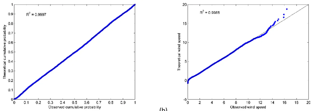
3.4 Assessment of goodness-of-fit

12

To evaluate the goodness-of-fit of the pdfs to the wind speed data, the ln L, two variants of the 230

2

R , the 2 and the KS were used. A number of approaches to compute the 2

R statistic are 231

found in the literature and are considered in this study. Thus, two variants of 2

R are computed: 232

2

PP

R which uses the P-P probability plot approach and R_QQ2 which uses the Q-Q probability plot 233

approach. These indices are described in more detail in the following subsections. 234

3.4.1 log-likelihood (ln L)

235

ln L measures the goodness-of-fit of a model to a data sample. For a given pdf f_ˆ( )x with 236

distribution parameter estimates



ˆ

237





lnL ln



238

where v is the i_i th observed wind speed and n is the number of observations in the data set. A 239

higher value of this criterion indicates a better fit of the model to the data. It should be noted that 240

ln L cannot always be calculated for the LP3 and KAP distributions. The reason is that it 241

occasionally happens that at least one wind speed observation is outside the domain defined by 242

the distribution for the parameters estimated by the given estimation method. Then, at least one 243

probability density of zero is obtained which makes the calculation of the log-likelihood 244 impossible. 245 3.4.2 2 PP R 246

13 2

PP

R is the coefficient of determination associated with the P-P probability plot which plots the 247

theoretical cdf versus the empirical cumulative probabilities. R_PP2 quantifies the linear relation 248

between predicted and observed probabilities. It is computed as follows: 249 2 2 1 2 1 ˆ ( ) 1 ( ) n i i i PP n i i F F R F F      





where Fˆ_i is the predicted cumulative probability of the ith observation obtained with the 251

theoretical cdf, F is the empirical probability of the i_i th observation and

1 1 n i i F F n  



empirical probabilities are obtained with the Cunnane (1978) formula: 253 0.4 0.2 i i F n    (10) 254

where i 1,...,n is the rank for ascending ordered observations. An example of a P-P plot is 255

presented in Figure 2a for KAP/LM at the station of East of Jebel Haffet. 256 3.4.3 2 QQ R 257 2 QQ

R is the coefficient of determination associated with the Q-Q probability plot defined by the 258

predicted wind speed quantiles obtained with the inverse function of the theoretical cdf versus 259

the observed wind speed data. Plotting positions for estimated quantiles are given by the 260

empirical probabilities F defined previously. _i R_QQ2 quantifies the linear relation between 261

predicted and observed wind speeds and is computed as follows: 262

14 2 2 1 2 1 ˆ ( ) 1 ( ) n i i i QQ n i i v v R v v      





where

v

ˆ



F

( )

F

264

ith observed wind speed and

1 1 n i i v v n 





for KAP/LM at the station of East of Jebel Haffet. 266

3.4.4 Chi-square test (2 )

267

The Chi-square goodness-of-fit test judges the adequacy of a given theoretical distribution to a 268

data sample. The sample is arranged in a frequency histogram having N bins. The Chi-square test 269

statistic is given by: 270







where Oi is the observed frequency in the ith class interval and Ei is the expected frequency in the 272

ith class interval. Ei is given by F v( )i F v( i1) where vi1 and v are the lower and upper limits i

273

of the ith class interval. The size of class intervals chosen in this study is 1 m/s. A minimum 274

expected frequency of 5 is required for each bin. When an expected frequency of a class interval 275

is too small, it is combined with the adjacent class interval. This is a usual procedure as a class 276

interval with an expected frequency that is too small will have too much weight. 277

3.4.5 Kolmogorov-Smirnov (KS)

278

The KS test computes the largest difference between the cumulative distribution function of the 279

model and the empirical distribution function. The KS test statistic is given by: 280

15 1 ˆ max _{i i} i n D F F     (13) 281

where Fˆ_i is the predicted cumulative probability of the ith observation obtained with the 282

theoretical cdf and F is the empirical probability of the i_i th observation obtained with Eq. (10). 283

284

4 Results

285

Each selected pdf was fitted to the wind speed series with the different methods and the statistics 286

of goodness-of-fit were afterwards calculated. The results are presented here separately for 287

stations with an anemometer at the 10 m height and for stations with anemometers at other 288

heights. 289

4.1 Description of wind speed data

290

Table 3 presents the descriptive statistics of each station including maximum, mean, median, 291

standard deviation, coefficient of variation, coefficient of skewness and coefficient of kurtosis. 292

For stations at 10 m, mean wind speeds vary from 2.47 m/s to 4.28 m/s. The coefficients of 293

variation are moderately low, ranging from 0.46 to 0.7. All coefficients of skewness are positive, 294

indicating that all distributions are right skewed. The coefficients of kurtosis are moderately 295

high, ranging from 2.9 to 4.47. 296

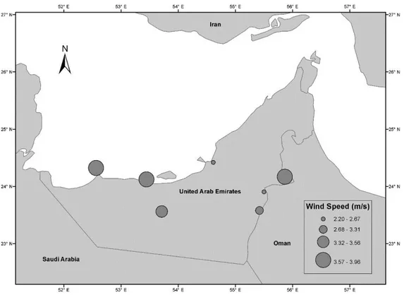
Figures 3 and 4 present respectively the spatial distribution of the median wind speed and the 297

altitude of the stations at 10 m. The circle sizes in Figures 3 and 4 are respectively proportional 298

to the median wind speeds and the altitudes of stations. Generally, coastal sites (Sir Bani Yas 299

Island, Al Mirfa and Masdar City) and sites near the mountainous region (East of Jebel Haffet) 300

16

are subject to higher mean wind speeds than inland sites. Two of the coastal sites of this study 301

have high wind speeds. However, Masdar City is characterized by lower wind speeds. 302

Altitude is an important factor to explain wind speeds. For this study, the largest median wind 303

speed occurs at East of Jebel Haffet, which is also the station that is located at the highest 304

altitude (341 m) among the 10 m height stations. However, Al Aradh, also located at a relatively 305

high altitude (178 m), has the lowest median wind speed. This shows that a diversity of other 306

factors affect wind speeds and a simple relation between mean values and geophysical 307

characteristics is difficult to establish. It is necessary to study in detail the effects of other factors 308

such as large-scale and small-scale features, terrain characteristics, presence of obstacles, surface 309

roughness, presence of ridges and ridge concavity in the dominant windward direction, and 310

channeling effect. 311

4.2 Stations at 10 m height

312

Table 4 presents the goodness-of-fit statistics for each distribution associated with a method 313

(D/M) for the stations at 10 m height. Since R , _PP2 RQQ2 ,

2

 and KS allow comparing different 314

samples together, the statistics obtained are presented with box plots in Figure 5. LN2 leading to 315

poor fits has been discarded from these box plots. Table 5 lists the 6 best D/Ms based on all 316

goodness-of-fit statistics. The best one-component parametric pdfs are denoted with superscript 317

letter a and the best two-component mixture parametric pdfs are denoted with superscript letter b 318

in Table 5. The performances of one-component parametric models are first analyzed here and 319

the comparison with mixture models and the non-parametric model is carried out afterwards. 320

The box plots of statistics in Figure 5 are used to analyze the performances of one-component 321

parametric pdfs. Based on 2

PP

R , KAP/LM leads to the best fits followed closely by GG/MM. 322

17

Based on R_QQ2 , GG/MM is the best D/M followed closely by KAP/LM. Based on 2, GG/MM 323

leads to the best fit followed closely by W3/ML. Finally, based on KS, KAP/LM is the best D/M 324

followed by GG/MM. With all statistics considered in this study, the W2 is the best 2-parameter 325

distribution and leads to better performances than the 3-parameter distributions GEV and LN3. 326

Box plots reveal also that D/Ms using MM are somewhat preferred over those that use ML. 327

Ranks of one-component parametric models in Table 5 are analyzed here. Based on ln L, 328

KAP/ML and GG/ML are the best D/Ms for 3 stations. Even if GG is often one of the best 329

ranked pdf, it is not even included among the best pdfs for the stations of Al Mirfa, East of Jebel 330

Haffet and Madinat Zayed. On the other hand, the KAP is included within the best D/Ms for all 7 331

stations. It is important also to notice that D/Ms using ML, a method that maximizes the log-332

likelihood function, are preferred by ln L over D/Ms using other methods. For 2

PP

R , the 333

KAP/LM is the best D/M for 5 stations. GG, being the second best pdf, is not even among the 334

best 6 D/Ms for most stations. Based on the R_QQ2 statistic, GG/MM is the best D/M for 4 stations 335

and is ranked the overall third best for two other stations. However, GG is not listed among the 336

best D/Ms for the station of East-of-Jebel Haffet, while KAP/LM is within the best D/Ms for all 337

stations. Based on 2, GG/MM is the best D/M for 4 stations in Table 5. However, GG is not 338

within the best 6 D/Ms for East of Jebel Haffet. Based on KS, KAP/LM is the best D/M for 5 339

stations and is among the 6 best D/Ms for every station. GG, the second best pdf, is not within 340

the best 6 D/Ms for East of Jebel Haffet, Madinat Zayed and Sir Bani Yas Island. 341

Globally, the best performances for one-component parametric models are obtained with the 342

KAP and GG. For 2

PP

R and KS, KAP is clearly the preferred distribution. For ln L, R_QQ2 and 2, 343

18

either KAP or GG can be considered as the preferred distribution. However, the GG distribution 344

is less flexible. Indeed, GG is often not selected among the 6 best D/Ms. 345

Mixture distributions MWW/LS and MGG/LS are among the distributions giving the best fits 346

with respect to box plots of statistics. For instance, MWW/LS is the best overall model according 347

to 2

PP

R and KS. MWW/LS performs very well for most stations with respect to 2. However, 348

the box plot for MWW/LS reveals the presence of an outlier (Madinat Zayed) for this statistic. 349

MWW/LS gives generally better fits than MGG/LS according to every statistic. 350

Results in Table 5 show that, according to ln L, MWW/LS is not within the best 6 D/Ms for 3 351

stations. MWW/LS is ranked first for 5 stations based on 2

PP

R . Based on R_QQ2 , MWW/LS is the 352

best D/M for 3 stations but is not ranked within the best 6 D/Ms for 3 other stations. Based on 353

2

 , MWW/LS is the best parametric model for 4 stations. Based on KS, it is ranked first for 4 354

stations and is ranked second otherwise. 355

According to ln L, 2

PP

R , R_QQ2 and KS, the non-parametric model KE generally does not provide 356

improved fits compared to parametric models. However, based on 2, KE is the best distribution 357

followed closely by MWW/LS. Both pdfs are ranked first at 3 stations each. As 2 puts more 358

weight on class intervals with lower frequency, it could be hypothesized that KE models better 359

the upper tail of wind speed distributions than other pdfs. 360

Figure 6 illustrates the frequency histograms and normal probability plots of the wind speed of 361

each station. The pdfs of W2/MM, KAP/LM, MWW/LS and KE are superimposed over these 362

plots. These D/Ms are selected to represent the one-component parametric, the mixture and the 363

non-parametric models. KAP/LM is selected among one-component parametric distributions 364

19

because it has been shown to lead to the overall best performances for the 7 stations. The W2 is 365

included for comparison purposes since it is commonly accepted for wind speed modeling. It can 366

be noticed that KAP/LM shows considerably more flexibility for Masdar City and Sir Bani Yas 367

Island. The W2 is generally not suitable. For instance, it overestimates wind speed frequencies 368

for bins of median wind speed for Al Aradh and Sir Bani Yas Island and underestimates them for 369

East of Jebel Haffet and Madinat Zayed. Histograms of Al Aradh, Masdar City and Sir Bani Yas 370

Island show clearly the presence of a bimodal regime. In these cases, the more flexible models 371

MWW/LS and KE show a clear advantage. MWW/LS is the most flexible distribution and it is 372

particularly efficient to model the histograms of Masdar City and Sir Bani Yas Island. For a 373

station presenting a strong unimodal regime, like Al Mirfa, the fits given by the different models 374

are all similar. 375

4.3 Stations at different heights

376

Table 6 presents the goodness-of-fit statistics obtained with each D/M at each height for the 377

station of Al Hala and the Masdar Wind Station. The values of the statistics are presented with 378

box plots in Figures 7 and 8 for the station of Al Hala and the Masdar Wind Station respectively. 379

Tables 7 and 8 list the 6 best D/Ms based on every statistic for each station respectively. 380

Performances of one-component parametric models are first evaluated. Box plots reveal that for 381

Al Hala, very good fits and small variances of the statistics are obtained for the majority of 382

distributions. The small variance indicates a slight variation of the wind speed distribution 383

between the heights of 40 m and 80 m. The W2 is one of the distributions giving the best 384

statistics. For the Masdar Wind Station, the variance of the various statistics is higher. KAP/LM 385

is by far the best D/M for every statistic. 386

20

Analysis of Table 7 reveals that, for the Al Hala station, W3/ML followed by GG/ML are the 387

best D/Ms at every height according to ln L. P3/MM is the best D/M at 40 m and 60 m height, 388

and W2/ML is the best D/M at 80 m based on 2

PP

R . GG/MM followed by GG/ML and W3/ML 389

give the best fits with respect to R_QQ2 . GG/ML at 40 m and 60 m, and W3/ML at 80 m give the 390

best fit with respect to 2. P3/MM is the best D/M at 40 m and 80 m, and LN3/MM is the best 391

D/M at 60 m based on KS. For the Masdar Wind Station, analysis of Table 8 reveals that KAP 392

generally represents the best parametric distribution. KAP/ML is the best D/M at three heights 393

according to ln L. KAP/LM is the best D/M at every height based on 2

PP

R and KS, and at three 394

heights based on 2. Based on R_QQ2 , KAP/LM is ranked first at the 10 m and 30 m, and 395

KAP/ML is ranked first at the 40 m heights. 396

Box plots reveal that mixture models give the overall best fits at both stations. MWW/LS is 397

generally better than MGG/LS. The variance of the boxplots of R_QQ2 for MGG is very high for 398

Al Hala. It is caused by a less accurate fit only at 40 m. Mixture models are superior to KE. In 399

the case of Al Hala, the improvement obtained with mixture models is not very high. For Masdar 400

Wind Station, a flexible model, such as a mixture model, is required. KAP is the only one-401

component parametric distribution which can model the data. 402

Figures 9 and 10 present frequency histograms and normal probability plots of wind speed for 403

each height at the station of Al Hala and the Masdar Wind Station respectively. The pdfs of 404

W2/MM, KAP/LM, MWW/LS and KE are superimposed in these plots. Histogram shapes show 405

that all the empirical distributions at Al Hala are unimodal and do not change with height. This 406

explains the small variance in statistics. For Al Hala station, each selected D/M gives 407

21

approximately the same fit for all 3 heights. Relatively little change is observed from one height 408

to another. In that case, flexible models do not provide any advantages. For the Masdar Wind 409

Station, bimodal shapes are observed at lower heights and become unimodal at higher heights. At 410

lower altitudes, the more flexible model MWW/LS and KE clearly show an advantage while at 411

50 m, all models provide equivalent fits. 412

5 Conclusions

413

The W2 distribution has been frequently suggested for the characterization of short term wind 414

speed data in a large number of regions in the world. In this study, 11 one-component pdfs, 2 415

two-component mixture pdfs and the kernel density pdf were fitted to hourly average wind speed 416

series from 9 meteorological stations located in the UAE. This region is characterized by a 417

severe lack of studies focusing on the assessment of wind speed characteristics and distributions. 418

For each pdf, one or more estimation methods were used to estimate the parameters of the 419

distribution. Different goodness-of-fit measurements have been used to evaluate the suitability of 420

pdfs over wind speed data. 421

Overall, mixture distributions are generally the best pdfs according to every statistic. MWW is 422

more suitable than MGG most of the time. The non-parametric KE method does not generally 423

lead to best performances. Results show also clearly that one-component pdfs are not suitable for 424

modeling distributions presenting bimodal regimes. In this case, mixture distributions should be 425

employed. 426

Overall, and for all stations and heights, the best one-component pdfs are KAP and GG. W2 is 427

the best 2-parameter distribution and performs better than some 3-parameter distributions such as 428

the GEV and LN3. 429

22

Acknowledgements

430

The financial support provided by the Masdar Institute of Science and Technology is gratefully 431

acknowledged. The authors wish to thank Masdar Power for having supplied the wind speed data 432

used in this study. 433

23

Nomenclature

cdf cumulative distribution function 439

2

 Chi-square test statistic 440

D/M distribution/method 441

EV1 Gumbel or extreme value type I distribution 442

ˆ( )

f_ probability density function with estimated parameters ˆ 443

ˆ( )

f estimated probability density function 444

i

F empirical probability for the ith wind speed observation 445

ˆ

i

F estimated cumulative probability for the ith observation obtained with the theoretical cdf 446

( )

F cumulative distribution function 447

1

( )

F inverse of a given cumulative distribution function 448

G Gamma distribution 449

GEV generalized extreme value distribution 450

GG generalized Gamma distribution 451

GMM generalized method of moment 452

K( ) kernel function 453

KAP Kappa distribution 454

24 KE Kernel density distribution

455

KS Kolmogorov-Smirnov test statistic 456

LN2 2-parameter Lognormal distribution 457

LN3 3-parameter Lognormal distribution 458

MGG mixture of two Gamma pdfs 459

ML maximum likelihood 460

MM method of moments 461

MWW mixture of two 2-parameter Weibull pdfs 462

n number of wind speed observations in a series of wind speed observations 463

N number of bins in a histogram of wind speed data 464

P3 Pearson type III distribution 465

pdf probability density function 466 2 R coefficient of determination 467 2 PP

R coefficient of determination giving the degree of fit between the theoretical cdf and the 468

empirical cumulative probabilities of wind speed data. 469

2

QQ

R coefficient of determination giving the degree of fit between the theoretical wind speed 470

quantiles and the wind speed data. 471

RAY Rayleigh distribution 472

rmse root mean square error 473

i

v the ith observation of the wind speed series 474

ˆ_i

v predicted wind speed for the ith observation 475

25 W2 2-parameter Weibull distribution

476

W3 3-parameter Weibull distribution 477

WMM weighted method of moments 478

479 480

26

References

481

Acker, T.L., Williams, S.K., Duque, E.P.N., Brummels, G., Buechler, J., 2007. Wind resource 482

assessment in the state of Arizona: Inventory, capacity factor, and cost. Renewable Energy 483

32(9), 1453-1466. 484

Ahmed Shata, A.S., Hanitsch, R., 2006. Evaluation of wind energy potential and electricity 485

generation on the coast of Mediterranean Sea in Egypt. Renewable Energy 31(8), 1183-486

1202. 487

Akpinar, E.K., Akpinar, S., 2005. A statistical analysis of wind speed data used in installation of 488

wind energy conversion systems. Energy Conversion and Management 46(4), 515-532. 489

Akpinar, S., Kavak Akpinar, E., 2007. Wind energy analysis based on maximum entropy 490

principle (MEP)-type distribution function. Energy Conversion and Management 48(4), 491

1140-1149. 492

Akpinar, S., Akpinar, E.K., 2009. Estimation of wind energy potential using finite mixture 493

distribution models. Energy Conversion and Management 50(4), 877-884. 494

Algifri, A.H., 1998. Wind energy potential in Aden-Yemen. Renewable Energy 13(2), 255-260. 495

Archer, C.L., Jacobson, M.Z., 2003. Spatial and temporal distributions of U.S. winds and wind 496

power at 80 m derived from measurements. Journal of Geophysical Research: 497

Atmospheres 108(D9), 4289. 498

Ashkar, F., Ouarda, T.B.M.J., 1996. On some methods of fitting the generalized Pareto 499

distribution. Journal of Hydrology 177(1–2), 117-141. 500

Auwera, L., Meyer, F., Malet, L., 1980. The use of the Weibull three-parameter model for 501

estimating mean power densities. Journal of Applied Meteorology 19, 819-825. 502

27

Ayodele, T.R., Jimoh, A.A., Munda, J.L., Agee, J.T., 2012. Wind distribution and capacity 503

factor estimation for wind turbines in the coastal region of South Africa. Energy 504

Conversion and Management 64(0), 614-625. 505

Bobée, B., 1975. The Log Pearson Type 3 distribution and its application in hydrology. Water 506

Resources Research 11(5), 681-689. 507

Bobée, B., Ashkar, F., 1988. Sundry averages method (SAM) for estimating parameters of the 508

Log-Pearson Type 3 distribution. Research Report No. 251, INRS-ETE, Quebec City, 509

Canada. 510

Carta, J.A., Ramírez, P., 2007. Use of finite mixture distribution models in the analysis of wind 511

energy in the Canarian Archipelago. Energy Conversion and Management 48(1), 281-291. 512

Carta, J.A., Ramirez, P., Velazquez, S., 2008. Influence of the level of fit of a density probability 513

function to wind-speed data on the WECS mean power output estimation. Energy 514

Conversion and Management 49(10), 2647-2655. 515

Carta, J.A., Ramirez, P., Velazquez, S., 2009. A review of wind speed probability distributions 516

used in wind energy analysis Case studies in the Canary Islands. Renewable & Sustainable 517

Energy Reviews 13(5), 933-955. 518

Celik, A.N., 2003. Energy output estimation for small-scale wind power generators using 519

Weibull-representative wind data. Journal of Wind Engineering and Industrial 520

Aerodynamics 91(5), 693-707. 521

Celik, A.N., 2004. On the distributional parameters used in assessment of the suitability of wind 522

speed probability density functions. Energy Conversion and Management 45(11-12), 523

1735-1747. 524

28

Chang, T.P., 2011. Estimation of wind energy potential using different probability density 525

functions. Applied Energy 88(5), 1848-1856. 526

Chellali, F., Khellaf, A., Belouchrani, A., Khanniche, R., 2012. A comparison between wind 527

speed distributions derived from the maximum entropy principle and Weibull distribution. 528

Case of study; six regions of Algeria. Renewable & Sustainable Energy Reviews 16(1), 529

379-385. 530

Conradsen, K., Nielsen, L.B., Prahm, L.P., 1984. Review of Weibull Statistics for Estimation of 531

Wind Speed Distributions. Journal of Climate and Applied Meteorology 23(8), 1173-1183. 532

Cunnane, C., 1978. Unbiased plotting positions — A review. Journal of Hydrology 37(3–4), 533

205-222. 534

Dorvlo, A.S.S., 2002. Estimating wind speed distribution. Energy Conversion and Management 535

43(17), 2311-2318. 536

Fichaux, N., Ranchin, T., 2003. Evaluating the offshore wind potential. A combined approach 537

using remote sensing and statistical methods. In: Proceedings IGARSS'03 - IEEE 538

International Geoscience and Remote Sensing Symposium, Toulouse, France, Vol. 4, pp. 539

2703-2705. 540

Garcia, A., Torres, J.L., Prieto, E., De Francisco, A., 1998. Fitting wind speed distributions: A 541

case study. Solar Energy 62(2), 139-144. 542

Gökçek, M., Bayülken, A., Bekdemir, Ş., 2007. Investigation of wind characteristics and wind 543

energy potential in Kirklareli, Turkey. Renewable Energy 32(10), 1739-1752. 544

Guidoum, A.C., 2014. kedd: Kernel estimator and bandwidth selection for density and its 545

derivatives. R package version 1.0.1. URL http://CRAN.R-project.org/package=kedd 546

29

Hennessey, J.P., 1977. Some aspects of wind power statistics. Journal of Applied Meteorology 547

16(2), 119-128. 548

Hosking, J.R.M., Wallis, J.R., 1997. Regional Frequency Analysis: An Approach Based on L-549

Moments. Cambridge University Press. 550

Hosking J.R.M., 1996. Fortran routines for use with the method of L-moments, version 3.04. 551

Research report 20525, IBM Research Division. 552

Hundecha, Y., St-Hilaire, A., Ouarda, T.B.M.J., El Adlouni, S., Gachon, P., 2008. A 553

Nonstationary Extreme Value Analysis for the Assessment of Changes in Extreme Annual 554

Wind Speed over the Gulf of St. Lawrence, Canada. Journal of Applied Meteorology and 555

Climatology 47(11), 2745-2759. 556

Irwanto, M., Gomesh, N., Mamat, M.R., Yusoff, Y.M., 2014. Assessment of wind power 557

generation potential in Perlis, Malaysia. Renewable and Sustainable Energy Reviews 558

38(0), 296-308. 559

Jaramillo, O.A., Saldaña, R., Miranda, U., 2004. Wind power potential of Baja California Sur, 560

México. Renewable Energy 29(13), 2087-2100. 561

Jones, M.C., Marron, J.S., Sheather, S.J., 1996. A brief survey of bandwidth selection for 562

density estimation. Journal of the American Statistical Association 91(433), 401-407. 563

Justus, C.G., Hargraves, W.R., Mikhail, A., Graber, D., 1978. Methods for Estimating Wind 564

Speed Frequency Distributions. Journal of Applied Meteorology 17(3), 350-353. 565

Justus, C.G., Hargraves, W.R., Yalcin, A., 1976. Nationwide assessment of potential output 566

from wind-powered generators. Journal of Applied Meteorology 15(7), 673-678. 567

Kose, R., Ozgur, M.A., Erbas, O., Tugcu, A., 2004. The analysis of wind data and wind energy 568

potential in Kutahya, Turkey. Renewable and Sustainable Energy Reviews 8(3), 277-288. 569

30

Li, M., Li, X., 2005. MEP-type distribution function: a better alternative to Weibull function for 570

wind speed distributions. Renewable Energy 30(8), 1221-1240. 571

Lo Brano, V., Orioli, A., Ciulla, G., Culotta, S., 2011. Quality of wind speed fitting distributions 572

for the urban area of Palermo, Italy. Renewable Energy 36(3), 1026-1039. 573

Masseran, N., Razali, A.M., Ibrahim, K., 2012. An analysis of wind power density derived from 574

several wind speed density functions: The regional assessment on wind power in 575

Malaysia. Renewable & Sustainable Energy Reviews 16(8), 6476-6487. 576

Mirhosseini, M., Sharifi, F., Sedaghat, A., 2011. Assessing the wind energy potential locations 577

in province of Semnan in Iran. Renewable and Sustainable Energy Reviews 15(1), 449-578

459. 579

Morgan, E.C., Lackner, M., Vogel, R.M., Baise, L.G., 2011. Probability distributions for 580

offshore wind speeds. Energy Conversion and Management 52(1), 15-26. 581

Nfaoui, H., Buret, J., Sayigh, A.A.M., 1998. Wind characteristics and wind energy potential in 582

Morocco. Solar Energy 63(1), 51-60. 583

Ordóñez, G., Osma, G., Vergara, P., Rey, J., 2014. Wind and Solar Energy Potential Assessment 584

for Development of Renewables Energies Applications in Bucaramanga, Colombia. IOP 585

Conference Series: Materials Science and Engineering 59(1), 012004. 586

Ouarda, T.B.M.J., Charron, C., Niranjan Kumar, K., Marpu, P.R., Ghedira, H., Molini, A., 587

Khayal, I., 2014. Evolution of the rainfall regime in the United Arab Emirates. Journal of 588

Hydrology 514(0), 258-270. 589

Persaud, S., Flynn, D., Fox, B., 1999. Potential for wind generation on the Guyana coastlands. 590

Renewable Energy 18(2), 175-189. 591

31

Petković, D., Shamshirband, S., Anuar, N.B., Saboohi, H., Abdul Wahab, A.W., Protić, M., 592

Zalnezhad, E., Mirhashemi, S.M.A., 2014. An appraisal of wind speed distribution 593

prediction by soft computing methodologies: A comparative study. Energy Conversion 594

and Management 84(0), 133-139. 595

Poje, D., Cividini, B., 1988. Assessment of wind energy potential in croatia. Solar Energy 41(6), 596

543-554. 597

Qin, Z.L., Li, W.Y., Xiong, X.F., 2011. Estimating wind speed probability distribution using 598

kernel density method. Electric Power Systems Research 81(12), 2139-2146. 599

Qin, X., Zhang, J.-s., Yan, X.-d., 2012. Two Improved Mixture Weibull Models for the Analysis 600

of Wind Speed Data. Journal of Applied Meteorology and Climatology 51(7), 1321-1332. 601

Ramirez, P., Carta, J.A., 2006. The use of wind probability distributions derived from the 602

maximum entropy principle in the analysis of wind energy. A case study. Energy 603

Conversion and Management 47(15-16), 2564-2577. 604

Şahin, A.Z., Aksakal, A., 1998. Wind power energy potential at the northeastern region of Saudi 605

Arabia. Renewable Energy 14(1–4), 435-440. 606

Seguro, J.V., Lambert, T.W., 2000. Modern estimation of the parameters of the Weibull wind 607

speed distribution for wind energy analysis. Journal of Wind Engineering and Industrial 608

Aerodynamics 85(1), 75-84. 609

Singh, V., Deng, Z., 2003. Entropy-Based Parameter Estimation for Kappa Distribution. Journal 610

of Hydrologic Engineering 8(2), 81-92. 611

Soukissian, T., 2013. Use of multi-parameter distributions for offshore wind speed modeling: 612

The Johnson SB distribution. Applied Energy 111(0), 982-1000. 613

32

Stewart, D.A., Essenwanger, O.M., 1978. Frequency Distribution of Wind Speed Near the 614

Surface. Journal of Applied Meteorology 17(11), 1633-1642. 615

Sulaiman, M.Y., Akaak, A.M., Wahab, M.A., Zakaria, A., Sulaiman, Z.A., Suradi, J., 2002. 616

Wind characteristics of Oman. Energy 27(1), 35-46. 617

Takle, E.S., Brown, J.M., 1978. Note on use of Weibull statistics to characterize wind speed 618

data. Journal of Applied Meteorology 17(4), 556-559. 619

Tuller, S.E., Brett, A.C., 1985. The goodness of fit of the Weilbull and Rayleigh distribution to 620

the distributions of observed wind speeds in a topographically diverse area. Journal of 621

climatology 5, 74-94. 622

Ulgen, K., Hepbasli, A., 2002. Determination of Weibull parameters for wind energy analysis of 623

Izmir, Turkey. International Journal of Energy Research 26(6), 495-506. 624

Usta, I., Kantar, Y.M., 2012. Analysis of some flexible families of distributions for estimation of 625

wind speed distributions. Applied Energy 89(1), 355-367. 626

Water Resources Council, Hydrology Committee, 1967. A uniform technique for determining 627

flood flow frequencies. US Water Resour. Counc., Bull. No. 15, Washington, D.C. 628

Zhang, H., Yu, Y.-J., Liu, Z.-Y., 2014. Study on the Maximum Entropy Principle applied to the 629

annual wind speed probability distribution: A case study for observations of intertidal zone 630

anemometer towers of Rudong in East China Sea. Applied Energy 114(0), 931-938. 631

Zhang, J., Chowdhury, S., Messac, A., Castillo, L., 2013. A Multivariate and Multimodal Wind 632

Distribution model. Renewable Energy 51(0), 436-447. 633

Zhou, J.Y., Erdem, E., Li, G., Shi, J., 2010. Comprehensive evaluation of wind speed 634

distribution models: A case study for North Dakota sites. Energy Conversion and 635

Management 51(7), 1449-1458. 636

33 Table 1. Description of the meteorological stations. 637

Station Measuring Height (m)

Altitude

(m) Latitude Longitude Period (year/month)

Al Aradh 10 178 23.903° N 55.499° E 2007/06 - 2010/08

Al Mirfa 10 6 24.122° N 53.443° E 2007/06 - 2009/07

Al Wagan 10 142 23.579° N 55.419° E 2009/08 - 2010/08

East of Jebel Haffet 10 341 24.168° N 55.864° E 2009/10 - 2010/08 Madinat Zayed 10 137 23.561° N 53.709° E 2008/06 - 2010/08

Masdar City 10 7 24.420° N 54.613° E 2008/07 - 2010/08

Sir Bani Yas Island 10 7 24.322° N 52.566° E 2007/06 - 2010/08 Al Hala 40, 60, 80 N/A 25.497° N 56.143° E 2009/08 - 2010/08 Masdar Wind Station 10, 30, 40, 50 0.6 24.420° N 54.613° E 2008/08 - 2011/02

638

639 640

34

Table 2. List of probability density functions, domain, number of parameters and estimation methods 641

used. 642

Name pdf Domain Number of

parameters

Estimation method

EV1 f x  1exp x  exp x 

         _  _{ }        x 2 ML, MM W2   1 exp k k k x x f x     _{ }       _{ }  _{ }      x 0 2 ML, MM G   _{ } 1exp( ) k k f x x x k   _    x 0 2 ML, MM LN2     2 2 ln 1 exp 2 2 x f x x               x 0 2 ML, MM W3   1 exp k k k x x f x       _{ }        _ _ __ _ _   x _{3 ML} LN3   _{ }   2 2 ln 1 exp 2 2 x m f x x m      _{   }          _ _ xm 3 ML, MM GEV       1 1 1/ 1 1 exp 1 k k k k f x x u x u     _{ }        _   _ _ _  _ _   / if 0 / if 0 x u k k x u k k         3 ML, MM GG   _{ } 1_{exp( )} hk hk h h f x x x k   _    x 0 3 ML, MM P3   _{ }  1exp   k k f x x x k  _  _{ }   _  _  x _{3 ML, MM} LP3         1

loga k exp loga g f x x x x k        _  _ _  _  loga g e /g /g if 0 0 if 0 x e x e          3 GMM KAP 1 1/ 1 1 ( ) [1 ( ) / ]k [ ( )]h f x  k x   F x  where _{F x( ) (1 h(1k x( } _{) / ) )}1/k1/h / if 0 (1 ) / if 0 / if 0, 0 k x k k h k x k k x h k                   4 LM, ML MWW   11 1 21 2 1 2 1 1 1 2 2 2 exp (1 ) exp k k k k k x x k x x f x          _{ }  _{ }   _   _   _   _                  _   _   _   _ 0 x 5 LS MGG   _{   } 2 1 11 2 21 1 2 1 2 exp( ) (1 ) exp( ) k k k k f x x x x x k k                x0 5 LS μ: location parameter. 643

m: second location parameter (LN3). 644

α: scale parameter. 645

k: shape parameter. 646

h: second shape parameter (GG, KAP). 647

ω: mixture parameter (MWW, MGG). 648

Γ( ): gamma function. 649

35

Table 3. Descriptive statistics of wind speed series. Maximum, mean, median, standard deviation (SD), 650

coefficient of variation (CV), coefficient of skewness (CS) and coefficient of kurtosis (CK).

651 Station Height (m) Maximum (m/s) Mean (m/s) Median (m/s) SD (m/s) CV CS CK Al Aradh 10 12.42 2.47 2.20 1.73 0.70 0.97 4.20 Al Mirfa 10 17.17 4.28 3.96 2.26 0.53 0.71 3.58 Al Wagan 10 12.36 3.67 3.31 2.22 0.61 0.66 3.08

East of Jebel Haffet 10 16.41 4.27 3.87 2.35 0.55 0.99 4.47

Madinat Zayed 10 18.04 4.10 3.56 2.44 0.60 0.94 3.83

Masdar City 10 12.17 3.09 2.67 2.06 0.67 0.70 2.90

Sir Bani Yas Island 10 13.95 3.86 3.76 2.14 0.55 0.43 3.06

Al Hala 40 16.42 5.61 5.43 2.66 0.47 0.58 3.29

60 16.72 5.67 5.50 2.72 0.48 0.56 3.27

80 16.67 5.80 5.63 2.68 0.46 0.54 3.25

Masdar Wind Station 10 13.02 3.16 2.69 1.87 0.59 0.82 3.09

30 15.20 3.85 3.44 2.01 0.52 0.80 3.37 40 15.73 4.06 3.71 2.02 0.50 0.76 3.43 50 16.26 4.37 4.05 2.13 0.49 0.77 3.73 652 653 654

36

Table 4. Statistics obtained with each D/M for the stations at 10 m height. 655

Statistic D/M Al Aradh Al Mirfa Al Wagan

East of Jebel Haffet Madinat Zayed Masdar City Sir Bani Yas Island ln L EV1/ML -51761 -40610 -13777 -14608 -39966 -37939 -58656 EV1/MM -51763 -40685 -13789 -14610 -39968 -37943 -59097 W2/ML -50928 -40561 -13664 -14664 -40032 -37156 -58726 W2/MM -51070 -40564 -13670 -14664 -40034 -37172 -58873 W3/ML -50717 -40468 -13622 -14654 -39916 -37130 -57870 LN2/ML -57510 -43750 -14901 -15502 -43435 -39738 -67410 LN2/MM -74925 -47170 -16939 -16309 -47573 -44668 -87395 G/ML -51519 -41044 -13841 -14745 -40339 -37452 -60260 G/MM -52696 -41280 -13995 -14781 -40502 -37767 -62402 GEV/ML -51730 -40551 -13773 -14608 -39954 -37914 -58239 GEV/MM -51854 -40561 -13794 -14610 -40038 -38121 -58246 LN3/ML -51537 -40538 -13752 -14605 -39911 -37709 -58250 LN3/MM -51813 -40573 -13810 -14608 -40041 -38185 -58278 GG/ML -50349 -40554 -13608 -14658 -40032 -37017 -57778 GG/MM -50556 -40596 -13610 -14709 -40081 -37031 -57902 P3/ML -51084 -40492 -13694 -14605 -39861 -37340 -58196 P3/MM -51535 -40523 -13783 -14615 -39923 -38073 -58249 LP3/GMM x x -13706 -14831 -40493 x x KAP/ML -50738 -40477 -13614 -14603 -39847 -36999 -58063 KAP/LM -51251 -40491 -13623 -14604 -39905 x x MWW/LS -50520 -40570 -13633 -14616 -40263 -36979 -57288 MGG/LS -50228 -40921 -13702 -14772 -40587 -37182 -58114 KE -51754 -40623 -13815 -14697 -40027 -37544 -58080 2 PP R EV1/ML 0.9972 0.9986 0.9958 0.9998 0.9977 0.9871 0.9917 EV1/MM 0.9976 0.9962 0.9926 0.9997 0.9975 0.9855 0.9858 W2/ML 0.9922 0.9994 0.9984 0.9962 0.9962 0.9960 0.9869 W2/MM 0.9970 0.9996 0.9985 0.9963 0.9962 0.9943 0.9947 W3/ML 0.9968 0.9994 0.9990 0.9960 0.9956 0.9957 0.9980 LN2/ML 0.9167 0.9640 0.9538 0.9707 0.9619 0.9709 0.8844 LN2/MM 0.9636 0.9843 0.9695 0.9930 0.9911 0.9526 0.9600 G/ML 0.9793 0.9939 0.9908 0.9956 0.9957 0.9936 0.9594 G/MM 0.9919 0.9975 0.9927 0.9994 0.9991 0.9872 0.9841 GEV/ML 0.9967 0.9990 0.9956 0.9997 0.9985 0.9885 0.9984 GEV/MM 0.9984 0.9991 0.9961 0.9995 0.9964 0.9877 0.9989 LN3/ML 0.9964 0.9991 0.9963 0.9997 0.9989 0.9909 0.9982 LN3/MM 0.9986 0.9989 0.9955 0.9994 0.9961 0.9868 0.9991 GG/ML 0.9965 0.9992 0.9992 0.9973 0.9960 0.9966 0.9935 GG/MM 0.9985 0.9998 0.9993 0.9992 0.9977 0.9971 0.9981 P3/ML 0.9942 0.9995 0.9973 0.9993 0.9986 0.9943 0.9977 P3/MM 0.9993 0.9994 0.9964 0.9994 0.9973 0.9885 0.9991 LP3/GMM 0.9961 0.9995 0.9995 0.9989 0.9984 0.9988 0.9954 KAP/ML 0.9938 0.9998 0.9995 0.9996 0.9984 0.9982 0.9960 KAP/LM 0.9994 0.9998 0.9996 0.9997 0.9989 0.9992 0.9993 MWW/LS 0.9994 0.9997 0.9998 0.9999 0.9993 0.9999 0.9999 MGG/LS 0.9999 0.9997 0.9992 0.9997 0.9992 0.9991 0.9996 KE 0.9988 0.9988 0.9973 0.9963 0.9978 0.9978 0.9993 2 QQ R EV1/ML 0.9943 0.9867 0.9813 0.9975 0.9930 0.9750 0.9569 EV1/MM 0.9945 0.9907 0.9833 0.9978 0.9931 0.9753 0.9746 W2/ML 0.9880 0.9990 0.9944 0.9936 0.9972 0.9854 0.9827 W2/MM 0.9974 0.9991 0.9966 0.9935 0.9971 0.9886 0.9936