Embedded and validated control algorithms for the spacecraft rendezvous

THÈSE

DOCTORAT DE L’UNIVERSITÉ FÉDÉRALE TOULOUSE

MIDI-PYRÉNÉES

Délivré par :

l’Université Toulouse 3 Paul Sabatier (UT3 Paul Sabatier)

Présentée et soutenue le 17/10/2018 par :

Paulo Ricardo ARANTES GILZ

Embedded and validated control algorithms for the spacecraft rendezvous

JURY

M. Luca ZACCARIAN LAAS-CNRS Président du Jury

M. Alejandro Hernán GONZÁLEZ INTEC / CONICET / UNL Rapporteur

M. Eric KERRIGAN Imperial College London Rapporteur

Mme Estelle COURTIAL Université d’Orléans / PRISME Examinateur

Mme Gabriella GAIAS DLR München Examinateur

M. Massimiliano VASILE University of Strathclyde Examinateur

M. Frédéric CAMPS LAAS-CNRS Membre invité

École doctorale et spécialité :

MITT : Domaine Mathématiques : Mathématiques appliquées Unité de Recherche :

Laboratoire d’analyse et d’architecture des systèmes Directeur(s) de Thèse :

Mme Mioara JOLDEŞ et M. Christophe LOUEMBET Rapporteurs :

Infinitely many thanks to Mioara Joldeş and Christophe Louembet for enlightening my path during this three-years-long journey. I will never be able to show you how much I am thankful for your advices and collaboration.

A special thanks to Frédéric Camps, whose help and dedication were essential for the accomplishment and quality of the produced work.

Thanks to all the members of the Methods and Algorithms in Control group of the LASS-CNRS for hosting me and for supporting me in this project.

I would also like to thank my coworkers from INSA Toulouse, Saïd Zabi, Pierre Dauchez, Audine Subias and Vincent Mahout, for all the moments together and for everything they taught me.

Huge thanks to all the PhD students and interns that I had the pleasure to meet and with whom I could share my joys and sorrows all along these years. You did made it much more enjoyable this way. ¡Sofia, gracias por la ayuda, consejos y conversaciones, sis!

Obrigado a minha mãe, meu pai e minha irmã. Tirei de vocês a oportunidade de estarmos juntos durante três longos anos. Serei sempre grato pelo carinho e preocupação de vocês. Obrigado também a meus avós Zofia e Viktor. Só pude chegar onde cheguei pela ajuda de vocês, mas infelizmente vocês partiram antes de poder ver. Esta tese é para vocês.

Funding Sources

This PhD thesis was supported by the FastRelax (ANR-14-CE25-0018-01) project of the French National Agency for Research (ANR).

Autonomy is one of the major concerns during the planning of a space mission, whether its objective is scientific (interplanetary exploration, observations, etc.) or commercial (service in orbit). For space rendezvous, this autonomy depends on the on-board capacity of controlling the relative movement between two spacecraft. In the context of satellite servicing (trou-bleshooting, propellant refueling, orbit correction, end-of-life deorbit, etc.), the feasibility of such missions is also strongly linked to the ability of the guidance and control algorithms to account for all operational constraints (for example, thruster saturation or restrictions on the relative positioning between the vehicles) while maximizing the life of the vehicle (minimizing propellant consumption). The literature shows that this problem has been intensively studied since the early 2000s. However, the proposed algorithms are not entirely satisfactory. Some approaches, for example, degrade the constraints in order to be able to base the control algorithm on an efficient optimization problem. Other methods accounting for the whole set of constraints of the problem are too cumbersome to be embedded on real computers existing in the spaceships.

The main object of this thesis is the development of new efficient and validated algorithms for the impulsive guidance and control of spacecraft in the context of the so-called "hovering" phases of the orbital rendezvous, i.e. the stages in which a secondary vessel must maintain its position within a bounded area of space relatively to another main vessel. The first contribution presented in this manuscript uses a new mathematical formulation of the space constraints for the relative motion between spacecraft for the design of control algorithms with more efficient computational processing compared to traditional approaches. The second and main contribution is a predictive control strategy that has been formally demonstrated to ensure the convergence of relative trajectories towards the "hovering" zone, even in the presence of disturbances or saturation of the actuators. Specific computational developments have demonstrated the embeddability of these control algorithms on a board containing a FPGA-synthesized LEON3 microprocessor certified for space flight, reproducing the performance of the devices usually used in flight. Finally, tools for rigorous approximation of functions were used to obtain validated solutions of the equations describing the linearized relative motion, allowing a simple certified propagation of the relative trajectories via polynomials and the verification of the respect of the constraints of the problem.

L’autonomie est l’une des préoccupations majeures lors du développement de missions spatiales que l’objectif soit scientifique (exploration interplanétaire, observations, etc) ou commercial (service en orbite). Pour le rendez-vous spatial, cette autonomie dépend de la capacité embarquée de contrôle du mouvement relatif entre deux véhicules spatiaux. Dans le contexte du service aux satellites (dépannage, remplissage additionnel d’ergols, correction d’orbite, désorbitation en fin de vie, etc), la faisabilité de telles missions est aussi fortement liée à la capacité des algorithmes de guidage et contrôle à prendre en compte l’ensemble des contraintes opérationnelles (par exemple, saturation des propulseurs ou restrictions sur le positionnement relatif entre les véhicules) tout en maximisant la durée de vie du véhicule (minimisation de la consommation d’ergols). La littérature montre que ce problème a été étudié intensément depuis le début des années 2000. Les algorithmes proposés ne sont pas tout à fait satisfaisants. Quelques approches, par exemple, dégradent les contraintes afin de pouvoir fonder l’algorithme de contrôle sur un problème d’optimisation efficace. D’autres méthodes, si elles prennent en compte l’ensemble du problème, se montrent trop lourdes pour être embarquées sur de véritables calculateurs existants dans les vaisseaux spatiaux.

Le principal objectif de cette thèse est le développement de nouveaux algorithmes efficaces et validés pour le guidage et le contrôle impulsif des engins spatiaux dans le contexte des phases dites de “hovering” du rendez-vous orbital, i.e. les étapes dans lesquelles un vaisseau secondaire doit maintenir sa position à l’intérieur d’une zone délimitée de l’espace relativement à un autre vaisseau principal. La première contribution présentée dans ce manuscrit utilise une nouvelle formulation mathématique des contraintes d’espace pour le mouvement relatif entre vaisseaux spatiaux pour la conception d’algorithmes de contrôle ayant un traitement calculatoire plus efficace comparativement aux approches traditionnelles. La deuxième et principale contribution est une stratégie de contrôle prédictif qui assure la convergence des trajectoires relatives vers la zone de “hovering”, même en présence de perturbations ou de sat-uration des actionneurs. Un travail spécifique de développement informatique a pu démontrer l’embarquabilité de ces algorithmes de contrôle sur une carte contenant un microprocesseur LEON3 synthétisé sur FPGA certifié pour le vol spatial, reproduisant les performances des dispositifs habituellement utilisés en vol. Finalement, des outils d’approximation rigoureuse de fonctions ont été utilisés pour l’obtention des solutions validées des équations décrivant le mouvement relatif linéarisé, permettant ainsi une propagation certifiée simple des trajectoires relatives via des polynômes et la vérification du respect des contraintes du problème.

Acknowledgments i

Abstract iii

Résumé v

Nomenclature ix

Introduction 1

1 Modeling the problem 7

1.1 Introduction. . . 7

1.2 Relative motion . . . 9

1.2.1 Simulation model. . . 9

1.2.2 Synthesis model . . . 18

1.2.3 Deaconu’s parametrization and periodic relative trajectories . . . 23

1.3 Guidance of the relative motion . . . 26

1.3.1 Space constraints: describing the hovering region . . . 27

1.3.2 Actuators and fuel consumption . . . 30

1.3.3 Optimal guidance problem formulation. . . 33

1.4 Conclusion . . . 34

2 Solving the guidance optimization problem 37 2.1 Introduction. . . 37

2.2 Hovering zone guidance methods: bibliographic review . . . 38

2.3 Proposed methods to solve the guidance problem . . . 41

2.3.1 Discretization approach . . . 42

2.3.2 Polynomial non-negativity approach . . . 44

2.3.3 Envelopes . . . 46

2.3.4 Conclusions . . . 49

2.4 Embedded algorithms . . . 50

2.4.1 Test environment . . . 50

2.4.2 Solving the LP problems. . . 50

2.4.3 Solving the SDP problems . . . 52

2.4.4 Embedding the libraries for the LP and SDP methods . . . 54

2.4.5 Solving the ENV problems . . . 54

2.5 Simulations and results . . . 55

2.6 Conclusions . . . 60

3 Model predictive control strategy 61 3.1 Introduction. . . 61

3.2 Impulsive model predictive control . . . 62

3.3 The proposed model predictive control strategy . . . 63

3.3.1 Control algorithm . . . 64

3.3.2 Proof of convergence and invariance . . . 73

3.4 Simulations and results . . . 77

3.4.1 Processor-in-the-loop. . . 77

3.4.3 Convergence definition . . . 79

3.4.4 Consumption, convergence time and running time . . . 79

3.4.5 Relative trajectories, impulses and distance to the admissible set . . . 81

3.4.6 Impact of parameters on fuel consumption. . . 81

3.5 Conclusions . . . 87

4 Validated optimal guidance problem 91 4.1 Introduction. . . 91

4.2 Rigorous approximations and Chebyshev polynomials . . . 93

4.3 The approximation method . . . 95

4.3.1 Principles of the validation method . . . 97

4.3.2 Extensions of the method . . . 99

4.4 Example: the simplified linearized Tschauner-Hempel equations . . . 100

4.4.1 Rigorous approximation of the non-polynomial coefficient . . . 101

4.4.2 Integral transform and numerical solution . . . 101

4.4.3 Validation . . . 102

4.5 Validated guidance algorithm . . . 102

4.5.1 Validated constrained relative dynamics . . . 102

4.5.2 Fuel-optimal impulsive validated guidance problem . . . 105

4.5.3 Results . . . 106

4.6 Conclusions . . . 114

Conclusion and future works 115 A Tschauner-Hempel equations 117 A.1 Nonlinear Tschauner-Hempel equations. . . 117

A.2 Linearized Tschauner-Hempel equations . . . 119

A.3 Simplified linearized Tschauner-Hempel equations. . . 121

B Univariate non-negative polynomials 123 C Envelopes and implicitization 125 C.1 Envelope definition . . . 125

C.2 Implicitization method . . . 126

D Embedding the libraries for the LP and SDP methods 129 E Non-smooth optimization methods 131 E.1 Penalty method . . . 131

E.2 Sub-gradient method . . . 132

E.3 BFGS method applied to non-smooth functions . . . 133

E.4 BFGS + sub-gradient hybrid method. . . 134

E.5 Testing the algorithms . . . 135

E.5.1 Sub-gradient method . . . 137

E.5.2 BFGS method . . . 137

E.5.3 BFGS + sub-gradient hybrid method . . . 139

∆V Vector of instantaneous velocity corrections

J Fuel consumption

µ Earth’s gravitational constant

ν True anomaly

Ω Longitude of the ascending node

ω Argument of perigee

∆V Thrusters saturation threshold

Φ, ΦD State-transition matrices

a Semi-major axis

D Deaconu’s vector of parameters

e Eccentricity

G Universal gravitational constant

i Orbit inclination

In Identity matrix of oder n

On Null matrix of oder n

X Relative state between spacecraft in the LVLH frame

LMI Linear matrix inequality

LODE Linear ordinary differential equations

LP Linear program

LTV Linear Time-Varying

LVLH Local-vertical / local-horizontal

MPC Model predictive control

RPA Rigorous polynomial approximation

SDP Semi-definite program

Spacecraft autonomy has become an important feature in the development of space missions, especially when ground operations are impracticable due to a large number of operations or an elevated communication time. Efficient embedded algorithms dedicated to autonomous decision making and maneuvering have already been used in many space projects, such as: the Soyuz and ATV automated docking systems [37, 46], which are highly sophisticated spacecraft capable of automatically docking to the International Space Station using their own propulsion and navigation systems; and the Japanese Hayabusa asteroid touchdown mission [61], during which a spacecraft was supposed to touch the surface of an asteroid with its sample capturing device and then take off again.

Indeed, mastering the implementation of efficient embedded algorithms and assessing their performance are crucial for the accomplishment of mission goals, but also open a venue of economical opportunities and allow the feasibility of future space applications. One example in the context of space exploration is the Mars Sample Return (MSR)1 _{joint mission between} ESA and NASA, during which a rover would be deployed on the surface of Mars to collect samples that later would be sent back to Earth using a third orbiter spacecraft (Fig. 1).

Figure 1 – Illustration of the Mars Sample Return mission (property of NASA/JPL).

A trending topic that is currently being studied by several space agencies and private companies is the on-orbit servicing. Two examples can be mentioned to illustrate this

appli-1

cation: the DARPA’s Robot Servicing of Geosynchronous Satellites (RSGS)2 _{program that} seeks to demonstrate the feasibility of a generic robotic servicing vehicle, with the ability of executing a variety of on-orbit missions in different scenarios; and the ESA’s e.deorbit3 _active debris removal mission, in which a primary satellite would chase a secondary ESA-owned uncooperative satellite in low orbit, capture it (using a net and the other a robotic arm) and safely burn it up in a controlled atmospheric reentry (Fig. 2).

Figure 2 – Illustration of the e.deorbit mission (property of the European Space Agency).

The previously cited missions have at least one phase in which a spacecraft performs a rendezvousing operation. The spacecraft rendezvous consists in a sequence of maneuvers performed by an active follower satellite with the goal of getting closer or even docking to a leader satellite (see Fig. 3).

Target

Earth

Follower

2

https://www.darpa.mil/program/robotic-servicing-of-geosynchronous-satellites 3

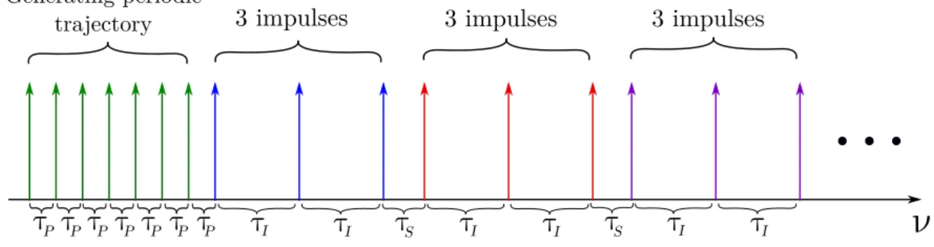
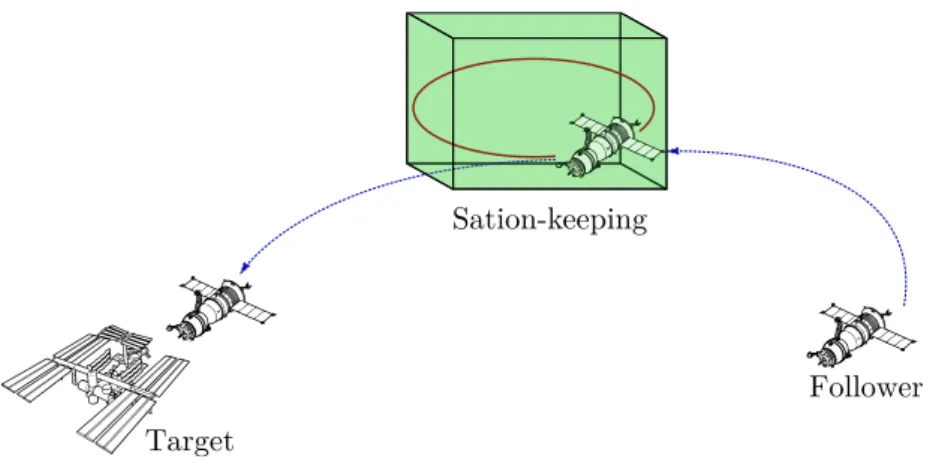
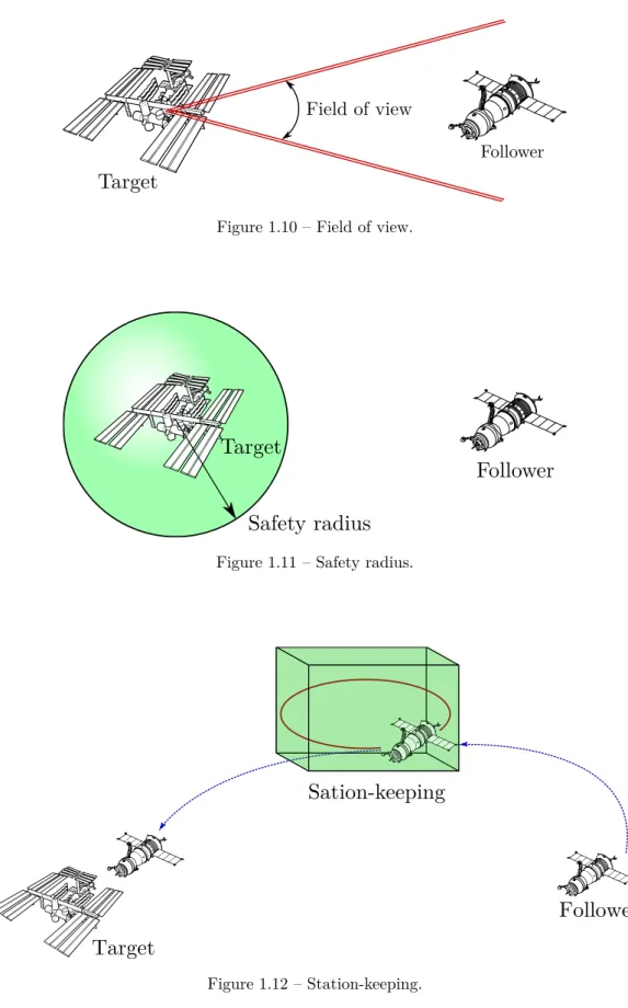
These approaching maneuvers are divided into several phases which are defined according to the inter-satellite distance, communication, visibility and other constraints. One of these phases is the so-called hovering phase [54,56–58, 71,72, 74,105] (see Fig. 4), in which the follower spacecraft is required to remain in a delimited region of the space relatively to the leader, while the mission control awaits for other events to be accomplished (measurements, synchronization, mission control decisions, visibility, etc).

Target

Follower Sation-keeping

Figure 4 – Hovering phases scheme.

One of the main objectives of this dissertation is the conception of autonomous guidance and control algorithms capable of complying with the complex restrictions of the rendezvous hovering phases, such as the time-continuous space constraints describing the hovering zone and the limitations of the thrusters. Moreover, the computation of the control actions must account for the minimization of fuel consumption, reducing the necessary fuel payload, ensuring feasibility and increasing the lifetime of the missions.

Another major concern of this work is to demonstrate that the proposed algorithms can be efficiently executed on devices dedicated to space applications. For this purpose, the control algorithms presented herein have to comply with the performances of a board containing a FPGA-synthesized LEON3 microprocessor. In fact, although this board is certified for space flights, it lacks computational power when compared to generic commercially available devices. The compilation chains and libraries used in the embedding of these algorithms are also provided.

A final and essential feature investigated in this work is mission safety. In order to ensure the successful mission accomplishment, the numerical results obtained during the execution of the proposed guidance and control algorithms must be validated4_{. The final developments of} this thesis focus on the application of validation techniques for obtaining validated bounds for the relative trajectories generated by the control actions computed by the proposed algorithms.

4

In the next section, the organization and main contributions of this work are presented.

Organization and contributions

In Chapter 1, the context and assumptions adopted for the hovering phases of the spacecraft orbital rendezvous missions are described and the mathematical formulation of the problem is established. The concepts of synthesis and simulation models are also introduced. The synthesis model is characterized by a structure which is adapted for the conception of con-trol algorithms and model predictive concon-trol strategies thanks to the existence of a formal propagation of the relative trajectories. On the other hand, the simulation model provides a high fidelity description of the physical phenomena involved in the orbital motion and, consequently, a more realistic representation of the spacecraft trajectories, being used to simulate the relative motion under the action of guidance algorithms. A first contribution of this work is the implementation of this simulation model in C and on Matlab R

/Simulink R

software, which led to the release of the two following simulators (freely available on-line): 1. A Matlab R/Simulink R non-linear simulator for orbital spacecraft rendezvous

applica-tions5 _[4];

2. A non-linear simulator written in C for orbital spacecraft rendezvous applications6 _[5]. In the end of Chapter 1, the synthesis model is used in the formulation of the fixed-time impulsive optimal guidance problem for relative motion in the context of the rendezvous hovering zone phases.

In Chapter2, the theoretical aspects of the resolution of the guidance problem formulated in Chapter1are discussed. With the goal of producing efficient optimization-based algorithms, three reformulations of the original problem are then proposed. The first reformulation is based on traditional discretization techniques, leading to a linear program (LP). The second one converts the original problem into a semi-definite program (SDP), using the relation between the cone of non-negative univariate polynomials and the cone of semi-definite positive matrices. The final proposition is an original contribution of this work, which consists in employing a geometrical approach based on the computation of the envelopes of the families of inequalities to describe the set of periodic constrained relative trajectories. This provides a reformulation of the original problem which relies on semi-algebraic functions, leading to a non-smooth optimization problem presented in the article:

5

https://hal.archives-ouvertes.fr/hal-01413328 6

3. Model predictive control for rendezvous hovering phases based on a novel description

of constrained trajectories [7], joint work with M. Joldeş, C. Louembet and F. Camps (research engineer, LAAS-CNRS), published in Proceedings of the 20th IFAC World

Congress (IFAC 2017).

Numerical methods for solving each of these optimization problems are given and their practical aspects are considered. These optimization methods are then coded in C and em-bedded on a board certified for space applications containing a FPGA-synthesized LEON3 microprocessor. The details about the employed libraries and compilation chains were pub-lished in the following article:

4. Embedding an SDP-based control algorithm for the orbital rendezvous hovering phases [24], joint work with F. Camps, M. Joldeş and C. Louembet, published in Proceedings of the 2018 25th Saint Petersburg International Conference on Integrated Navigation Systems (ICINS 2018).

In Chapter3a control strategy is proposed to steer the relative motion and keep it periodic and included in a given hovering zone. This strategy consists of a closed-loop model predictive control (MPC) algorithm, which is proven to make the relative movement converge to the hovering zone even when the presence of saturation constraints on controls may make the space window unreachable from the current state. The performance of this proposed control strategy is assessed via processor-in-the-loop simulations: the control computation is executed on a board containing an FPGA-synthesized LEON3 microprocessor and the propagation of the disturbed relative motion under uncertainties is performed on the previously mentioned simulators. These tests highlight the efficiency of the proposed control strategy in terms of control quality, numerical burden and rejection of disturbances. These original developments were presented in:

5. Stable Model Predictive Strategy for Rendezvous Hovering Phases Allowing for Control

Saturation [8], joint work with M. Joldeş, C. Louembet and F. Camps, submitted to the 2018 AIAA Journal of Guidance and Control and Dynamics and currently in revision (JGCD 2018).

Chapter4 is dedicated to the validation of numerical results obtained from the proposed on-board executed algorithms. In fact, during guidance and control procedures of orbiting spacecraft, the respect of positioning and space constraints is decisive for successful mis-sions achievement. Since result accuracy is essential for these procedures, the prevention

and estimation of errors arising from approximations and numerical computations become critical. In this context, a symbolic-numerical method for validating the solutions generated by the guidance and control algorithms is proposed. This approach provides error-bounded polynomial for the solutions of the linear ordinary differential equations (LODE) describing the linearized spacecraft relative motion. These developments led to the article:

6. Validated Semi-Analytical Transition Matrices for Linearized Relative Spacecraft

Dy-namics via Chebyshev Series Approximations [6], joint work with F. Bréhard (PhD student, LAAS-CNRS) and C. Gazzino (post-doctoral researcher, Technion Israel In-stitute of Technology), published in Proceedings of the 28th Space Flight Mechanics Meeting of the AIAA SciTech Forum (AIAA 2018).

Acknowledgments

This thesis was conducted in the Methods and Algorithms for Control group of the Laboratory for Analysis and Architecture of Systems (LAAS-CNRS), under the supervision of Mioara Joldeş and Christophe Louembet. The developments related to the embedding of algorithms on space dedicated hardware were only possible with the help and technical competences of Frédéric Camps, research engineer at LAAS-CNRS.

The FastRelax (ANR-14-CE25-0018-01) project of the French National Agency for Re-search (ANR) was the funding source of this work.

Modeling the problem

1.2.3 Deaconu’s parametrization and periodic relative trajectories . . . 23

1.3 Guidance of the relative motion. . . . 26

1.3.1 Space constraints: describing the hovering region . . . 27

1.3.2 Actuators and fuel consumption . . . 30

1.3.3 Optimal guidance problem formulation. . . 33

1.4 Conclusion . . . . 34

1.1

Introduction

In order to study the rendezvous mission context of a leader and a follower spacecraft orbiting a main body (the Earth, hereafter), mathematical models must be adopted to describe the relative motion, the actuators and the technological constraints for different purposes. Depending on the level of details and on the assumed hypothesis, several mathematical models can be employed in the description of these phenomena. First, the relative motion can be expressed by different state-space representations (e.g., Cartesian coordinates, orbital elements, equinoctial elements), using nonlinear or linearized dynamics. Then, since the object of study consists of mechanical systems, the significant forces acting over them must be inventoried. Concerning the gravitational forces, for example, the attraction between spacecraft themselves or between the spacecraft and other celestial bodies (Sun, Moon, Jupiter, etc.) can be taken into account or neglected. Other effects such as the Earth’s oblateness and non-homogeneous mass distribution, solar pressure or atmospheric drag may be taken into account as intrinsic dynamics or exogenous disturbances to the system. While the follower is usually equipped

with thrusters, the leader spacecraft can be considered active or passive depending on the ability of controlling its inertial orbit. Moreover, the thrusters can be modeled in several different ways, depending on the type of employed propulsion engines and their geometrical disposition. Depending on the rendezvous phase, many type of constraints can be accounted for: hovering zone, visibility cone, safety, orientation, control action dates, thrusters saturation and dead-zone, etc. This chapter aims to set the choices and specify the framework of this thesis.

In the sequel, the context and assumptions adopted for the hovering phases of the space-craft orbital rendezvous missions are described and the mathematical formulation of the problem is established. First, the concepts of simulation and synthesis models are introduced. The simulation model is more comprehensive with respect to the physical phenomena involved in the orbital motion and, consequently, provides a more realistic representation of the space-craft trajectories, being used to simulate the relative motion under the action of the conceived guidance algorithms; on the other hand, the synthesis model is less exhaustive and complex and is characterized, in this work, by linearized differential equations, which provides both a formal propagation and a structure adapted to the conception of control algorithms and model predictive control strategies.

The simulation model is obtained by the study of the two-body problem under Keplerian assumptions, which can be described by the Gauss planetary equations [47]. The orbital disturbances, that are not accounted in these models, are introduced as exogenous distur-bances and a simulator for the non-linear disturbed relative motion developed in C and on Matlab R/Simulink R is presented.

In order to obtain a synthesis model, the non-linear Tschauner-Hempel equations [100] are linearized [99,109] and an analysis of the impact of the linearization hypothesis on the evolution of the relative trajectories is carried out. Once a linear true anomaly-varying state-space representation of the relative motion is obtained, a parametrization of the relative trajectories is introduced [29]. This parametrization allows a straightforward characterization of the periodicity property, which is a very desirable feature from the point of view of fuel saving [44]. After that, the hovering region is described as a polytopic rectangular cuboid. The nature and geometrical placement of the propellers are discussed and the equations providing a characterization of the control actions and the fuel consumption are also exhibited. To conclude, the fixed-time impulsive optimal guidance problem for relative motion in the context of the rendezvous hovering zone phases is formulated.

1.2

Relative motion

The objective of this section is to detail the mathematical models that will be further employed in the description of the relative motion between spacecraft throughout this dissertation. In the next developments, the approach synthesis-simulation models is adopted.

The simulation model is used to separately simulate more realistically the behavior of each spacecraft involved in the rendezvous mission via the Gauss planetary equations (12 degrees of freedom, 6 orbital elements for each spacecraft). This model accounts for the intrinsic non-linearities and disturbances of the orbital motion. The relative motions is obtained by performing the passage from orbital elements to inertial states, then computing the difference between the positions and velocities of the leader and the follower spacecraft.

The synthesis model is obtained by performing a parametrization of the state vector employed in the simplified linearized Tschauner-Hempel equations for the relative motion (6 degrees of freedom, 3 relative position and 3 relative velocity coordinates). This variable change allows the conversion of the current relative state into parameters that are directly related to the shape of the relative orbits. This model is applied in the formulation of the fixed-time impulsive optimal guidance problem for the rendezvous hovering phases.

This choice is motivated by the fact that each of the models has advantages that can be exploited separately. The synthesis model is linear and admits a closed-form state-transition matrix that describes the propagation of the relative trajectories departing from a given initial state. This feature is interesting for model predictive control purposes, since it allows the computation of the evolution of the relative trajectory after the application of a control action. Moreover, the fact that this parametrization is related to the shape of the relative orbits leads to a formal description of the periodic relative orbits included in the hovering zone. The simulation model, even though more complex (since it does not admit a closed-from state transition and requires numerical integration), describes with more verisimilitude the motion and significant disturbances acting over each of the spacecraft separately. It provides, in a certain sense, a way of testing the behavior and robustnesses of the control strategies that are conceived and developed with less comprehensive models.

1.2.1 Simulation model

In this subsection, the simulation model is presented. It is obtained by first deducing the equations describing the movement of a single spacecraft orbiting a massive body in a Keple-rian framework. Then, the relevant orbital disturbances (the J2 effect and the atmospheric drag) are included in these equations as exogenous accelerations. The obtained equations are

then employed in the simulation of the dynamics of two spacecraft orbiting the same central body and the relative motion is then obtained by performing the difference between their trajectories. Finally, the obtained model for simulating the relative motion is implemented on C and on Matlab R

/Simulink R

.

1.2.1.1 Keplerian hypothesis

Consider two bodies in space with homogeneous mass distribution (m1, m2) and suppose that the first body is much more massive than the second m1 " m2 (e.g., the Earth and the International Space Station in Fig. 1.1) and that the only forces present in this system are the gravitational attractions (Keplerian motion).

Figure 1.1 – Two bodies in space.

In this case, the influence of the second body on the dynamics of the first one is considered negligible. Take an arbitrary inertial frame fixed on the first body FE “ pO, ~I, ~J , ~Kq and let

~

R be the position of the second body in this frame. By applying Newton’s second law of

movement, we obtain: m2 d2 dt2R~ptq “ ´ Gm1m2 } ~R_ptq}3 ~ R_{ptq ñ} d 2 dt2R~ptq “ ´ µ } ~R_ptq}3 ~ R_ptq, (1.1)

where G is the universal gravitational constant, µ “ Gm1 is the first body’s standard grav-itational parameter (e.g., for the Earth, µC “ p398 600.4405 ˘ 0.001q km3s´2 [92]). The general solutions of1.1are trajectories that assume the form of conic sections: circles, ellipses, parabolas and hyperbolas (more details in Fig. 1.2and [13, Chapters 3-4]).

Ellipse

Hyperbola

Parabola

Figure 1.2 – General solutions of the two body problem.

The following equation describes these general orbits in polar coordinates νptq and Rpνptqq:

R_{ptq “ } ~}R_{ptq} “} p 1 ` e cos νptq, e_{“ 0,} circular orbit 0 ă e ă 1, elliptical orbit e_{“ 1,} parabolic orbit e_{ą 1,} hyperbolic orbit (1.2)

where e is the eccentricity, ν is the true anomaly (position of the spacecraft on its orbit) and

p _{“ ap1 ´ e}2_{q the is the so-called semilatus rectum. For the elliptical and circular cases, a}

corresponds to the semi-major axis of the orbit.

In the sequel, we focus exclusively on the bounded periodic solutions: elliptical (and circular) orbits. In Fig. 1.3we depict a spacecraft moving in a generic elliptical orbit around Earth. Orbital plane Equatorial plane Line of nodes Vernal equinox direction North pole direction Perigee

Figure 1.3 – Orbital parameters.

that lies on the equatorial plane and has the direction of the vernal equinox (can be seen as the direction of the vector that goes from the center of the Earth to the center of the Sun when both are located on the equatorial plane), ~K is a vector perpendicular to the

equatorial plane, pointing towards the north pole and ~J is a vector that lies on the equatorial

plane that completes the orthogonal basis. The Earth centered orbital plane inertial frame FO“ pO, ~X, ~Y , ~Zq is such that ~X is equivalent to ÝÝÑOP, pointing towards the perigee of the

trajectory, ~Z is perpendicular to the orbital plane and ~Y completes the orthogonal basis

(omitted in Fig. 1.3).

The rotations allowing the passage from the frame FE to FOare depicted in Fig. 1.3and

given by: » — — — – ~ X ~ Y ~ Z fi ffi ffi ffi fl“ » — — — – 1 0 0 0 cos ω ´ sin ω 0 sin ω cos ω fi ffi ffi ffi fl loooooooooooomoooooooooooon rotation ofω around ~K » — — — – cos i ´ sin i 0 sin i cos i 0 0 0 1 fi ffi ffi ffi fl looooooooooomooooooooooon rotation ofi around ~J » — — — – 1 0 0 0 cos Ω ´ sin Ω 0 sin Ω cos Ω fi ffi ffi ffi fl loooooooooooomoooooooooooon rotation of Ω around ~K » — — — – ~ I ~ J ~ K fi ffi ffi ffi fl (1.3)

The parameters describing the configuration of the elliptical orbit with respect to the FE equatorial inertial frame and the position of the spacecraft on its orbit are the so-called classical orbital elements [77]:

OEc “

”

a, e, i, Ω, ω, νptq

ıT .

The size and shape of the orbit are given by the semi-major axis a and the eccentricity e. The line of nodes is given by the intersection between the orbital plane and the equatorial plane. The ascending node is the orbital position that lies on the line of nodes when the satellite enters the north half-space defined by the equatorial plane separation of the space. The orientation of the orbit with respect to the inertial frame is represented by the longitude

of the ascending node Ω (the angle between ~I and the ascending node), the argument of perigee ω (the angle between the ascending node. and the perigee direction) and the inclination i

(the angle between the orbital plane and the equatorial plane). Finally, the position of the satellite on its orbit is given by the true anomaly ν.

In absence of exogenous forces or disturbances, the free evolution of the position of a spacecraft on its elliptical orbit is expressed via the orbital elements by (1.2):

R_{ptq “ } ~}R_{ptq} “} ap1 ´ e

2_q 1 ` e cos νptq,

where the evolution of the true anomaly is given by the expression of its rate of change (see [37, Chapter 3.2] for further details):

dν dt “

c _µ

a3_{p1 ´ e}2_q3p1 ` e cos νq

2_{. (1.4)}

Evidently, this orbit can also be represented in the FOand FE frames by simply projecting

the vector ~R_{ptq on the vectors composing their respective bases.} 1.2.1.2 Non-Keplerian hypothesis

The previous obtained equations describe the shape of the spacecraft orbit as being a perfect ellipse (1.2). The speed at which a spacecraft travels on its orbit are given by the second and third Kepler’s laws (1.4). However, these equations do not account for all the effects acting over a spacecraft in orbit. Among these effect are:

• the atmospheric drag, which consists in the deceleration of the motion in the sense of the along track velocity provoked by the interaction of the spacecraft external area with the particles present in the atmosphere;

• the Earth’s gravitational disturbances provoked by its inhomogeneous mass distribution; • the gravitational pull of the Sun, the Moon and other planets;

• solar radiation pressure, which is the pressure applied on spacecraft’s surface provoked by the exchange of momentum between the object and the incoming radiation beam. These disturbances are included in the spacecraft orbital dynamics as accelerations pro-voked by exogenous disturbing forces. The evolution of the spacecraft’s orbital elements under these accelerations is given by the Gauss planetary equations [47]:

da dt “ 2 n?1 ´ e2 r´γzesin ν ` p1 ` e cos νqγxs de dt “ ? 1 ´ e2 n a „ ´γzsin ν ` ˆ

cos ν ` <sub>1 ` e cos ν</sub>e` cos ν ˙ γx  di dt “ ´ Rcos θ na2?<sub>1 ´ e</sub>2γy dΩ dt “ ´ Rsin θ na2?<sub>1 ´ e</sub>2<sub>sin i</sub>γy dω dt “ ? 1 ´ e2 n a e „ γzcos ν ` ˆ 1 `<sub>1 ` e cos ν</sub>1 sin ν ˙ γx  ` Rsin θ cos i n a2?<sub>1 ´ e</sub>2<sub>sin i</sub>γy dν dt “ n p1 ` e cos νq2 p1 ´ e2_q3{2 ` ? 1 ´ e2 n a e „ ´ cos ν γz´2 ` e cos ν 1 ` e cos ν γx  , (1.5)

where n “ c

µ

a3, θ “ ν ` ω and ~γ “ rγx, γy, γzs

T _{represents the sum of the accelerations}

provoked by disturbances in the Local-Vertical/Local-Horizontal frame LV LH “ pSl, ~x, ~y, ~zq,

depicted in Fig. 1.4. Evidently, if ~γ “ ~0, the same motion described by (1.2) and (1.4) is obtained: da dt “ de dt “ di dt “ dΩ dt “ dω dt “ 0, dν dt “ c _µ a3_{p1 ´ e}2_q3p1 ` e cos νq 2_.

Figure 1.4 – LVLH frame: the z-axis points from the spacecraft to the center of the Earth; the y-axis is normal to the orbital plane, negative in the direction of the angular momentum; the x-axis is mutually perpendicular to the y and z-axes.

The classical orbital elements employed in (1.5) may produce singularities (e “ 0 or i “ 0). In order to avoid it, a variable change is performed and the classical orbital elements are converted into the following modified equinoctial orbital elements:

OEeq “

”

p, f, g, h, k, L

ıT

, (1.6)

which can be obtained from the classical orbital elements via:

p _{“ ap1 ´ e}2_q f _{“ e cospΩ ` ωq,</sub> g <sub>“ e sinpΩ ` ωq,} h _{“ tanpi{2q cos Ω,} k _{“ tanpi{2q sin Ω,} L _{“ Ω ` ω ` ν.} (1.7)

The Gauss planetary equations (1.5) can then be rewritten using the equinoctial orbital elements, which produces the following equations [104]:

dOEeq

where: Aeq“ c_p µ » — — — — — — — — — — — — — — — — — — — — — — – 2p w 0 0 pw ` 1q cos L ` f w g_{ph sin L ´ k cos Lq} w ´ sin L pw ` 1q sin L ` g w ´ f_{ph sin L ´ k cos Lq} w cos L 0 ´s 2_{cos L} 2w 0 0 ´s 2_{sin L} 2w 0 0 ´hsin L ´ k cos L_w 0, fi ffi ffi ffi ffi ffi ffi ffi ffi ffi ffi ffi ffi ffi ffi ffi ffi ffi ffi ffi ffi ffi ffi fl (1.9) Beq “ „ 0, 0, 0, 0, 0, w2 p2 ?_µpT _{, (1.10)}

where w “ 1 ` f cos L ` g sin L.

In [34, Section 16.4], the author demonstrates that for flights at height of a few thousands of kilometers and less above the surface of the Earth, the perturbations related to the Moon and Sun pull are insignificant compared to the gravity anomalies and the second zonal harmonic of the geopotential (the so-called J2 effect). Also in [34, Section 17.3], it is shown that the solar radiation pressure is relevant only for small light-weight satellites orbiting at flight heights above 500 km. For all other satellites the perturbations produced by radiation pressure are small compared to the other disturbing effects. For the simulations performed throughout this dissertation, missions based on the International Space Station orbital parameters are employed [80] and, given that its flight height is below 500 km1_{, only the J}

2 effect and the atmospheric drag will be taken into account in the following developments:

• J2 disturbance: the acceleration provoked by the Earth’s flatness is given in the LVLH frame by [10,60]: ~γJ2 “ ´ 3µJ2R2e 2R4 » — — — — — — –

8ph sin L ´ k cos Lqph cos L ` k sin Lq p1 ` h2<sub>` k</sub>2<sub>q</sub>2 ´4ph sin L ´ k cos Lqp1 ´ h 2<sub>´ k</sub>2<sub>q</sub> p1 ` h2<sub>` k</sub>2<sub>q</sub>2 12ph sin L ´ k cos Lq2 p1 ` h2_{` k}2_q2 ´ 1 fi ffi ffi ffi ffi ffi ffi fl (1.11) 1 https://www.heavens-above.com/IssHeight.aspx

where J2 is the second degree term in Earth’s gravity potential and Re is the Earth’s

radius.

• Atmospheric drag: the disturbing acceleration provoked by the atmospheric drag is given in the LVLH frame by [10,60]:

~γd“ ´ ρ_pRqSCd 2m µ p a 1 ` 2pg sin L ` f cos Lq ` f2<sub>` g</sub>2 » — — — – 1 ` f cos L ` g sin L 0 ´f sin L ` g cos L fi ffi ffi ffi fl, (1.12)

where ρpRq is the atmospheric density and m, S and Cd are respectively the mass, the

cross sectional area and the drag coefficient of the spacecraft. The atmospheric density is given in function of the distance between the satellite and the center of the Earth by the following equation:

ρ_{pRq “ ¯}ρ exp ˆ Re´ R ` 400000 46830 ˙ , (1.13)

where ¯ρ is a constant that depends of the solar activity (2.2644 ˆ 10´12 for low and

3.5475 ˆ 10´11_{for high solar activity).}

1.2.1.3 Relative motion

In order to obtain the relative motion, the differential equations (1.8) are integrated for both leader and follower spacecraft independently, leading to a 12 degree of freedom model. At each integration step, the equinoctial orbital elements can be converted into the Cartesian inertial position and velocity via the following transformation:

xFE “ r s2pcos L ` α 2<sub>cos L ` 2hk sin Lq</sub> yFE “ r s2psin L ´ α 2<sub>sin L ` 2hk cos Lq</sub> zFE “ 2r s2ph sin L ´ k cos Lq 9 xFE “ ´ 1 s2 c<sub>µ</sub> ppsin L ` α 2_{sin L ´ 2hk cos L ` g ´ 2fhk ` α}2_gq 9 yFE “ ´ 1 s2 c_µ pp´ cos L ` α 2<sub>cos L ´ 2hk sin L ´ f ` 2ghk ` α</sub>2<sub>fq</sub> 9 zFE “ 2 s2 c<sub>µ</sub> pph cos L ` k sin L ` fh ` gkq, (1.14) where r “ p{w, s2_{“ 1 ` h</sub>2<sub>` k}2_{, and α}2_{“ h}2_{´ k}2_.

Then, the vector X “ rx, y, z, 9x, 9y, 9zsT _{representing the difference between the spacecraft’s}

positions and velocities projected on the leader’s LVLH frame is given by the following relations: » — — — — — — — — — — — — – x y z 9 x 9 y 9 z fi ffi ffi ffi ffi ffi ffi ffi ffi ffi ffi ffi ffi fl “ » — — — — — — — — — — — — – x~xl_{, ~p} FEy ´x~yl_{, ~p} FEy x~zl_{, ~p} FEy x~xl_{, ~v} FEy ` 9ν l_x~zl_{, ~p} FEy ´x~yl_{, ~v} FEy x~zl_{, ~v} FEy ´ 9ν l_x~xl_{, ~p} FEy fi ffi ffi ffi ffi ffi ffi ffi ffi ffi ffi ffi ffi fl (1.15)

where x¨, ¨y is the dot product in R3_,

~ pFE “ px f FE´ x l FE, y f FE ´ y l FE, z f FE ´ z l FEq

is the difference between the positions of the follower and leader spacecraft in the inertial frame, ~vFE “ p 9x f FE ´ 9x l FE, 9y f FE ´ 9y l FE, 9z f FE ´ 9z l FEq

is the difference between the velocities of the follower and leader spacecraft in the inertial frame, 9νl _{is the derivative with respect to time of the leader’s true anomaly and the unitary}

vectors ~xl_{, ~y}l_{, ~z}l _{compose the leader’s LVLH frame orthonormal basis and are given by the}

following expressions: ~ zl _{“ ´} px l FE, y l FE, z l FEq b pxl FEq 2_{` py</sub>l FEq 2<sub>` pz}l FEq 2, ~ xl _“ V~ }~V }, ~ yl _{“ ´} U~ }~U_}, where ~ T _“ p 9x l FE, 9y l I, 9zFlEq b p 9xl FEq 2_{` p 9y</sub>l FEq 2<sub>` p 9z}l FEq 2 ~ U _“ T~_{ˆ ~z}l ~ V _{“ ´~}U _{ˆ ~z}l (1.16) A simulator for the nonlinear disturbed movement based on the previously presented equations (1.8), (1.11), (1.14) and (1.15) was developed on Matlab R

/Simulink R

and in C. The Matlab R/Simulink R simulator is a modified version of the one proposed by Mounir

Kara-Zaitri in his PhD thesis [60, Chapter 4]. Some adjustments were performed in order to obtain a dedicated tool for simulating and developing control algorithms for the orbital spacecraft rendezvous in the case where the leader spacecraft is passive and the control applied on follower spacecraft is originally computed on the leader LVLH frame. On the other hand, the C version of the simulator is an original contribution of this work. For a given orbital rendezvous scenario, the output of both simulators is the evolution of the relative position and velocity between the two spacecraft, obtained by the integration of the Gauss equations for the orbital motion under the disturbances provoked by the Earth’s flatness (the J2 effect) and the atmospheric drag. These simulators are available at:

• C version: https://hal.archives-ouvertes.fr/hal-01410075 [5].

• Matlab R/Simulink R:

https://hal.archives-ouvertes.fr/hal-01413328 [4];

This simulator will be employed in the remainder of this dissertation for assessing the behavior of the proposed control algorithms in a non-linear and disturbed context.

1.2.2 Synthesis model

In this section, the model representing the relative dynamics between spacecraft that will be used throughout this dissertation for the development of control algorithms is presented. Several representations can be used for this purpose. For example, in the literature the differential orbital elements or modified versions of them are employed in formation flight applications [2,19]. Hereafter, the Cartesian local relative coordinates are chosen (6 degrees of freedom, 3 position and 3 velocity coordinates) for the initial study of the relative motion instead of the differential orbital elements. This choice is preferred for modeling problems in which space restriction are present [31, 50, 52], just as the rendezvous hovering phases problem. Nevertheless, later in this section, a parametrization of these Cartesian coordinates is introduced exhibiting an intrinsic relation between the obtained parameters and the shapes and boundedness of the relative orbits.

In the sequel, the equations describing the evolution of the relative motion between two spacecraft on elliptical orbits are presented (the reader may consult Appendix A for more details about the deduction of these equations). Let be Xptq “ rx, y, z, 9x, 9y, 9zsT _{the state}

vector containing the relative positions and velocities in the leader’s Local-Vertical/Local-Horizontal frame LV LH “ pSl, ~x, ~y, ~zq (see Fig. 1.5).

By applying Newton’s Second Law of motion to both spacecraft and subtracting the dy-namics of the leader from the follower spacecraft, the following system of nonlinear differential

Figure 1.5 – LVLH frame and rendezvous scheme. equations is obtained [100]: : x_{“ 2 9ν 9z ` :νz ` 9ν}2x_´b µx px2_{` y</sub>2<sub>` pR ´ zq}2_q3 : y_{“ ´}b µy px2_{` y</sub>2<sub>` pR ´ zq}2_q3 : z_{“ ´2 9ν 9x ´ :νx ` 9ν</sub>2z<sub>´</sub>b µpz ´ Rq px2<sub>` y}2_{` pR ´ zq}2_q3 ´ µ R2, (NLTH)

These are the so-called nonlinear Tschauner-Hempel equations. Assuming as linearization hypothesis that the distance between spacecraft is much smaller that the distance from the leader spacecraft to the center of the Earth:

a

x2_{` y</sub>2<sub>` z}2_{! R, (1.17)}

the linearized Tschauner-Hempel equations are obtained: : x_{“ 2 9ν 9z ` :νz ` 9ν}2_x´ µ R3x : y_{“ ´} µ R3y : z_{“ ´2 9ν 9x ´ :νx ` 9ν</sub>2<sub>z`} 2µ R3z. (LTH)

Let be ˜X_{pνq “ r˜x, ˜y, ˜z, ˜x}1, ˜y1, ˜z1_sT a new state vector such that:

˜

where the similarity transformation T pνq is given by: T_{pνq “} » – ρνI3 03 ´esνI3 pk2ρνq´1I3 fi fl . with k2 _“b µ

a3_p1´e2_q3, sν “ sinpνq and ρν “ p1 ` e cos νq.

By introducing these new variables in (LTH), the so-called simplified linearized Tschauner-Hempel equations [99,109] are obtained (for details, see AppendicesA.2 and A.3):

˜x2 _{“ 2˜z}1_, ˜y2_{“ ´y,} ˜z2 _“ 3 ρν˜z ´ 2˜x 1_, (SLTH) where p¨q1 _“ dp¨q dν , p¨q2“ d2 p¨q dν2 , dp¨q dt “ p¨q1ν,9 d2 p¨q dt2 “ p¨q2ν92` p¨q1ν.:

1.2.2.1 Evaluating the linearization hypothesis

In this section, the validity of the linearization hypothesis (1.17) is assessed. For that, let there be an initial true anomaly ν0 “ 0˝ and an initial relative state

X0pnq “ r10n, 10n, 10n, 0, 0, 0s. For a “ 7 ˆ 106, 8 ˆ 106 (

meters, e “ t0.04, 0.1u and

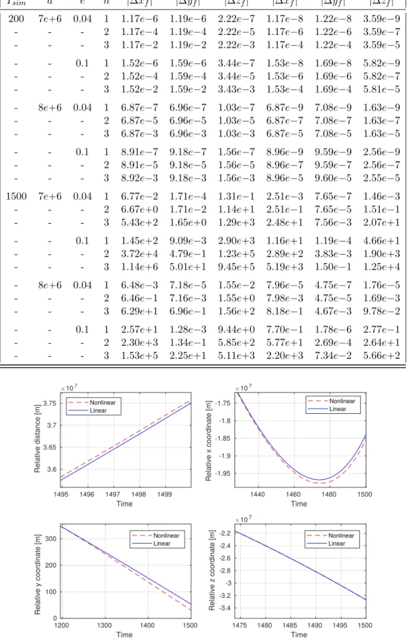
n_{“ t1, 2, 3u, the evolution of the relative trajectory is propagated during T}sim “ t200, 1500u seconds, considering the nonlinear (NLTH) and the linearized (LTH) relative dynamics2_{. The} absolute difference between the final states is presented in Table1.1 .

From Table1.1it is possible to remark that the absolute difference between the nonlinear and the linearized dynamics increases as the simulation time, the initial relative distance and the eccentricity increase; on the other hand, higher values of the semi-major axis result in higher distances between the leader spacecraft and the Earth, which makes the linearization hypothesis stronger and results in lower mismatches. For short simulation times (200 s), the committed errors are of the order of the centimeters for all configurations of initial states and eccentricities; however, for longer simulations (1500 s), the error can escalate to values equivalent to the Earth radius (see Fig. 1.6).

As a consequence of this, for certain scenarios, the relative trajectories obtained via linear propagation may present immense discrepancies with respect to those obtained via nonlinear propagation. In order to avoid these inconsistencies, control laws and theoretical studies synthesized using models based on the linearized Tschauner-Hempel equations should also be

2

The MATLAB R _{function ode45 is employed, with options RelTol}

“ 10´6

Table 1.1 – Evaluating the linearization hypothesis: difference between nonlinear and linearized Tschauner-Hempel equations.

Tsim a e n |∆xf| |∆yf| |∆zf| |∆ 9xf| |∆ 9yf| |∆ 9zf|

200 7e`6 0.04 1 1.17e´6 1.19e´6 2.22e´7 1.17e´8 1.22e´8 3.59e´9 - - - 2 1.17e´4 1.19e´4 2.22e´5 1.17e´6 1.22e´6 3.59e´7 - - - 3 1.17e´2 1.19e´2 2.22e´3 1.17e´4 1.22e´4 3.59e´5 - - 0.1 1 1.52e´6 1.59e´6 3.44e´7 1.53e´8 1.69e´8 5.82e´9 - - - 2 1.52e´4 1.59e´4 3.44e´5 1.53e´6 1.69e´6 5.82e´7 - - - 3 1.52e´2 1.59e´2 3.43e´3 1.53e´4 1.69e´4 5.81e´5 - 8e`6 0.04 1 6.87e´7 6.96e´7 1.03e´7 6.87e´9 7.08e´9 1.63e´9 - - - 2 6.87e´5 6.96e´5 1.03e´5 6.87e´7 7.08e´7 1.63e´7 - - - 3 6.87e´3 6.96e´3 1.03e´3 6.87e´5 7.08e´5 1.63e´5 - - 0.1 1 8.91e´7 9.18e´7 1.56e´7 8.96e´9 9.59e´9 2.56e´9 - - - 2 8.91e´5 9.18e´5 1.56e´5 8.96e´7 9.59e´7 2.56e´7 - - - 3 8.92e´3 9.18e´3 1.56e´3 8.96e´5 9.60e´5 2.55e´5 1500 7e`6 0.04 1 6.77e´2 1.71e´4 1.31e´1 2.51e´3 7.65e´7 1.46e´3 - - - 2 6.67e`0 1.71e´2 1.14e`1 2.51e´1 7.65e´5 1.51e´1 - - - 3 5.43e`2 1.65e`0 1.29e`3 2.48e`1 7.56e´3 2.07e`1 - - 0.1 1 1.45e`2 9.09e´3 2.90e`3 1.16e`1 1.19e´4 4.66e`1 - - - 2 3.72e`4 4.79e´1 1.23e`5 2.89e`2 3.83e´3 1.90e`3 - - - 3 1.14e`6 5.01e`1 9.45e`5 5.19e`3 1.50e´1 1.25e`4 - 8e`6 0.04 1 6.48e´3 7.18e´5 1.55e´2 7.96e´5 4.75e´7 1.76e´5 - - - 2 6.46e´1 7.16e´3 1.55e`0 7.98e´3 4.75e´5 1.69e´3 - - - 3 6.29e`1 6.96e´1 1.56e`2 8.18e´1 4.67e´3 9.78e´2 - - 0.1 1 2.57e`1 1.28e´3 9.44e`0 7.70e´1 1.78e´6 2.77e´1 - - - 2 2.30e`3 1.34e´1 5.85e`2 5.77e`1 2.69e´4 2.64e`1 - - - 3 1.53e`5 2.25e`1 5.11e`3 2.20e`3 7.34e´2 5.66e`2

1495 1496 1497 1498 1499 Time 3.6 3.65 3.7 3.75 Relative distance [m] 107 Nonlinear Linear 1440 1460 1480 1500 Time -1.95 -1.9 -1.85 -1.8 -1.75 R elativ e x coordi nat e [m] 107 Nonlinear Linear 1200 1300 1400 1500 Time 0 100 200 300 Nonlinear Linear 1475 1480 1485 1490 1495 1500 Time -3.4 -3.2 -3 -2.8 -2.6 -2.4 -2.2 107 Nonlinear Linear R elativ e y coordi nat e [m] R elativ e z coordi nat e [m]

tested on models based on the nonlinear dynamics. This conclusion corroborates the adopted strategy of using a synthesis model for conception of control algorithms and a simulation model for their "validation".

1.2.2.2 State-transition matrix

The linear true anomaly-varying system of equations (SLTH) can be expressed under the following state-space representation:

˜ X1_{pνq “} » — — — — — — — — — — — — – 0 0 0 1 0 0 0 0 0 0 1 0 0 0 0 0 0 1 0 0 0 0 0 2 0 ´1 0 0 0 0 0 0 3 ρν ´2 0 0 fi ffi ffi ffi ffi ffi ffi ffi ffi ffi ffi ffi ffi fl looooooooooooooooomooooooooooooooooon ˜ Apνq ˜ X_pνq (1.19)

Yamanaka and Ankersen propose in [109] a fundamental solution matrix (ϕpνq P R6ˆ6 non-singular, such that ϕpνq1_{“ ˜Apνqϕpνq) for this system:}

ϕ_{pνq “} » — — — — — — — — — — — — — – 1 0 _´cνp1 ` ρνq sνp1 ` ρνq 0 3ρ2νJν0pνq 0 cν 0 0 sν 0 0 0 sνρν cνρν 0 2 ´ 3esνρνJν0pνq 0 0 2sνρν 2cνρν´ e 0 3 ´ 6esνρνJν0pνq 0 ´sν 0 0 cν 0 0 0 cν` ec2ν ´sν´ es2ν 0 ´3e ˆ pcν` ec2νqJν0pνq ` sν ρν ˙ fi ffi ffi ffi ffi ffi ffi ffi ffi ffi ffi ffi ffi ffi fl , (1.20)

where sν “ sin ν and cν “ cos ν, Jν0pνq :“ żν ν0 dτ ρ_pτq2 “ c µ a3 t_{´ t}0 p1 ´ e2_q3{2, (1.21)

and ν0 is an arbitrary initial true anomaly of reference.

The propagation of an initial trajectory ˜X_pν0q can be performed via the state-transition matrix Φpν, ν0q “ ϕpνqϕ´1pν0q:

˜

where ϕ´1_pν 0q is given by: ϕ´1_pν0q “ » — — — — — — — — — — — — — — — – 1 0 _´3esν0p1 ` ρν0q ρν0pe 2 ´ 1q esν0p1 ` ρν0q e2 ´ 1 0 ecν0ρν0´ 2 e2 ´ 1 0 cν0 0 0 ´sν0 0 0 0 3sν0pρν0` e 2 q ρνpe2´ 1q ´ sν0p1 ` ρν0q e2 ´ 1 0 2e ´ cν0ρν0 e2 ´ 1 0 0 3pe ` cν0q e2 ´ 1 ´ 2cν0` ec 2 ν0` e e2 ´ 1 0 sν0ρν0 e2 ´ 1 0 sν0 0 0 cν0 0 0 0 <sub>´</sub>3ecν0` e 2 ` 2 e2 ´ 1 ρ2 ν0 e2 ´ 1 0 ´ esν0ρν0 e2 ´ 1 fi ffi ffi ffi ffi ffi ffi ffi ffi ffi ffi ffi ffi ffi ffi ffi fl . (1.23)

1.2.3 Deaconu’s parametrization and periodic relative trajectories

In this section, a transformation allowing the description of the relative state by a vector of parameters is introduced. This parametrization is demonstrated to be in a half-way between the representation of relative trajectories via Cartesian coordinates and via orbital elements, since it provides both a representation of the relative position and velocity between spacecraft and an interpretation of the shape and boundedness of these relative orbits.

In [28, Chapter 2], Deaconu remarked that the term ϕ´1_pν

0q ˜Xpν0q in (1.22) is a constant that only depends on the evaluation of ϕ and ˜X at ν0. Inspired by this observation, the author proposed the following variable change:

D_pνq“ » — — — — — — — — — — — — — — — – 0 0 _´3 ecν`e2`2 e2 ´ 1 ρ2 ν e2 ´ 1 0 ´ esνρν e2 ´ 1 0 0 3pe ` cνq e2 ´ 1 ´ 2cν`ec2ν`e e2 ´ 1 0 sνρν e2 ´ 1 0 0 3sνpρν`e2q ρνpe2´ 1q ´ sνp1`ρνq e2 ´ 1 0 2e ´ cνρν e2 ´ 1 1 0 <sub>´</sub>3 esνp1`ρνq ρνpe2´ 1q esνp1`ρνq e2 ´ 1 0 ecνρν´2 e2 ´ 1 0 cν 0 0 ´sν 0 0 sν 0 0 cν 0 fi ffi ffi ffi ffi ffi ffi ffi ffi ffi ffi ffi ffi ffi ffi ffi fl looooooooooooooooooooooooooooooooooooooooomooooooooooooooooooooooooooooooooooooooooon Cpνq ˜ X_pνq, (1.24)

where Dpν0q “ rd0pν0q, d1pν0q, d2pν0q, d3pν0q, d4pν0q, d5pν0qsT and Cpνq is equivalent to

ϕ´1_{pνq, but with some lines permuted: 1 Ñ 4, 2 Ñ 5, 4 Ñ 2, 5 Ñ 6 and 6 Ñ 1. Although this}

variable change may resemble like a mere replacement of the constant term ϕ´1_pν

0q ˜Xpν0q, the parameterization of the trajectories ˜X_{pνq by the vector Dpνq brings out many simplifications}

and advantages on the modeling of the problem:

by replacing ϕ´1_pν

0q ˜Xpν0q by Dpν0q in (1.22), the following equations are obtained: ˜xpνq “ p2 ` e cνqpd1pν0q sν´ d2pν0q cνq ` d3pν0q ` 3 p1 ` e cνq2d0pν0q Jν0pνq,

˜ypνq “ d4pν0q cν` d5pν0q sν,

˜zpνq “ p1 ` e cνqpd2pν0q sν` d1pν0q cν´ 3 e sνd0pν0q Jν0pνqq ` 2 d0pν0q.

(1.25)

and, as one can remark, the transition of the states ˜xpνq, ˜ypνq and ˜zpνq depends linearly on Dpν0q.

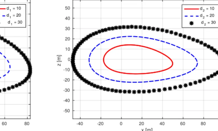
In Fig. 1.7 and Fig. 1.8, the shape of the relative trajectory associated to vector

D_{pνq “ r0, 10, 10, 10, 10, 10s}T for an eccentricity e “ 0.4 is illustrated by the

contin-uous red line. In each figure, the other two relative trajectories in blue dashed line and black stars are obtained by changing one parameter of D at time.

x [m] -40 -20 0 20 40 60 80 z [m] -50 -40 -30 -20 -10 0 10 20 30 40 50 d1= 10 d1= 20 d₁= 30

(a) Impact of d1 on the shape of the trajectory.

x [m] -40 -20 0 20 40 60 80 z [m] -50 -40 -30 -20 -10 0 10 20 30 40 50 d₂= 10 d₂= 20 d2= 30

(b) Impact of d2 on the shape of the trajectory.

x [m] -10 0 10 20 30 40 50 60 70 80 z [m] -30 -20 -10 0 10 20 30 d₃= 10 d₃= 20 d3= 30

(c) Impact of d3 on the shape of the trajectory.

Figure 1.7 – Impact of d1, d2 and d3 on the shape of the trajectory, d0“ 0 and e “ 0.4. From (1.24) and from Fig. 1.7and Fig. 1.8, one can observe that the first four entries of D (d0, d1, d2 and d3) characterize the shape of the trajectory in the XZ-plane and, the las two entries (d4 and d5), the shape of the Y-axis motion.

x [m] -30 -20 -10 0 10 20 30 40 50 60 y [m] -50 -40 -30 -20 -10 0 10 20 d4= 10 d₄= 20 d₄= 30

(a) Impact of d4on the shape of the trajectory.

x [m] -20 -10 0 10 20 30 40 50 60 y [m] -30 -20 -10 0 10 20 30 d₅= 10 d5= 20 d5= 30

(b) Impact of d5on the shape of the trajectory. Figure 1.8 – Impact of d4 and d5 on the shape of the trajectory, e “ 0.4.

2. A simple way to characterize the periodicity property: although the relative motion between spacecraft is not generally periodic, the periodicity property is inter-esting from the point of view of fuel consumption minimization [44]. This is mainly because in the absence of exogenous disturbances, once both spacecraft start to describe a periodic relative motion that respects the mission constraints, no further corrective control actions are required.

Hence, several control algorithms which minimize the fuel consumption require the generated relative trajectories to be periodic [7,9,22,44]. In order to develop control algorithms that minimize the fuel consumption, the generated relative trajectories are required to be periodic. However, in order to integrate this constraint in the formulation of the control algorithms, a mathematical description is needed.

One can observe that in (1.25), the only non-periodic divergent term in these equations is Jν0pνq, which always appears multiplied by the parameter d0pνq. Therefore, it is evident that a sufficient condition to obtain a periodic relative trajectory is to have

d0pνq “ 0, for all ν (see Fig. 1.9). However, from (1.26) we observe that, if for some

ν, d0pνq “ 0, then d0pνq “ 0, for all ν. We conclude then that a relative trajectory is periodic if and only if for some ν the computation of Dpνq “ Cpνq ˜X_{pνq produces a}

parameter d0 “ 0.

3. The state propagation of the vector Dpνq is simpler than the dynamics of ˜

X_{pνq: since for all ν, detpCpνqq ‰ 0, for a given ν, any vector ˜}X_{pνq has a single}

correspondent Dpνq and vice-versa. This means that in order to study the evolution of the state vector ˜X_{pνq, it suffices to analyze the behavior of Dpνq.}

x [m] -10 0 10 20 30 40 50 60 70 y [m] -30 -20 -10 0 10 20 30 d₀= 0 d₀= 1

(a) XY-plane view

x [m] -10 0 10 20 30 40 50 60 70 z [m] -30 -20 -10 0 10 20 30 d₀= 0 d₀= 1 (b) XZ-plane view Figure 1.9 – Link between d0and the periodicity property.

By manipulating (1.19) and (1.24) (see [28, Chapter 2] for details), we obtain the following dynamical system and state propagation representing the evolution of the vector of parameters: D1_{pνq “} » — — — — — — — — — — — — – 0 0 0 0 0 0 0 0 0 0 0 0 ´3e{ρ2 ν 0 0 0 0 0 3{ρ2 ν 0 0 0 0 0 0 0 0 0 0 0 0 0 0 0 0 0 fi ffi ffi ffi ffi ffi ffi ffi ffi ffi ffi ffi ffi fl looooooooooooooooomooooooooooooooooon ADpνq D_{pνq, or Dpνq “} » — — — — — — — — — — — — – 1 0 0 0 0 0 0 1 0 0 0 0 ´3eJν0pνq 0 1 0 0 0 3Jν0pνq 0 0 1 0 0 0 0 0 0 1 0 0 0 0 0 0 1 fi ffi ffi ffi ffi ffi ffi ffi ffi ffi ffi ffi ffi fl loooooooooooooooooooomoooooooooooooooooooon ΦD_pν,ν0q D_pν0q, (1.26)

and one can notice that the state propagation of Dpνq expressed in (1.26) is straight-forward compared to the one corresponding to the vector ˜X_{pνq, given by Φpν, ν}0q “

ϕ_pνqϕ´1_pν0q.

1.3

Guidance of the relative motion

The guidance problem for the rendezvous missions consists in computing the control actions and the generated relative trajectories that satisfy a set of constraints over the actuators and the trajectories, that are modeled by some system of nonlinear controlled dynamical equations:

d

or by some Linear Time-Varying (LTV) system of equations (as in (1.22), for example):

d

dtXptq “ AptqXptq ` Bptquptq, (1.28)

for which a linear state-transition is available for the modeling of the dynamics:

X_{ptq “ Φpt, t}0qXpt0q ` żt

t0Φpt, sqBpsqupsqds

(1.29) where Xptq P R6 _{is the relative state and uptq P R}3 _{is the vector that represents the control} actions (the free variable can be chosen as t or ν, since they are in a one-to-one correspondence). As discussed previously, the dynamics presented in (1.26) are used in the sequel to model the relative dynamics in the phase of conception of control algorithms and the disturbed nonlinear Gauss equations in equinoctial orbital elements (1.8), to simulate and validate the execution of the computed control actions.

So far, the nature of the terms Bptquptq and şt

t0Φpt, sqBpsqupsqds have not yet been

discussed. In this section, the physical model adopted to represent the spacecraft’s propellers, the effect of the application of the control actions on the relative dynamics and the metrics used to measure the fuel consumption is presented. Another subject treated in this section is the set of constraints that must be respected by the control actions and relative trajectories. The actuator constraints, as well as the space constraints of the rendezvous hovering phases, are also introduced. By the end of this section, all the necessary elements for the formulation of the guidance optimal problem for the rendezvous hovering phases will have been presented: a model for the propagation of the relative controlled dynamics, the fuel consumption that must be minimized, the space constraints describing the hovering zone and the restrictions on the control actions.

1.3.1 Space constraints: describing the hovering region

Several different types of space constraints must be satisfied by the relative motion between spacecraft during the rendezvous missions. Depending on the type of sensors used for the estimation of the relative distance and velocity of the spacecraft, a field of view is imposed to ensure the required conditions for the measurements (see Fig. 1.10). For close-range and proximity operations, a safety radius distance is imposed in order to avoid collisions (see Fig. 1.11). During the transition between checkpoints of the mission, the follower spacecraft must keep station in a delimited zone of the space relative to the leader spacecraft, the so-called hovering zone (see Fig. 1.12, more details in [37]). Hereafter, since the focus of