NEW DEVELOPMENTS IN COVARIANCE MODELING AND COREGIONALIZATION FOR THE STUDY AND SIMULATION OF NATURAL PHENOMENA
MIN LIANG
DÉPARTEMENT DES GÉNIES CIVIL, GÉOLOGIQUE ET MINES ÉCOLE POLYTECHNIQUE DE MONTRÉAL
THÈSE PRÉSENTÉE EN VUE DE L’OBTENTION DU DIPLÔME DE PHILOSOPHIÆ DOCTOR
(GÉNIE MINÉRAL) DÉCEMBRE 2015
c
ÉCOLE POLYTECHNIQUE DE MONTRÉAL
Cette thèse intitulée :
NEW DEVELOPMENTS IN COVARIANCE MODELING AND COREGIONALIZATION FOR THE STUDY AND SIMULATION OF NATURAL PHENOMENA
présentée par : LIANG Min
en vue de l’obtention du diplôme de : Philosophiæ Doctor a été dûment acceptée par le jury d’examen constitué de :
M. CHOUTEAU Michel, Ph. D., président
M. MARCOTTE Denis, Ph. D., membre et directeur de recherche M. GLOAGUEN Erwan, Ph. D., membre
DEDICATION
ACKNOWLEDGMENTS
Working as a Ph.D student of geostatistics was an amazing and challenging experience to me. During the five years, many people helped me in my research project. Without their support, this thesis would not be possible.
First I would like to express the deepest appreciation to my research director Professor Denis Marcotte, for his guidance, encouragement and financial support. Every time I met problem on my project, he always provides me his ideas and suggestions patiently. Without his contribution, I would not be able to complete my research work and this dissertation. I am deeply thankful to all members of the jury, professor Michel Chouteau, Xavier Emery and Erwan Gloaguen, for reading and evaluating this thesis.
I thank Nicolas Benoit from Gelogical Survey of Canada for providing data and technical supports.
I sincerely acknowledge China Scholarship Council, for offering me scholarship of studying. I also want to thank my colleagues and friends in the lab, Martine, Véronique, Pejman, Abderrezak, Eric, Alain, Clémence, Louis, Hassan and Raphael. Thank you for all information you shared, research suggestions, good restaurants, planting, baby caring and so on.
Moreover, I am especially grateful for my husband Xiaoyu for his support on my research project (discussion on geostatistics, suggestion and English improvement on my articles) and on my life (cooking delicious food). I also want to thank my parents for their constant encouragement and my daughter Sophie for her birth and smile which give me plenty of energy.
RÉSUMÉ
La géostatistique s’intéresse à la modélisation des phénomènes naturels par des champs aléa-toires univariables ou multivariables. La plupart des applications utilisent un modèle station-naire pour représenter le phénomène étudié. Il est maintenant reconnu que ce modèle n’est pas assez flexible pour représenter adéquatement un phénomène naturel montrant des comporte-ments qui varient considérablement dans l’espace (un exemple simple de cette hétérogénéité est le problème de l’estimation de l’épaisseur du mort-terrain en présence d’affleurements). Pour le cas univariable, quelques modèles non-stationnaires ont été développés récemment. Toutefois, ces modèles n’ont pas un support compact, ce qui limite leur domaine d’applica-tion. Il y a un réel besoin d’enrichir la classe des modèles non-stationnaires univariable, le premier objectif poursuivi par cette thèse.
Dans le cas multivariable, en plus du choix stationnaire, la plupart des applications sont limitées à l’utilisation du modèle linéaire de corégionalisation (LMC). Cette limitation est probablement due à 1) la facilité d’évaluer l’admissibilité du LMC, et 2) le manque de mé-thodes de simulation rapides pour les modèles qui ne sont pas LMC (N-LMC). Des progrès significatifs ont été faits sur le premier point récemment, mais moins sur le second. Par consé-quent, le second objectif principal de cette thèse est de fournir une méthode de simulation rapide pour N-LMC.
Cette thèse se compose principalement de trois articles. Le premier article utilise un modèle non-stationnaire univariable existant pour étudier le problème de l’estimation de l’épaisseur du mort-terrain en présence de nombreux affleurements. L’affleurement a une influence locale sur la distribution de l’épaisseur du mort-terrain car l’épaisseur y est nulle par définition. Le modèle non-stationnaire est ici utilisé pour limiter la distance d’influence des affleurements. À l’intérieur de cette distance d’influence, les paramètres de covariance sont supposés être des fonctions régulières simples de la distance à l’affleurement le plus proche. Au-delà de cette distance d’influence, la fonction de covariance de l’épaisseur de mort-terrain est supposée être stationnaire et l’influence des affleurements ne se fait plus sentir. La méthode est testée avec des données réelles. Les résultats montrent que le modèle non-stationnaire améliore la précision et le réalisme de l’estimation, en particulier à proximité des affleurements.
Le deuxième article introduit de nouvelles fonctions non-stationnaires avec support compact, remplissant ainsi le premier but principal de la thèse. Les fonctions développées sont issues du modèle sphérique. Elles sont dérivées par convolution d’hypersphères dont le rayon varie spatialement en <n. On applique ensuite une transformation de Radon dont l’ordre contrôle
la continuité de la fonction de covariance résultante. Les expressions explicites des cova-riances non-stationnaires isotropes sont dérivées pour les modèles sphériques, cubiques, et penta-sphériques. Aussi une méthode de simulation des modèles non stationnaires utilisant la moyenne pondérée d’un bruit blanc gaussien est décrite pour les cas isotrope et anisotrope. Le troisième article présente une méthode de simulation efficace pour N-LMC basée sur la transformée de Fourier rapide (FFT) et la moyenne mobile (GFFTMA), réalisant ainsi le deuxième but principal de la thèse. Cette méthode permet de simuler des variables avec des structures spatiales différentes. Dans le domaine spectral, les matrices de densités sont décomposées séparément, en valeurs propres-vecteurs propres, à chaque fréquence discrète. Le champ corrélé est obtenu par la multiplication, à chaque fréquence, de la racine carrée de la matrice spectrale par les spectres de bruits blancs gaussiens suivi d’une transformée inverse de Fourier. Ceci permet d’imposer les structures spatiales directes et croisées désirées pour chaque variable. Cette méthode possède une complexité Nlog (N) (N, le nombre de pixels à simuler). La méthode GFFTMA est testée sur des exemples synthétiques à deux ou trois variables et formés de différentes combinaisons de modèles parmi les sept modèles de base disponibles. Tout les cas testés montrent des réalisations dont les variogrammes expérimentaux directs et croisés reproduisent très bien le modèle cible.
Les trois articles utilisent comme étude de cas le problème de l’estimation et la simulation de l’épaisseur du mort-terrain dans les basses terres de Saint-Laurent et de la l’est de la Montérégie, Québec, Canada. Les nouveaux outils développés dans cette thèse permettent de mieux étudier les phénomènes naturels aussi bien pour le cas univariable, où les modèles non stationnaires à support compact offrent plus de flexibilité, que dans le cas multivariable stationnaire, où une méthode de simulation non-LMC efficace basée sur la FFT a été déve-loppée. Ensemble, ces outils devraient permettre d’améliorer la modélisation des phénomènes naturels.
ABSTRACT
Geostatistics focus on modeling natural phenomena by univariate or multivariate spatial random fields. Most applications rely on the choice of a stationary model to represent the studied phenomenon. It is now acknowledged that this model is not flexible enough to adequately represent a natural phenomenon showing behaviors that vary substantially in space (a simple example of such heterogeneity is the problem of estimating overburden thickness in the presence of outcrops). For the univariate case, a few non-stationary models were developed recently. However, these models do not have compact support, which limits in practice their range of application. There is a definite need to enlarge the class of univariate non-stationary models, a first goal pursued by this thesis.
In the multivariate case, in addition to the stationary choice, most applications are limited to use of the linear model of coregionalization (LMC). This limitation is probably governed by 1) the ease of assessing the admissibility of the LMC, and 2) the lack of availability of fast simulation methods for models that are not LMC (N-LMC). Significant progress were made on the first point recently, but not much on the second. Hence, the second main goal of this thesis is to provide a fast simulation method for stationary non-LMC.
This thesis is mainly composed of three articles. The first article uses the existing univariate non-stationary model to study the problem of estimating the overburden thickness in presence of many outcrops. The outcrop has local influence on overburden thickness distribution as the thickness value is zero on the outcrop. The non-stationary model is used to restrict the distance of influence of outcrops. Within this distance of influence, covariance parameters are assumed to be simple functions of the distance to the nearest outcrop. Beyond the distance of influence of outcrops, the thickness covariance is assumed stationary. The method is tested with real data. The results show that the non-stationary model improves the precision of estimation and provides realistic map, especially at points close to outcrops.
The second article develops new non-stationary functions with compact support, thus fulfill-ing the first main goal of the thesis. The developed functions include the non-stationary form of the spherical family model. It is derived by convolving hyperspheres (with spatially vary-ing radius) in <nfollowed by a Radon transform. The order of the Radon transform controls the differentiability of the covariance functions. Closed-form expressions for the isotropic non-stationary covariances are derived for the spherical, cubic, and penta-spherical models. Also a simulation method of the non-stationary models is described by weighted average of independent standard Gaussian variates in both the isotropic and the anisotropic case.
The third article presents a very fast simulation method for N-LMC, the general fast Fourier transform and moving average (GFFTMA), thus realizing the second main goal of the the-sis. This method makes available to simulate variables following different spatial structures. In spectral domain, the spectral density matrices are eigen-decomposed separately at each discrete frequency. Correlated spectrum for each variable is produced by the decomposed ma-trices multiplied with the spectrum of Gaussian white noise. Then taking the inverse Fourier transform, the random field of each variable in spatial domain is created. The CPU- time of this method increases as N log(N ) (N , the number of pixels to simulate). The GFFTMA is tested in simulation of synthetic examples with two and three variables for different combi-nations of the seven available models. All the realizations produced fit the desired covariance model well.
The three articles use as illustrative case study the problem of estimating and simulating the overburden thickness in the Saint-Laurence lowlands, Montérégie Est, Québec, Canada. As a whole, this thesis provides new tools to better study the natural phenomena both in the univariate case, where compactly supported non-stationary models offer more flexibility, and in the stationary multivariate case, where an efficient FFT based non-LMC simulation method is derived. Together, they should help improve modeling of natural phenomena.
TABLE OF CONTENTS DEDICATION . . . iii ACKNOWLEDGMENTS . . . iv RÉSUMÉ . . . v ABSTRACT . . . vii TABLE OF CONTENTS . . . ix
LIST OF TABLES . . . xiii
LIST OF FIGURES . . . xiv
LIST OF ABBREVIATIONS AND SYMBOLS . . . xv
CHAPTER 1 INTRODUCTION . . . 1
1.1 Basic concepts . . . 1
1.2 Research problems . . . 2
1.3 Objectives and contributions of the thesis . . . 2
1.4 Structure of the thesis . . . 3
CHAPTER 2 LITERATURE REVIEW . . . 5
2.1 Non-stationary model . . . 5
2.1.1 Stationary model . . . 5
2.1.2 Non-stationary covariance functions . . . 6
2.2 Stationary compactly supported covariance functions . . . 9
2.2.1 Direct construction of compactly supported radial functions . . . 10
2.2.2 Development of compactly supported covariance functions in geostatistics 10 2.3 Multivariate modeling and simulation . . . 11
2.3.1 The linear model of coregionalization . . . 12
2.3.2 The non-linear model of coregionalization and its simulation . . . 13
CHAPTER 3 THESIS ORGANIZATION . . . 16
3.1 The first article . . . 16
3.3 The third article . . . 17
3.4 Consistency among the papers . . . 18
CHAPTER 4 THEORETICAL BACKGROUND . . . 20
4.1 Estimation and simulation techniques . . . 20
4.1.1 Kriging . . . 20
4.1.2 CoKriging . . . 22
4.1.3 Simulations . . . 23
4.2 The Non-stationary covariance functions based on kernel convolution . . . . 29
4.3 Compactly supported functions . . . 30
4.3.1 Spherical family model and Euclid’s hat . . . 31
4.3.2 Wu’s function . . . 32
4.3.3 Wendland’s function . . . 33
CHAPTER 5 ARTICLE 1 : A COMPARISON OF APPROACHES TO INCLUDE OUTCROP INFORMATION IN OVERBURDEN THICKNESS ESTIMATION . 35 5.1 Abstract . . . 35
5.2 Introduction . . . 36
5.3 Methodology . . . 38
5.3.1 Non-Stationary Covariance Model . . . 38
5.3.2 Thickness Estimation . . . 40
5.3.3 Performances Evaluation . . . 42
5.4 Case Study . . . 43
5.4.1 Study area . . . 43
5.4.2 Model Parameters and results . . . 43
5.5 Discussion . . . 46
5.6 Conclusion . . . 49
5.7 Acknowledgements . . . 49
5.8 Appendix A . . . 49
References . . . 53
CHAPTER 6 ARTICLE 2 : A CLASS OF NON-STATIONARY COVARIANCE FUNC-TIONS WITH COMPACT SUPPORT . . . 56
6.1 Abstract . . . 56
6.2 Introduction . . . 56
6.3.1 The spherical family . . . 60
6.3.2 Covariance functions obtained by Radon transform . . . 61
6.4 Non-stationary compactly supported covariance functions . . . 62
6.4.1 Non-stationary isotropic covariance model by convolution . . . 62
6.4.2 Closed-form expression in the non-stationary isotropic case for the spherical model . . . 63
6.4.3 Other non-stationary isotropic models of the spherical family model . 66 6.4.4 Computation of non-stationary anisotropic spherical family covariance models . . . 66
6.5 Examples . . . 67
6.5.1 Correlation . . . 67
6.5.2 Unconditional simulation . . . 67
6.5.3 Conditioning the realizations . . . 73
6.5.4 Sparse covariance matrix . . . 73
6.6 Case study . . . 75
6.7 Conclusion and discussion . . . 78
6.8 Acknowledgment . . . 82
6.9 Appendix - Closed-form expressions for the cubic and the penta-spherical models 83 References . . . 85
CHAPTER 7 ARTICLE 3 : SIMULATION OF NON-LINEAR COREGIONALIZA-TION MODELS BY FFTMA . . . 88
7.1 Abstract . . . 88
7.2 Introduction . . . 89
7.3 Methodology . . . 90
7.3.1 The FFTMA in the multivariate case . . . 91
7.3.2 Post-conditioning by cokriging . . . 93
7.3.3 Models with asymptotic range . . . 94
7.3.4 Test of GFFTMA . . . 94
7.3.5 Computing time . . . 95
7.3.6 Memory usage . . . 100
7.4 Case Study - Overburden thickness simulation . . . 101
7.4.1 Comparison of statistics of conditional realizations by N-LMC model and univariate simulation . . . 103
7.5 Discussion . . . 106
7.7 Acknowledgments . . . 108
7.8 Appendix - usage of GFFTMA . . . 108
References . . . 110
CHAPTER 8 GENERAL DISCUSSION . . . 113
CHAPTER 9 CONCLUSION AND FUTURE WORK . . . 116
9.1 Conclusion . . . 116
9.2 Limitations and future work . . . 116
LIST OF TABLES
Table 5.1 Statistics of estimates by stationary (K-S and K-SO) and non-stationary
kriging (K-NS) . . . 46
Table 5.2 Non-Stationary covariance model parameters for each point . . . 49
Table 5.3 Non-Stationary covariances for K-NS and kriging weights . . . 50
Table 5.4 Stationary covariances for K-SO and kriging weights . . . 51
Table 6.1 Normalizing constants in Eq. 6.14 . . . 62
Table 6.2 Computation time (seconds) of isotropic simulations by spherical model 73 Table 6.3 Sparsity and memory consumption for a simulated field of size 100 × 100 . . . 74
Table 6.4 Statistics of estimates by stationary and non-stationary kriging . . . 78
Table 7.1 Models used in Figs 7.2-7.5 and Fig. 7.9 . . . 100
Table 7.2 Maximum size of simulated field as a function of available RAM above overhead memory required by operating system and Matlab (for nsim = 1, na = 100, p = 2) . . . 101
LIST OF FIGURES
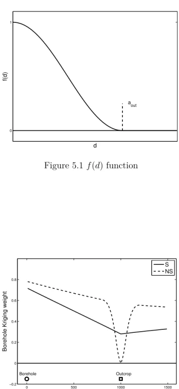
Figure 5.1 f (d) function . . . . 41 Figure 5.2 Borehole kriging weights for stationary and nonstationary kriging with
aout = 200 m and exponential stationary covariance with C0 = 1, C = 2
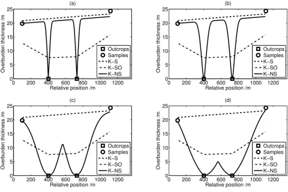
and a = 2000 m. . . . 41 Figure 5.3 Thickness profiles by stationary and nonstationary kriging with aout of
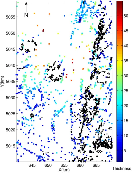
(a) 60 m, (b) 120 m, (c) 500 m and (d) 1000 m. . . 42 Figure 5.4 Map of study area and sample data. Borehole data as squares and
outcrops as black dots . . . 44 Figure 5.5 Training set cross-validation MAE for the non-stationary covariance
model as a function of aout. . . 45
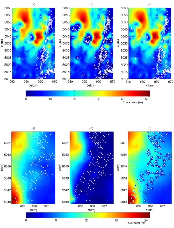
Figure 5.6 Estimation maps by (a) K-S, (b) K-SO and (c) K-NS. White dots represent outcrops. Top row, the entire study area. Bottom row, zoom in the outlined rectangle. . . 47 Figure 5.7 Correlations between K-S, K-SO and K-NS as a function of the distance
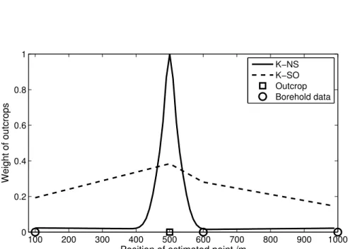
to the nearest outcrop. Only the points within that distance are kept when computing the correlations. . . 48 Figure 5.8 Kriging weight assigned to outcrop as a function of the estimation point
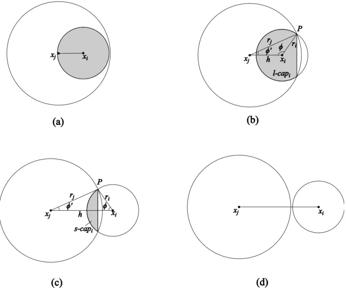
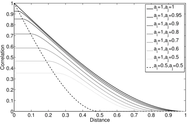
for K-SO and K-NS . . . 51 Figure 6.1 General view of circle-circle intersection . . . 64 Figure 6.2 Spherical NS correlation between points xi(with range ai) and point xj
(with range aj) as a function of distance between the points (||xi−xj||).
For ||xi− xj|| < (ai− aj)/2 (with ai ≥ aj), the correlation is constant
at qa3
j/a3i. . . 68
Figure 6.3 NS correlation ((solid lines) and stationary correlation (dashed lines) between points xi (where range ai = 1) and point xj (where range aj =
1 − 0.5|hij|) as a function of distance between the points (hij = ||xi−
xj||) for the spherical, the cubic and the penta-spherical models. For
comparison, the stationary correlation functions with an intermediate range of 0.75 are also illustrated. . . 69 Figure 6.4 Non-stationary isotropic realizations by (a) spherical model, (b) cubic
model and (c) penta-spherical model. In all simulations, range of model is changing from 30 on top to 5 on bottom. . . 70
Figure 6.5 Comparison of simulated variogram and the theoretical. For each reali-zation, the variogram is computed along the vertical between the pixels on row y = 200 (where a = 30) and the pixels on row y = 200−distance (where a = 30 − distance200 × (30 − 5)). . . 71 Figure 6.6 Non-stationary anisotropic realizations by (a) spherical model, (b)
cu-bic model and (c) penta-spherical model. In all simulations, the azimuth and range of a point are functions of location. The direction of the main continuity follows the azimuth and the range increases linearly from 5 pixels at the center to 50 pixels at the circumference. The range in the tangential direction is set to 1/3 the range in the radial direction. (d) shows the local structure by illustrating the local support of the weight function. . . 72 Figure 6.7 Three 1D conditional realizations for cubic model with range 10 for
x < 50 and range 2 for x > 50. . . . 74 Figure 6.8 Map of study area and sample data. Size of symbols is proportional
to thickness value. Black and gray symbols represent sample data in different geological domain. . . 76 Figure 6.9 Map of correlation range evolution. . . 76 Figure 6.10 Covariance contours on 10 points in the study area. The black dashed
line represents the boundary of the two geological domains. . . 77 Figure 6.11 Estimation maps at the whole area by (a) stationary kriging with global
model, (b) stationary kriging with local model in each domain and (c) non-stationary kriging with a total 3 km wide transition area (between dashed lines), centered at the contact between the geological domains, where the model parameters change continuously. The white points represent data locations. The black line indicates the contact of two geological domains. . . 79 Figure 6.12 Zoomed maps (area outlined in Fig. 6.11) by (a) stationary kriging with
global model, (b) stationary kriging with local model in each domain and (c) non-stationary kriging with a transition area in which the model parameters change continuously. . . 80 Figure 6.13 Kriging standard deviation by (a) stationary kriging with global model,
(b) stationary kriging with local model in each domain and (c) non-stationary kriging with a transition area in which the model parameters change continuously. . . 81
Figure 6.14 NS isotropic covariance for the cubic and the penta-spherical model for various supports. . . 84 Figure 7.1 Example of slope discontinuity at practical range ap after periodization
of the exponential model. . . 95 Figure 7.2 One realizations of v1 and v2 (top row) and the direct and-cross
va-riograms. Case 1 of Table 7.1 mixing exponential, Generalized Cauchy with ν = 2 and K-Bessel with ν = 1. Mean variogram is computed by combining E-W and N-S directions over 200 realizations. Only the first 25 individual realization variograms (light gray) are shown. . . 96 Figure 7.3 One realization of v1 and v2 (top row) and the direct and
cross-variograms. Case 2 of Table 7.1. Mean variogram is computed by com-bining E-W and N-S directions over 200 realizations. Only the first 25 individual realization variograms (light gray) are shown. . . 97 Figure 7.4 One realization of v1, v2 and v3 (top row) and the direct and
cross-variograms. Case 3 of Table 7.1. Mean variogram is computed by com-bining E-W and N-S directions over 200 realizations. Only the first 25 individual realization variograms (light gray) are shown. . . 98 Figure 7.5 One realization of v1 and v2 (top row) and the direct and
cross-variograms. Case 4 (with geometric anisotropy) in Table 7.1. Horizontal direction (left column) and vertical direction (right column). Mean va-riogram is computed over 200 realizations. Light gray : vava-riograms for the first 25 realizations . . . 99 Figure 7.6 Evolution of computing time as a function of a) the number of
simu-lated pixels and b) the number of realizations (for a field of 200 x 200 pixels). Simulation of two variables for four different models in a) and a spherical model with range 100 in b). . . 101 Figure 7.7 Map of sample data. Gray dots : boreholes in geological domain A,
black dots : boreholes in geological domain B. The area covered by simulation in Fig. 7.10 is outlined (dashed line) . . . 102 Figure 7.8 Model fitting for direct and cross variograms of log(thickness) and one
latent field representing the geological domain information. . . 104 Figure 7.9 Comparison of the direct and cross variograms of log(thickness) and
the latent variable between 30 realizations and the theoretical model. 105 Figure 7.10 Realizations of univariate simulation (left) and N-LMC simulation (right).
LIST OF ABBREVIATIONS AND SYMBOLS
FFTMA Fast Fourier transform moving average
GFFTMA General fast Fourier transform moving average LMC Linear model of coregionalization
N-LMC Non-linear model of coregionalization
ME Mean error
MAE Mean absolute error RMSE Root mean square error
K-S Kriging based on stationary model without outcrop information K-SO Kriging based on stationary model incorporating outcrop information K-NS Kriging based on non-stationary model incorporating outcrop
informa-tion
a Correlation range
d Distance
f Function
g Covariogram
hij Distance vector between xi and xj
k Kernel function
k Covariance vector between observations and aim point
m Mean n Number p Proportion x Coordinate of a point A Amplitude C Covariance function
CS Stationary covariance function
CN S Non-stationary covariance function
Cov Covariance
D(f ) Differential operator
E Expectation
F Facies
F Fourier transform
I Incomplete beta function I Indicator function
I(f ) Integral operator
K Covariance matrix among observations Kν Bessel function of order ν
L Lagrange function P Transition kernel Prob Probability
R Correlation
RS Stationary correlation function RN S Non-stationary correlation function
Rf Radon transform
S Power spectral density function
V Volume
Var Variance
X Euclid’s hat
Xi Poission point process
Y (x) Random function Z(x) Random function Z∗(x) Estimate of Z(x) ZCS Conditional simulation
ZS Unconditional Simulation
ZS∗ Estimate using simulation
α Weight of secondary variable in cokriging δ Gaussian random variable
λ Weight in Kriging γ Variogram µ Drift µl Lagrange multiplier ρ Correlation function σ Standard deviation ω Dilution function ϕW u Wu’s function ϕW e Wendland’s function Σ Kernel Matrix
<n Real space in n-dimensions
CHAPTER 1 INTRODUCTION
1.1 Basic concepts
Many natural phenomena can be characterized by spatial variables, such as soil properties, the concentration of pollutants, or the temperature in a region. The studies of spatial va-riables often involve to determine the value on every point based on imperfect understanding of the phenomena and limited known information. This brings uncertainty into the study. Geostatistical methods can describe the spatial structure hidden by the randomness of spatial variables, such as orientation, smoothness of transition, and so on. To characterize the spatial structure in a simple way, some hypotheses are commonly assumed including typically : 1) the stationarity of the covariance model for univariate study, and 2) the linear model of core-gionalization for multiple variables. These assumptions limit the applicability of the methods in a complex real world.
Stationarity is a common assumption in geostatistics. It means that the spatial structure of a variable, typically the mean and the covariance, do not change with locations over the study domain. In fact, many phenomena exhibit local varying structures. For example, variation of the annual precipitation is much greater in mountain than in flat plain (Paciorek and Scher-vish, 2006). Likewise, the distribution of atmospheric pollutants show large spatial variability depending on the source location, meteorology and the chemical reactions between the source and receptor (Fuentes, 2001). Another typical example is distribution of overburden thick-ness over a domain. In a plain area, the overburden usually has a uniform thickthick-ness. But the presence of outcrops interrupts the continuity, which leads to a locally different distribution of overburden thickness in the vicinity of the outcrops. To better quantify these location dependent structures, non-stationary models emerged and became an appealing solution in recent decades. Despite the powerfulness, computational limitations can happen when data is abundant as the existing non-stationary model do not have compact support. The resulting covariance matrix then becomes large and non-sparse. One has to resort the local neighbo-rhoods to alleviate the problem however that may generate undesirable discontinuities. There is a definite need for non-stationary compactly supported covariance models as an alternative to local neighborhood approaches.
In many instances, more than one variable are studied simultaneously. For example, the geophysical data can reflect the intrinsic properties of overburden and could be considered to better estimate the overburden thickness (Hunter et al., 1984; Caron et al., 2013; Blouin et al., 2013). The linear model of coregionalization (LMC) is commonly used in modeling of
correlated multiple variables. It requires each covariance of variables is a linear combination of the same spatial model. The LMC is practical in limited cases, such as geochemistry and study of animal abundance (Chilès and Delfiner, 1999). In fact, the non-linear model of coregionalization (N-LMC) describes more general and common situations, where variables can follow entirely different structures. For example, in geophysics, the density and magnetic susceptibility are closely correlated while their indicators, gravity and magnetic field data, follow different spatial structures. The gravity field has smoother behavior than the magnetic susceptibility (Maus, 1999). As another example, in geology the spatial field of overburden thickness usually can be described by a model which has linear behavior at the origin. One of its correlated variable, geological domain can be modeled by thresholding a continuous Gaussian variable. To obtain realistic geological domains, it is needed to adopt a variogram with parabolic behavior for the latent variable, hence necessitating a N-LMC to simulate jointly the thickness and the latent variable. To be practical, an efficient method is needed to simulate such fields with N-LMC.
1.2 Research problems
The study of natural phenomena is often limited in the univariate case to methods using stationary models. In the multivariate case, the stationary LMC is by far the most often used model. These models lack flexibility and are not deemed sufficient to represent adequately the complexity of many natural phenomena. There is a definite need to enlarge the class of univariate non-stationary models and to escape from the LMC straitjacket to adequately represent the studied natural phenomena.
More specifically, the following research problems arise :
1. In univariate case, how to model the heterogeneity of a random field with a non-stationary covariance ? How to define non-non-stationary models with compact support that allows to obtain sparse covariance matrices ? How to simulate efficiently these non-stationary fields ?
2. In multivariate case, how to simulate N-LMC field efficiently ?
1.3 Objectives and contributions of the thesis
The objectives of this thesis are :
1. To develop a non-stationary model to incorporate the outcrop information in overbur-den thickness estimations.
2. To develop a class of compactly supported non-stationary covariance functions. 3. To develop an approach of simulation based on the non-stationary covariance model. 4. To develop an efficient method of multivariate simulation of N-LMC.
This thesis achieves the following original contributions :
1. A non-stationary model which includes outcrops position in overburden thickness es-timation. It produces realistic maps and improves the thickness estimation precision. 2. A class of non-stationary covariance functions with compact support, of which a special case is a non-stationary form of spherical family model. The non-stationary model is applied in overburden thickness estimation incorporating classification of the geological domain and enables a reduction of the estimation error and a more realistic transition between two geological domains.
3. A method for simulating non-stationary models with compact support in both isotro-pic and anisotroisotro-pic cases.
4. A general method to simulate multivariate fields with N-LMC based on the fast Fourier transform - moving average method (FFTMA).
1.4 Structure of the thesis
This thesis consists of nine chapters. The first chapter provides a brief overview of the thesis, including basic introduction, research problems, objectives, contributions and structure. Chapter 2 presents a literature review encompassing the origin and development of major topics of the thesis.
Chapter 3 describes the organization of the thesis and the pertinence of the articles with regards to the objectives of the thesis.
Chapter 4 introduces theoretical background including the related theoretical knowledge and techniques in geostatistics.
Chapter 5 presents the article ”A comparison of approaches to include outcrop information in overburden thickness estimation” by Min Liang, Denis Marcotte and Nicolas Benoit, publi-shed in ”Stochastic Environmental Research and Risk Assessment” 28.7 (2014) : 1733-1741, DOI : 10.1007/s00477-013-0835-6. In the article, a non-stationary covariance model is used to describe spatial structure of overburden thickness incorporating outcrops information. Chapter 6 contains the article ”A class of non-stationary covariance functions with compact support” by Min Liang and Denis Marcotte, published in ”Stochastic Environmental Research and Risk Assessment” (2015) : 1-15, DOI : 10.1007/s00477-015-1100-y. This article presents
a family of stationary covariance functions with compact support. Moreover, a non-stationary simulation method in both isotropic and anisotropic cases is proposed.
Chapter 7 contains an article submitted to the journal of ”Computers & Geosciences” at June 6, 2015 with the title of ”Simulation of non-linear coregionalization models by FFTMA” by Min Liang, Denis Marcotte and Pejman Shamsipour. A fast simulation method GFFTMA is proposed for multivariate fields of N-LMC.
Chapter 8 is a general discussion of the dissertation.
The last chapter summarizes the contributions and highlights of the thesis, addresses the limitations, and provides suggestions for future researches.
CHAPTER 2 LITERATURE REVIEW
The literature review covers three main parts. First I briefly review the main existing non-stationary models. Secondly, the main contributions on compactly supported covariance func-tions are described. The last part of the review bears on multivariate geostatistics and avai-lable simulation methods.
2.1 Non-stationary model
2.1.1 Stationary model
For a random function Z(x), x ∈ <n, the spatial variation at arbitrary two points x
i and xj
is characterized by its covariance C(xi, xj) expressed by
C(xi, xj) = E[Z(xi) − m(xi)][Z(xj) − m(xj)]. (2.1)
In general, the covariance function C(xi, xj) shows how the correlation between two points
changes with their locations xi and xj. For mathematical convenience, conventional models
assume that the random function Z(x) is second-order stationary, which means for any point x and x + h of <n
E[Z(x)] = m, (2.2)
E[Z(x) − m][Z(x + h) − m] = C(h). (2.3) Thus, the covariance function C(xi, xj) is independent of specific locations xi and xj and
varies only as a function of vector distance hij = xi− xj.
Another tool to analyze the spatial distribution of a random function Z(x) is the variogram. It shows how the differences between Z(xi) and Z(xj) evolve with their locations. In the
stationary case, similar with the covariance, the variogram γ depends on the vector separation h,
γ(h) = 1
2Var[Z(x + h) − Z(x)]. (2.4)
The commonly used variogram models in geostatistics include spherical family model, ex-ponential family model, Gaussian model, Cauchy class model, Matérn model, | h |α model,
logarithmic model and hole effect model (Chilès and Delfiner, 1999). Note that the | h |α and
the logarithmic model correspond to the case where only the increments Z(x + h) − Z(x) are stationary, not Z(x) itself. This means the class of variogram functions is wider than the
covariance functions. The random function with stationary increments is generalized in the next section.
2.1.2 Non-stationary covariance functions
The non-stationary model describes a more general situation that allows to have location dependent spatial structures. A random function Z(x) can be decomposed as sum of a drift component m(x) and a zero-mean random variable δ(x) :
Z(x) = m(x) + δ(x). (2.5)
The non-stationarity can be introduced in the drift component, the stochastic component or both.
To describe the non-stationarity of the drift, Matheron (1973) proposed the intrinsic random functions that characterize the drift as a linear combination of basis functions fl(x) (for
example the monomials, logarithmic or trigonometric functions) m(x) =X
l
alfl(x). (2.6)
An increment of order k is obtained by forming a linear combination Z(λ) = Pn
i=1λiZ(xi) such that : n X i λifl(xi) = 0, ∀l = 0, 1, · · · , k. (2.7)
Such linear combinations are said "authorized". Then, one has E[Z(λ)] = 0 and V ar(Z(λ)) = Pn
i=1
Pn
j=1λiλjK(xj− xi), where K(xj− xi) is called "generalized covariance". The variance
of the increment depends only on the separation vectors between points, which means the drift is filtered out. The variance of the increments does not call for the knowledge of the coefficients al. Note that −γ(h) is the generalized covariance function for increments of order
0. It filters out the influence of a constant unknown mean.
Details and applications of the generalized covariance function are described in the literature Matheron (1973) and Kitanidis (1993). More studies on the non-constant mean m(x), for example universal kriging, differencing or splines, are well documented in Cressie (1993) and Pintore and Holmes (2004).
This thesis focuses on the non-stationarity of random component δ(x), which is characterized by a non-stationary covariance model. The drift component is assumed constant in the context of the thesis. In recent decades, the main approaches reported in construction of a
non-stationary covariance function are moving window, space deformation and kernel convolution.
Moving window approach
Haas (1990a) proposed a moving window method to model the local feature where stationarity is assumed locally. A moving window is given centered at every point of interest. Then in one window, the spatial covariance structure is estimated by only neighbors in this window. As the window moves through the whole study area, a number of local covariance models with different parameters are obtained that draw the heterogeneity of the field. Developments and applications of this method can be found in Haas (1990b, 1995), Horta et al. (2010) and Soares (2010). The local characteristics of the field can be shown in moving windows, however the general covariance structure of the whole area cannot be modeled (Pintore and Holmes, 2004). Moreover, artefact discontinuities between the models and estimations may be introduced with this approach.
Space deformation approach
Another approach estimating non-stationary model is spatial deformation. Based on multidi-mensional scaling, Sampson and Guttorp (1992) firstly computed a representation of sampling stations. The spatial dispersion was approximated by a monotone function of distances bet-ween two points. Then they computed a smooth mapping for the geographic representation of the sampling stations into their multidimensional scaling representation. The anisotropy and nonstationarity of the nature field is included in the composition of the mapping and the monotone function of multidimensional scaling representation. Further applications and extensions of this approach are found in Guttorp et al. (1994); Smith (1996); Meiring et al. (1997); Damian et al. (2001); Schmidt and O’Hagan (2003); Boisvert and Deutsch (2008). This method however concentrates essentially on the model anisotropy directions and ratios. It cannot model non-stationarity of scale, of noise or of differentiability.
Kernel based approach
Priestley (1965) states that if a stationary Gaussian process Z(x) has a correlation function R(d) given by
R(d) = Z
<2
the process Z(x) can be expressed by a convolution of a Gaussian white noise process δ(·) and a kernel function k(·) like
Z(x) = Z
<2
k(x − u)δ(u)du. (2.9)
Higdon et al. (1999) extended this characterization in non-stationary cases so that the kernel evolves over spatial locations. Then the non-stationary correlation function of a Gaussian process on two points xi, xj would be represented by convolution of two kernels at xi and xj
RN S(xi, xj) =
Z
<2
kxi(u)kxj(u)du, (2.10)
where kx(u) denotes a kernel centered at location x. Then they focused on the Gaussian
kernel that can be represented by an ellipse with local scaling and rotation at a given location. Moreover, parameters of kernel function kx(u) were discussed that control the smoothness of
the kernel.
Paciorek (2003) extended the kernel convolution method of Higdon et al. (1999) and produ-ced explicit non-stationary correlation functions with locally varying geometric anisotropies. Then Paciorek and Schervish (2006) developed a class of non-stationary covariance func-tions including Matérn covariance model and rational quadratic covariance model. Pintore and Holmes (2004) described a framework to construct non-stationary covariance functions of Gaussian processes by evolving the stationary spectrum over space. Two possible spec-tral decomposition of covariance functions were mentioned, the Fourier and Karhunen-Loève expansions. The non-stationary form of Gaussian and Matérn covariance functions are pre-sented in this article. Stein (2005) proposed an explicit non-stationary covariance function that allows local anisotropy and differentiability varying over space and gave a special form of Matérn model. Then Mateu et al. (2013) extended Stein (2005)’s result and gave a ge-neral explicit form of non-stationary covariance function. Although the functions contain a compactly supported function, the resulting function does not show the behavior of having a compact support.
Example : Modeling overburden thickness in presence of outcrops with stationary model : Pros and cons
One typical case of non-stationarity occurs naturally in studying overburden thickness with presence of outcrops. Overburden is the material on top of bedrock, usually including soil, sand, sediment, gravel and till (Thrush, 1968). The thickness of overburden is commonly
mo-deled with stationary covariance, which gives simple computation. However, when outcrops occurs in the studied area, the stationary model can result in a few problems.
One intuitive way to treat outcrops is considering them as zero value in data set. The out-crops data can be more abundant than thickness data as it is observed preferentially. The numerous zeros can exaggerate the outcrop sizes thereby leading to a strong bias in the kriging estimation. There are several ways to alleviate the problem by keeping stationary covariance but modifying the kriging method. One way is to add inequality constraints to kriging (Dubrule and Kostov, 1986), and force the overburden thickness being negative on outcrops and positive elsewhere. The main drawback of this method is it involves quadratic programming and therefore it is more difficult to apply the kriging as the solution is ob-tained iteratively. Another way is to use Gibbs samplers (Geman and Geman, 1984) to add constraints in conditional simulation (Freulon and de Fouquet, 1993). For this method, first a classical conditional simulation is obtained using only observations. Then all simulated points are checked to satisfy the constraint (negative simulated value on outcrops and positive el-sewhere). An iterative approach based on the Gibbs sampler is used. A sufficient number of realizations are constructed by repeating this process. Finally, the overburden thickness estimate is taken as the average of these realizations. This approach has precise estimation close to outcrops. However, it is very CPU intensive and requires a Gaussian hypothesis for the Gibbs sampler.
In the first article (Chapter 5), a non-stationary model is proposed for estimation of over-burden thickness incorporating outcrop locations. In the non-stationary model, the range of influence of outcrops is defined. Within this scope, the covariance function is non-stationary with parameters (correlation range and nugget) that are functions of distance to the nearest outcrop. Outside the range of influence, the distribution of overburden is not affected by outcrops and assumed stationary.
2.2 Stationary compactly supported covariance functions
The compactly supported function for stationary covariance was well studied in last few decades (Matheron, 1965; Wendland, 1995; Wu, 1995). In the non-stationary case, the com-pactly supported functions are rarely investigated. In this thesis, I focus on extension of one type of compactly supported functions, which is based on convolution of dilution functions such as Wu’s function, into a non-stationary case. First, I introduce approaches of construc-ting compactly supported functions and the resulconstruc-ting radial functions. Then, some methods are reviewed on treating the non-compactly supported covariance functions to gain more computation efficiency.
2.2.1 Direct construction of compactly supported radial functions
Matheron (1965) proposed two operators to obtain covariogram functions with compact sup-port, ‘La montée’ and ‘La descente’, and gave examples in the stationary and isotropic case. ‘La montée’ is an integral operator, for a positive definite function f (u), u ≥ 0 in <n,
I(f )(r) = Z ∞
r
uf (u)du. (2.11)
The I operator is a special case of Radon transform of the second order. The resulting functions I(f )(r) is positive definite in <n−2 for n > 3. They have same compact support but
higher smoothness than the original function f (r). Wendland (1995) developed a group of compactly supported radial basis functions by integral operator starting with Askey’s power function (Askey, 1973).
‘La descente’ is a differential operator that preserves the same support as original function but decrease the smoothness. For u ≥ 0,
D(f )(r) = −1 r
d
drf (r) (2.12)
which is positive definite in <n+2. Wu (1995) constructed a class of functions with compact
support by differential operator D(f )(r) based on auto-convolution of a cut-off polynomial function.
Convolution is another operator to create compactly supported covariance functions. The property of positive definiteness or compact support of two functions is kept in their convo-lution. The stationary spherical model is proposed by Matheron (1965) by auto-convolution of hyperspheres defined in <n.
2.2.2 Development of compactly supported covariance functions in geostatistics
Most of popular covariance functions used in geostatistics (such as exponential, Gaussian or Matérn family model) do not have compact support. This means when the distance between two points is much larger than the correlation range, their covariance is still a non-zero value. The very small positive covariance is insignificant, but intensify the computation tasks. Se-veral methods were proposed to create compact support for covariance functions (Moreaux, 2008). One approach is to neglect small correlations below a certain threshold and set these covariances to zero (Rygaard-Hjalsted et al., 1997). However, this approach does not pre-serve positive definiteness of the covariance function (Furrer et al., 2006). A better approach which can keep positive definiteness of covariance functions is tapering these functions by a
compactly supported function.
Furrer et al. (2006) showed how to modify the Matérn model to be compactly supported, by using compactly supported functions (such as spherical or Wendland covariance functions) as tapering functions. Also they gave conditions to ensure positive definiteness of the resul-ting function. The kriging estimates obtained from the tapered function are asymptotically optimal, but the kriging variances are biased and need rescaling by a factor depending on the data locations. Conditions on tapering functions for other covariance functions than the Matérn class could not be derived by Furrer et al. (2006). Besides condition of positive de-finiteness, we also have to focus on properties of the tapering function, due to the result covariance inherits some of the main properties of the tapering function. For example, a Gaussian covariance tapered by a spherical covariance is no more differentiable at the origin. Gneiting (2002) presented turning bands operator to construct correlation functions of hole effect model. By transforming a supported function φn defined in <n, the resulting function
φn−2 still has compact support, same behavior at origin and positive definiteness in <n−2.
In multivariate case, Porcu et al. (2013) developed stationary covariance models with compact support based on scale mixtures of Askey functions (Askey, 1973). Following that, Kleiber and Porcu (2015) obtained locally-stationary covariance models with compact support based on functions of Wendland (1995) and Gneiting (2002) .
Mateu et al. (2013) presented a closed-form of a non-stationary covariance function, which is constructed by a complete monotonic function and a compactly supported function. However the property of compact support was not present in the resulting covariance function. Till now, the extension of compactly supported functions to the non-stationary case has not been published. Chilès and Delfiner (1999) mentioned that the non-stationary form of bounded covariance function could be obtained by considering local kernel functions. Based on this idea, in Chapter 6 a class of non-stationary covariance functions with compact support are developed by convolution of local kernel functions.
2.3 Multivariate modeling and simulation
In geological, mining, petroleum and hydrogeological studies, it is common to observe that several properties are spatially correlated to the main property of interest. To better un-derstand and quantify the main property, these secondary information should be taken into account as they provide useful information. Considering a multivariate field with n statio-nary random functions Zi(x), i = 1, 2, · · · , n, the full covariance matrix function C(h) can
be expressed by C1,1(h) C1,2(h) · · · C1,n(h) C2,1(h) C2,2(h) · · · C2,n(h) .. . ... . .. ... Cn,1(h) Cn,2(h) · · · Cn,n(h) (2.13)
where Ci,j(h) is cross-covariance function of variable Zi and Zj when i 6= j. Ci,j(h) is defined
by
Ci,j(h) = E[Zi(x) − mi(x)][Zj(x + h) − mj(x + h)] (2.14)
in which mi(x) is the mean of Zi(x).
2.3.1 The linear model of coregionalization
The linear model of coregionalization (LMC) describe the coregionalization as the sum of proportional covariance models (Chilès and Delfiner, 1999; Myers, 1983; Marcotte, 1991; Journel and Huijbregts, 1978; Wackernagel, 2003),
C(h) =
s
X
k=1
BkCk(h) (2.15)
in which Ck(h) is the basic structure indexed by k, k = 1, 2, · · · , s. It requires that all direct
and cross covariances are linear combinations of Ck(h),
Ci,j(h) = s
X
k=1
bk(i, j)Ck(h) (2.16)
A sufficient (but not necessary) condition of the LMC to be admissible is the coefficient matrix Bkis positive semi-definite for each k. The verification of this condition is easily done by computing the eigenvalues of each coefficient matrix (Journel and Huijbregts, 1978). In fitting a model for experimental covariances, first the basic structures Ck(h) are
determi-ned from the direct covariance. Then the coefficient matrix Bk is approximated under the constraint
| bk(i, j) |≤
p
bk(i, i)bk(j, j). (2.17)
for any i and j and each k due to its positive assumption (Chilès and Delfiner, 1999). One advantage of the LMC is it is easy to ensure admissibility. Goulard (1989) and Goulard and Voltz (1992) provided an iterative algorithm to fit the coefficients by least squares under the positivity constraint of Bk. Moreover, because the LMC can be simulated by linear
combination of independent univariate simulations, it is possible to use a large variety of simulation algorithms, including the efficient turning bands method (Matheron, 1973; Chilès and Delfiner, 1999; Emery, 2008b) and FFTMA (Le Ravalec-Dupin et al., 2000). The main disadvantage of LMC is that it forces all the variables to have the same spatial structures. In fact, it is common that the secondary variable corresponds to a much larger support than the main variable, then its covariance usually has a smoother behavior close to the origin than the main variable. For example, the geophysical variables, density, electrical resistivity and magnetic susceptibility, are representative of a larger domain and consequently their variograms have more continuous behavior at the origin than the grade measured on cores. In cases that correlated variables have different spatial structures, the LMC cannot fully incorporate this information.
2.3.2 The non-linear model of coregionalization and its simulation
Development of N-LMC and simulation
In the non-linear model of coregionalization, for different variables, their direct and cross covariance Cij in Equation 2.16 have different covariance structure Ck(h), k = 1, 2, · · · , s.
One way to test the validity of the model is to verify that frequency dependent spectral matrices are positive definite at every frequency (Chilès and Delfiner, 1999). Yao and Journel (1998) proposed to generate smooth covariance or cross-covariance tables by transforming the experimental covariance into spectral density tables using FFT. However this method cannot be used in case of sampling on irregular grid or when many data occur at distances smaller than the grid used for the FFT. Oliver (2003) constructed a positive definite cross-covariance by involving the square roots of auto-covariance functions of two variables. Marcotte (2015b) derived the spectral density of seven common covariance models (Exponential, spherical, cubic, penta-spherical, Gaussian, Cauchy and K-Bessel models) in the 3D anisotropic case and provided a program for verification of admissibility for non-LMC models with symmetrical cross-covariances.
For the simulation of a N-LMC, a few methods are available. Shinozuka (1971) developed a continuous spectral method to simulate a multivariate homogeneous process by a series of cosine functions. He proposed to use Choleski decomposition of the spectral density matrix, at selected frequencies. Then, the study was extended to non-homogeneous oscillatory pro-cess characterized by an evolutionary power spectrum (Shinozuka and Jan, 1972). Mejía and Rodríguez-Iturbe (1974) focused on discussing connection of correlation and spectrum of a random function and provided a simulation method by sampling from the spectral density functions. Mantoglou and Wilson (1982) extended the turning bands method into spectral
domain. Mantoglou (1987) used the spectral turning bands method to simulate multivariate, anisotropic, two- or three-dimensional stochastic processes. In the anisotropic case, the cova-riance has to be calculated on each line therefore costs much computer time. In addition, in the case of covariance with long range, the calculation in the spectral domain requires large CPU time. Emery et al. (2015) improved the spectral turning bands approach through cou-pling with importance samcou-pling techniques in multivariate simulation of Gaussian random functions. It requires that all direct and cross covariance functions are stationary and the closed-form expressions of their spectral density functions must be known. This approach is fast and has a low memory storage requirement. Marcotte (2015a) proposed a spatial mul-tivariate turning bands method that allows to simulate anisotropic non-LMC directly in the spatial domain. First the line joint covariances to simulate is determined from the expressions for the line spectral densities. Then it is simulated on each line in the spatial domain. Finally the simulation on desired points in <3 is generated by combining the simulated values on
lines.
Oliver (2003) proposed an approach of multivariate simulation by extending the matrix de-composition method. The cross-covariance function was created by square roots of auto-covariance of two variables. In cases that the square root of auto-covariance function cannot be obtained directly, the square root of Fourier transform of the covariance model is calcu-lated first, then inverse Fourier transform is conducted. Another attempt in simulation of coregionalization is an extension of FFTMA by Le Ravalec-Dupin and Da Veiga (2011) in cosimulation of two variables. This method was based on the Markov-Bayes approximation on two variables, so it did not allow full control and generality of the simulated cross-covariances.
Cosimulation of overburden thickness and latent variable of geological domain
In Chapter 7, a general fast Fourier transform and moving average method (GFFTMA) for multivariate simulation of N-LMC is proposed. In addition, synthetic examples are illustrated for simulations of N-LMC with two and three variables for different combinations of seven available models (Gaussian, exponential, spherical, cubic, penta-spherical, Cauchy and K-Bessel model). Moreover, the GFFTMA is used in a real application of overburden thickness simulation incorporating a secondary variable, geological domain, over an area of Montérégie Est, in Québec.
A number of approaches can be used in the simulation of the categorical variable, such as sequential indicator simulation (Journel and Isaaks, 1984; Deutsch and Journel, 1998; Emery, 2004a), truncated Gaussian simulation (Matheron et al., 1987) and multiple point statistics (Guardiano and Srivastava, 1993; Ortiz and Deutsch, 2004). The truncated Gaussian
simulation is proposed by Matheron et al. (1987) to simulate ordered categories with locally varying proportions. The truncated Gaussian simulation was generalized to multiple Gaussian distribution (truncated Gaussian simulation) by Galli et al. (1994). Programs of pluri-Gaussian simulation were published by Xu et al. (2006), Emery (2007b), Emery and Silva (2009) and Chopin (2011). Relevant researches and application of truncated Gaussian or pluri-Gaussian simulation are referred to Le Loc’h and Galli (1997); Armstrong et al. (2011); Mariethoz et al. (2009); Deutsch and Deutsch (2014); Mannseth (2014); Rimstad and Omre (2014).
In simulation of Gaussian fields, one of the commonly used approaches is Gibbs sampler (Geman and Geman, 1984). It is an iterative method based on Markov chain. The gene-ral principle of Gibbs sampler is to begin with a simulated field that does not satisfy all the requirements on spatial variability, and then locally update it step by step until all the requirements are met. In practice, when the difference between simulated field and desi-red distribution are acceptable, the iteration is stopped. The difference is reflected by the transition kernel (Lantuéjoul, 2002), the covariance or the variogram and the histogram in geostatistical simulation. Emery (2008a) proposed to detect the validation of simulation al-gorithms by some statistical tests. Strategies to improve rate of convergence of Gibbs sampler are discussed by Roberts and Sahu (1997) and Galli and Gao (2001). Applications of Gibbs sampler in simulation of a Gaussian field or Gaussian-based field can be found in Emery (2007c) and Lantuéjoul and Desassis (2012). In Gibbs sampler, it is easy to incorporate in-equality constraints in simulation. Freulon and de Fouquet (1993) first proposed to simulate a random function conditional on the hard and soft data with Gibbs sampler. Most program of truncated pluri-Gaussian simulation (Emery, 2007b; Emery and Silva, 2009; Chopin, 2011) are based on this algorithm. Emery et al. (2014) improved algorithm of Gibbs sampler by simulated annealing or restricting the transition matrix of the iteration so that it can be used in simulation of large Gaussian random field with inequality constraints.
CHAPTER 3 THESIS ORGANIZATION
This thesis is based on three articles presented in Chapter 5 to 7. In this chapter, the objec-tives, approach and main contributions of each article are described. Then the link between articles and their consistency related to the research objectives of the thesis are presented.
3.1 The first article
Title : A comparison of approaches to include outcrop information in overburden thickness estimation
Authors : Min Liang, Denis Marcotte and Nicolas Benoit
Published on : Stochastic Environmental Research and Risk Assessment, Volume 28, Issue 7, page 1733-1741
Summary : This article focuses on the problem of overburden thickness estimation in presence of outcrops. The methods based on stationary covariance model (discussed in Section 2.1.2) failed to sufficiently reflect the local spatial structure of overburden thickness near outcrops. In this article, a non-stationary model is developed to incorporate the outcrops information in overburden thickness estimations. Compared to kriging based on a stationary model (with or without involving the outcrop information), the non-stationary model provides more precise estimation, especially at points close to an outcrop. The thickness map obtained with the non-stationary covariance model is more realistic, since the algorithm forced the estimates smoothly reducing to zero close to outcrops without the bias incurred. Highlights of this article are :
— Outcrops information can help improve thickness estimation ;
— A model of non-stationary covariance is able to integrate the outcrop information ; — Non-stationary proves to be more efficient than two forms of stationary kriging ; — The non-stationary covariance is modeled by a single additional parameter.
3.2 The second article
One weakness of the model presented in the first paper is the use of the exponential model of covariance. Because the sill is reached only asymptotically, the covariances never vanish.
As a consequence, the covariance matrix used in the non-stationary kriging could become prohibitively large for its use in a global setting. This article seeks to palliate this limitation by developing a family of compactly supported covariance functions in the non-stationary case.
Title : A class of non-stationary covariance functions with compact support
Authors : Min Liang and Denis Marcotte
Published on : Stochastic Environmental Research and Risk Assessment, Published on-line, page 1-15
Summary : In geostatistics, the popular spherical family models (spherical, cubic and penta models) have compact support, but are limited to stationary cases. The non-stationary form of spherical family model was suggested by Chilès and Delfiner (1999), but never tested and published. Based on the kernel convolution theory, this article proposed a class of non-stationary covariance functions with compact support. The differentiability of functions can be controlled by order of Radon transform. Moreover, a method on simulation of this class of non-stationary models is described by weighted average of independent standard Gaussian variates in both the isotropic and the anisotropic cases. In the end, a real application of the proposed model is provided. Highlights of this article are :
— The closed-form expression of the non-stationary isotropic spherical model in <n, and
cubic, penta model in <3 are derived ;
— Non-stationary anisotropic compactly supported functions can be evaluated numeri-cally ;
— All non-stationary models defined are admissible ;
— A method for simulation based on moving averages is developed ;
— The non-stationary model in estimation of overburden thickness is more precise at the contact of two geological zones.
3.3 The third article
While the two previous articles dealt with the non-stationary univariate case, this paper deals rather with a development of a new efficient simulation method in the multivariate stationary case for the N-LMC model. Indeed, it is frequent that abundant secondary information is
available that could help significantly improve the estimation and simulation of the main variable. As an example for the overburden thickness estimation (or simulation) problem, the surficial geology is known everywhere. This information can be helpful to better estimate the overburden thickness as the complete overburden sedimentary sequence in the Saint-Lawrence is : bedrock - glacial till - clay - sand. Knowing for example that till is observed on surface should typically correspond to a small overburden thickness. One popular method to represent the geology is the truncated Gaussian method, especially appropriate here where the geological facies are naturally ordered. The variogram of the overburden thickness has a linear behavior at the origin. Using a (LMC) would force to represent the latent Gaussian variable with the same variogram, but this would produce unrealistic facies simulation and would not represent adequately the geology indicator variograms and cross-variograms. Hence, a N-LMC model is required.
Title : Simulation of non-linear coregionalization model by FFTMA
Authors : Min Liang, Denis Marcotte and Pejman Shamsipour
Submitted to : Computers & Geosciences in June, 2015
Summary : In this article, a fast and efficient method, GFFTMA, is described to simulate multivariate fields of N-LMC by generalizing the FFTMA method. It allows direct and cross covariance of multiple variables having different structures. Synthetic and real examples illus-trated that the simulations of N-LMC by GFFTMA fit the target models well. Highlights of this article are :
— A FFT based method is proposed to simulate the N-LMC ; — Realizations fit very well the target N-LCM ;
— Computation is very fast and the computing time shows a N log(N ) relation with simulated size N ;
— An approach based on Cholesky decomposition is suggested to get simulated values at sample points.
3.4 Consistency among the papers
The developments presented in the three papers were all initially motivated by the need to provide better estimation or simulation of overburden thickness in the Saint-Lawrence
lowlands. However, the methods presented are general and can apply to the study of any natural phenomena. The first article illustrates the gain that can be achieved with a non-stationary model compared to a non-stationary one. The second paper follows from the first one as it fills an important gap in available non-stationary models by providing a simple method to construct and simulate non-stationary models with compact support. Finally, the third paper presents a very efficient simulation method for the multivariate stationary case. In addition to the common application on overburden thickness, the third paper is linked to the first two papers by the observation that the secondary variable can often account for non-stationarity of the mean in the main variable. Admittedly, multivariate non-stationary models in the covariance however are still to be developed and tested.
The first article enables to meet the Objective 1 presented in Section 1.3. The second article enables to fulfill the Objectives 2 and 3, whereas the third article satisfies the Objective 4.
CHAPTER 4 THEORETICAL BACKGROUND
The purpose of this chapter is to provide the theoretical framework used in or related to this thesis. This chapter is organized into three main sections. The first section introduces methods of estimation and simulation in geostatistics. The second section presents the non-stationary covariance functions developed recently. The last section outlines how to construct a function with compact support and some popular compactly support functions.
4.1 Estimation and simulation techniques
4.1.1 Kriging
In the study of a random function, an important task is to estimate its values on unsampled points based on limited observations. Kriging is an estimation approach building on statistical model of the random function (Matheron, 1963). It is trying to find the linear unbiased estimator minimizing the estimation error. A covariance or variogram model is the most important parameter for kriging, which is determined by fitting with the observed data. The input covariance model must be valid, that is positive definite, but not limited to be stationary (Chilès and Delfiner, 1999). For the variable Z(x), kriging estimates the value at unknown point x0by the weighted average of known values Z(xi) at points xi, (i = 1, · · · , N ).
According to properties of the mean, the kriging has three main forms (Chilès and Delfiner, 1999), 1) simple kriging, used in case with known mean ; 2) ordinary kriging, used in case with constant and unknown mean ; and 3) universal kriging, used in case with varying and unknown mean. In the whole thesis, the mean of studied variable is assumed constant therefore only simple kriging and ordinary kriging are reviewed here.
Simple kriging In simple kriging, the mean of a random function Z(x) is known E[Z(x)] = m(x). Therefore one can directly estimate Z∗(x0) − m(x0) by the weighted average of Z(xi) −
m(xi) without any additional constraint on weights λi :
Z∗(x0) = N
X
i=1