Heat source estimation in anisotropic materials

HAL Id: hal-01269665

https://hal.archives-ouvertes.fr/hal-01269665

Submitted on 5 Feb 2016

HAL is a multi-disciplinary open access

archive for the deposit and dissemination of

sci-entific research documents, whether they are

pub-lished or not. The documents may come from

teaching and research institutions in France or

abroad, or from public or private research centers.

L’archive ouverte pluridisciplinaire HAL, est

destinée au dépôt et à la diffusion de documents

scientifiques de niveau recherche, publiés ou non,

émanant des établissements d’enseignement et de

recherche français ou étrangers, des laboratoires

publics ou privés.

Heat source estimation in anisotropic materials

Benjamin Vales, Victor Munoz Cuartas, Hélène Welemane, Marie-Laetitia

Pastor, Baptiste Trajin, Marianne Perrin, Arthur Cantarel, Moussa Karama

To cite this version:

Benjamin Vales, Victor Munoz Cuartas, Hélène Welemane, Marie-Laetitia Pastor, Baptiste Trajin,

et al.. Heat source estimation in anisotropic materials. Composite Structures, Elsevier, 2016, 136,

pp.287-296. �10.1016/j.compstruct.2015.09.050�. �hal-01269665�

To link to this article: DOI:10.1016/j.compstruct.2015.09.050

http://dx.doi.org/10.1016/j.compstruct.2015.09.050

This is an author-deposited version published in:

http://oatao.univ-toulouse.fr/

Eprints ID: 14694

To cite this version:

Vales, Benjamin and Munoz Cuartas, Victor and Welemane, Hélène and

Pastor, Marie-Laetitia and Trajin, Baptiste and Perrin, Marianne and

Cantarel, Arthur and Karama, Moussa

Heat source estimation in

anisotropic materials.

(2016) Composite Structures, vol. 136. pp. 287-296.

ISSN 0263-8223

O

pen

A

rchive

T

oulouse

A

rchive

O

uverte (

OATAO

)

OATAO is an open access repository that collects the work of Toulouse researchers and

makes it freely available over the web where possible.

Any correspondence concerning this service should be sent to the repository

administrator:

[email protected]

Heat source estimation in anisotropic materials

B. Valès

a

, V. Munoz

a

, H. Welemane

a,⇑

_{, M.-L. Pastor}

b

_{, B. Trajin}

a

_{, M. Perrin}

b

_{, A. Cantarel}

b

_{, M. Karama}

a

a_{Université de Toulouse, INP/ENIT, LGP, 47, avenue d’Azereix, 65016 Tarbes, France} b_{Institut Clément Ader, IUT Tarbes, Dpt GMP, Tarbes, France}

Keywords: Heat source Thermal analysis Thermomechanics Anisotropic conduction

a b s t r a c t

The present paper is devoted to the determination of heat source dissipation from infrared thermographic measurements. Such procedure is mainly based on the heat diffusion equation provided by thermody-namics principles. Especially, this requires time and spatial derivation of temperature fields and the knowledge of the material thermal conductivity. This work intends to extend such classical procedure for isotropic materials to the anisotropic context. At first, we propose a comparative study of several filtering methods required for the data processing of noisy and discrete thermal acquisitions. In a second part, a transversely isotropic effective thermal conductivity tensor is estimated by means of a homogenization-based method. From these both results, a heat source application is presented in order to analyze damage phenomena in transversely isotropic CFRP submitted to tensile tests.

1. Introduction

For experimental investigations, optical techniques offer a major advantage for studying deterioration mechanisms without disturbances associated to the measure itself. Real time recording and high sensitivity are also of great interest (see general discus-sions of [1,2]). Among these methods, InfraRed Thermography (IRT) allows promising prospects for the monitoring of dissipative processes [3]. This technique provides 2D measurement of the thermal radiation induced by deformation mechanisms inside the material and emitted at its surface.

Several works have shown that thermograms acquired by IRT during mechanical loading tests can be used to highlight and char-acterize in some way the damage evolution in composite materials ([4–7]for instance). Nevertheless, the temperature should not be considered as an intrinsic indicator since it can be influenced by heat exchanges with the surrounding and/or by heat diffusion inside the material itself. In that case, heat sources associated to thermoelastic coupling and dissipations appear as much more relevant demonstrations of internal processes. Generally, these sources are deduced from the thermodynamical background, and especially from the heat diffusion equation. This involves spatial and time derivation of experimental thermal fields and conse-quently data processing with filtering operations. Many existing studies based on such approach have been performed, mostly for

fatigue loading, and above all for isotropic materials[8–13]. The latter condition clearly simplifies mathematical developments and reduces computational times.

The present study aims at examining these calorimetric effects with account of anisotropic conduction. Using the same theoretical framework as previous studies, we intend here to introduce the material symmetry inside the heat source determination. For composites reinforced by long carbon fibers, the reinforcement architecture and also the preferential conduction directions of the reinforcements themselves need to be taken into account to properly identify the heat source fields. It is indeed essential to include these orientational effects to be able to enhance the overall understanding of the thermomechanical behavior of anisotropic materials. The application case considered in this work is the damage behavior of an unidirectional carbon–epoxy laminated material under uniaxial quasi-static tension tests. Temperature fields are monitored during axis and off-axis tests by means of an infrared camera. In view of the lack of experimental character-ization of conduction properties of such material, homogencharacter-ization techniques are employed to establish the conductivity tensor from its microstructural features (constituents properties and composite morphology).

2. Theoretical framework 2.1. Global heat source identification

The background of thermodynamics of irreversible processes is used to interpret time and space dependent temperature data in ⇑ Corresponding author.

E-mail address:[email protected](H. Welemane). URL:https://www.enit.fr(H. Welemane).

terms of heat sources[14]. Quasi-static processes and small pertur-bations are assumed. The formulation of the problem derives from the combination of the first (energy conservation) and second (admissible evolutions) principles of thermodynamics with the local state axiom. The latter allows to describe the thermodynamic state of a system by a set of state variables, including observable variables (for instance the absolute temperature T, the strain tensor

e

) and internal variables V_iaccounting for irreversible phenomena.

According to the generalized standard materials theory, the behavior of the system can thus be entirely described by a thermo-dynamic potential w function of state variables that provides state laws at fixed Vi (equilibrium state) and by a pseudo-potential of

dissipation

u

function of flow variables ð_

e

_{; q; _ViÞ ( _x the rate of x}

and q the heat flux) that gives evolution laws of irreversible pro-cesses. Considering a strain-based formulation with Helmholtz free energy wð

e

_{; T; ViÞ as the thermodynamic potential, the mechanical}

stress tensor

r

_¼

r

e_þ

r

an is decomposed in an elastic part

r

e¼

q

@w

@e(

q

the material density) and in an anelastic part

r

an_¼@u

@ _e

that accounts for irreversibilities. Combining such framework with the heat conduction law of Fourier (q ¼ $k % grad T; k the second-order thermal conductivity tensor), one can thus obtain the classi-cal expression of the loclassi-cal heat equation[10]:

q

C _T þ di

v

_{ð$k % grad TÞ ¼ d1þ stheþ sint}

|fflfflfflfflfflfflfflfflfflfflffl{zfflfflfflfflfflfflfflfflfflfflffl} st

þrext ð1Þ

with C ¼@2_w

@T2the specific heat (assumed constant). This means that the rate of heat absorption

q

C _T and the heat conduction di

v

q are

related to the overall heat source stproduced by the material and

to the external heat supply rext. Global heat source st involves the

mechanical (intrinsic) dissipation d1and the thermoelastic coupling

between the temperature and the strain sthe:

d1¼ ð

r

_$

r

e_{Þ : _}

e

_$

q

@w @Vi _Vi; sthe¼

q

T @2w @T @

e

: _

e

_ð2Þ

Last term sint¼

q

T @

2_w

@T @Vi_Vi corresponds to other thermomechanical

coupling between the temperature and internal variables.

The heat source assessment is based upon the following classi-cal assumptions[10,13]:

1. Material thermo-physical parameters remain constant during the test.

2. External heat sources rextare time independent; denoting T0the

equilibrated temperature field at the beginning of the test (reference point for which the specimen does not produce any heat source st), this implies that the reference equilibrium

temperature field is such that $di

v

ðk % grad T₀Þ ¼ r_ext.

3. The temperature variation has no influence on the microstruc-ture state; weak thermal variations observed during the tests tend to corroborate this hypothesis; accordingly, internal coupling sources between T and Vi are not considered in the

present study.

For quasi-static processes, convective terms of the total time derivative of the temperature are negligible. As detailed there-after, studied specimen are thin composite laminates (2 mm thickness). An experimental analysis of thermal fields on the lat-eral part of the specimen showed that the surface temperature is representative of the temperature in the thickness. One can thus assimilate in what follows the temperature field measured at the surface of specimens to the mean temperature in the thickness and reduce the general problem to the two-dimensional frame-work. According to all these points, Eq.(1) can be simplified as follows:

q

C _h þh

s

% &

þ di

v

_{ð$k % grad hÞ ¼ st¼ d1þ sthe ð3Þ} where h ¼ T $ T0denotes the mean temperature variation (mean

value in the specimen thickness) and

s

is a time decrement charac-terizing heat exchanges between the specimen and the surrounding in the direction perpendicular to the plane of the specimen (see[13] for its experimental determination).

2.2. Thermoelastic source identification

According to Eq.(3), the determination of the intrinsic dissipa-tion d1associated to damage phenomena requires the knowledge

of the thermoelastic coupling sthe. In this way, we consider in this

part the case of a thermo-elastic behavior (reversible process). In that case, the Helmholtz free energy around an initial equilibrium state ð

e

₀¼ 0; T₀Þ is given by:

q

wð

e

; TÞ ¼1 2

e

: C :

e

$ h

a

: C :

e

$ 1 2

q

C T0 ðT $ T0Þ2þ

q

w0 ð4Þ with C the fourth-order stiffness tensor,

a

the second-order thermal

expansion tensor and w0ð

e

0; T0Þ the free energy in the initial state.

Since d1¼ 0, one has from(2) and (4):

r

¼

r

e¼ C :

e

_{$ h}

a

_{: C} ð5Þ

and:

sthe¼ $T

a

_{: C : _}

e

_{¼ $T}

a

_{: _}

r

_{$ Th}

a

_{: C :}

a

_ð6Þ

3. Experimental part 3.1. Specimen

The material of interest is a fiber-reinforced composite laminate made of 14 unidirectional plies of prepreg Hexply

M10R/38%/ UD150/CHS (global thickness of 2 mm). A ply is composed of high strength TORAYCA

T700S carbon fibers and M10 epoxy resin matrix. Some physical and thermal properties of the constituents and of the composite itself are given on Table 1. According to Standard NF EN ISO 527-5 for tensile tests on composites, rectangu-lar samples have been cut from laminated plates for loading direc-tions, namely 0 and 90 . Dimensions of samples are 250 mm in length, 20 mm (0 ) and 25 mm (90 ) in width and pasted glass– epoxy heels are of 50 mm length. These samples are representative of a transversely isotropic composite around unit axis x1

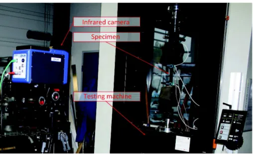
corresponding to the fiber direction. 3.2. Experimental setup

The experimental setup is shown inFig. 1. Tensile tests are per-formed with a 100 kN electromechanical testing machine

Table 1

Properties of the carbon/epoxy laminated composite and of its constituents (CES: data software Granta CES

selector).

Properties Units Values References

Compos. density q [kg m$3_{] 1449 Measured}

Compos. fiber vol fraction ff – 0.60 Hexcel

Compos. specific heat C [J/kg/K] 1000 CES Compos. time decrement s [s] 4.7 Measured Compos. thermal expansion aLðlongÞ (&10$5₎ [K$1_] $0.12 CES aTðtransÞ 3.40 Fiber thermal conductivity kL fðlong [W/m/K] 9.4 Toray kTf ðtransÞ 1.6 Matrix thermal conductivity km [W/m/K] 0.4 CES

INSTRON

5500R. These tests are performed at ambient tempera-ture with loading speed conventionally equal to 2 mm per min (0 ) and 1 mm per min (90 ). To check the reproducibility of the response, three specimens are considered for each loading direction.

During the tests, a thermal acquisition is carried out on one face of the sample with a FLIR

Titanium SC7000 retrofitted camera (InSb sensors, focal plane array of 320 256 pixels, thermal resolution of around 25 mK). Numerous acquisition parameters are selected up, the main ones being: the emissivity of the sample (0.98 for carbon fiber laminate), the sampling frequency (fs¼ 150 Hz) and the distance between the lens and the specimen

that leads to a spatial resolution smaller than 0.7 mm. Automatic calibration, control of the camera and data recording are done by Altair

software which is associated to the camera. Thermal images recorded by the infrared camera during the tensile tests thus capture the temporal and spatial dependency of the digitized temperature T. Altair

software allows to study a specific area of the sample. The size of studied area is of 218 36 pixels (respec-tively 154 33 pixels) with a pixel size of around 0.43 mm (resp. 0.68 mm) for 0 (resp. 90 ) tests. In agreement with assumptions considered inSection 2.1, the analysis is done on temperature vari-ation h obtained by subtracting to each measured thermal data T the average of the ten first frames corresponding to the reference temperature field T0.

4. Identification of a filtering process

Eq. (3)provides an estimation of the heat source fields from time and spatial derivatives of the thermal field. Since thermal measurements are discrete and strongly affected by noise pertur-bations resulting for instance from environmental disturbances, measurement devices and/or quantization, a data processing is necessary to obtain a relevant interpretation of measurements. 4.1. Methodology

The aim of the data processing is to reduce time and spatial noises amplitude while keeping useful information. As derivative process may be seen as a first order high pass filter, low pass filter-ing methods at least of first order in time domain and second order in spatial domain should be considered to clear undesired effects of

derivatives. Several filtering methods studied in the literature [11,13]have been investigated: linear filters of kind unweighted average (time and spatial moving average), linear filters of kind weighted average (Finite Impulse Response and Infinite Impulse Response), polynomial smoothing obtained using least-squares polynomial approximation, nonlinear filter (spatial-median filter with median value taken on a 3 3 pixels square).

Each term of the left-hand side of Eq.(3) has been analyzed separately. First, thermal variation h along time and its derivative _h have been studied. The determination of the temporal term _h has been performed with the numerical left derivation to keep high dynamic of useful signal observed in our case and to ensure causal-ity of processing. For the analysis of second-order partial deriva-tives according to space variables entering the spatial conduction laplacian term di

v

ð#k $ grad hÞ, central derivation commonly used

in signal processing has been applied. The characterization of the data processing has been addressed regarding two issues of the filtering efficiency. First, temporal efficiency has been studied through variations of the temperature on two pixels, the first one subjected to a strong damage during the test and the second one subjected to a low one. Then, we have investigated the spatial efficiency through variations of the temperature along a pixel line and along a pixel column at two instants (two frames), the first one subjected to a strong damage and the second one subjected to environmental noise (frame close to the beginning of the test). Such a work has been carried out with Matlab

software. 4.2. Evaluation and results

Since there is no theoretical signal that could be used as a refer-ence, several features of processed signals have been compared:

& Graphical plots of the original and filtered signals and their derivatives to give a first overview of the filtering efficiency. & Graphical plots of the Fourier Transform modulus of the original

and filtered signals and their derivatives to provide informa-tions about the original signal amplitude attenuainforma-tions along frequency.

& Pearson product-moment correlation coefficient to indicate the correlation degree between the original and filtered variables; this coefficient is between #1 (anticorrelation) and +1 (exact correlation), 0 corresponding to independent variables[15].

Standard deviation of the original and filtered signals on a noisy area in order to evaluate pure noise attenuation.

Standard deviation between specific points of the original and filtered curves to evaluate the preservation of the useful signal. As an illustration, a comparison of the efficiency of filtering methods is done on the estimation of the temporal derivative _hf

of the filtered temperature variation hf: Fig. 2a (respectively

Fig. 2b) provides the relative variation of original and filtered sig-nals standard deviations for the analysis of pure noise (resp. useful signal) attenuation andFig. 2c the value of the Pearson product-moment coefficient for each method. Therefore the best compro-mise corresponds to a high value inFig. 2a and c associated with a low value inFig. 2b. InFig. 3is also depicted the influence on the spatial and temporal evolution of the temperature.

It appears that the 3 ! 3 pixels spatial-median filter provides in our case the best results: it decreases the amplitude of noise (Figs. 2a and 3a), keeps the significant features of the signal (Figs. 2b and3b) and leads to an optimal correlation according to the Pearson product-moment correlation coefficient (Fig. 2c). The FIR low pass filter using Hamming window and the spatial 9 pixels (3 ! 3 pixels square) moving average also give interesting results. Yet, the former induces important delays and is not as effective on noise reduction (seeFig. 2a) and the latter tends to reduce the amplitude of the useful signal (seeFig. 2b). It has been noticed also that no temporal filtering is needed when using 3 ! 3 pixels median-filter on spatial temperature variation. Indeed, temporal dynamics of temperature is relatively slow regarding time sam-pling frequency (f_s¼ 150 Hz), so an efficient spatial filter naturally induces temporal filtering. It was also found that filtering on the derived terms is needless due to the satisfactory reduction of noise on the thermal fields with the spatial-median filter.

5. Estimation of the effective conductivity tensor by homogenization

As underlined in the Introduction, existing works often deal with isotropic materials for which the conductivity tensor is such that k ¼ k I with k a scalar value and I the second-order identity tensor. In our case, a transversely isotropic thermal conductivity tensor k needs to be considered to account for the oriented thermal conduction of studied composites. In view of the lack of experi-mental data, this section intends to determine such intrinsic data of the material by means of a homogenization scheme. Considering adequate conditions for the problem, such a method makes it possible to establish the effective properties of heterogeneous materials from their microstructural features [16]. Precisely, following developments are based on the strong analogy between well-known elasticity problems and conduction ones[17,18].

Let denoteXthe volume of the Representative Volume Element (RVE) of the heterogeneous material, @Xits outer boundary and n the outward unit normal to @X. The macroscopic temperature gradient G can be defined as the mean temperature on the bound-ary @X. From the divergence theorem, one can demonstrate that the macroscopic temperature gradient G corresponds to the average value of its microscopic corresponding quantity g:

G ¼1

X

Z @X TðzÞ nðzÞ dS ¼1

X

Z X gðzÞ dV ¼ hgi ð7Þ

where TðzÞ and gðzÞ ¼ grad TðzÞ denote respectively the local tem-perature and the local temtem-perature gradient for any point z of X. On the other hand, the macroscopic heat flux Q can be defined as the mean value of the external heat density on the boundary @X. Under stationary conditions (equivalent to usual equilibrium condi-tions of elasticity problems), one has di

v

q ¼ 0 and the divergence

theorem shows again that the macroscopic heat flux Q corresponds to the mean value of the local heat flux q:

Q ¼1

X

Z @X qðzÞ # nðzÞ z dS ¼1

X

Z X qðzÞ dV ¼ hqi ð8Þ

The RVE studied here is the laminated specimen itself including two phases (epoxy matrix and carbon fibers,Fig. 4), that can be considered as statistically homogeneous in regards to the fiber dimension. Spatial distribution of fibers is random, the matrix is continuous and interfaces are assumed to be perfect. Also, the material exhibits a ’matrix-inclusion’ morphology since fibers have the same shape, orientation and thermal behavior. Precisely, homogeneous constituents locally follow the Fourier linear thermal law. If the matrix can be considered as isotropic, fibers exhibit a transversely isotropic behavior around their unit axis x1. The local conductivity tensor is thus such that:

Fig. 3. Influence of two filtering methods on the temperature variation (0 sample).

Fig. 4. Representative Volume Element of the transversely isotropic composite considered; ðx1; x2; x3Þ forms an orthonormal basis.

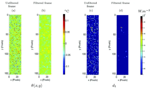
Fig. 5. Influence of the spatial-median filtering on the temperature variation field and on the associated mechanical dissipation field (90 sample, t ¼ tbt& 4dt with tbtthe

kðzÞ ¼ km¼ kmI;

8

z 2

X

m kf¼ k L fx1% x1þ k T fðI ' x1% x1Þ;

8

z 2

X

f ( ð9Þ

where kmdenotes the matrix conductivity, kLf (respectively k T f) the

fiber conductivity in the longitudinal (resp. transversal) direction and Xm (resp. Xf) the matrix (resp. fiber) volume such that

Xm[Xf ¼XandXm\Xf¼ £.

A uniform homogeneous macroscopic thermal gradient G is imposed at the outer boundary @Xof the RVE. Assuming an initial natural state, the superposition principle allows to relate local and macroscopic thermal gradients as follows:

gðzÞ ¼ AðzÞ # G;

8

z 2

X

ð10Þ

Second-order tensor A is called the concentration tensor and satis-fies hAi ¼ I to ensure the consistency condition(7). For homoge-neous constituents, the effective thermal conductivity of the composite khom that links overall quantities (Q ¼ (khom# G) comes

to the following simplified form[19,20]:

khom¼ X r frkr# hAir ð11Þ with fr¼Xr_X ! "

r¼ m;ff g the volume fraction of each phase and

h:ir¼Xr1 R

Xr: dV the average value on the phase r. Average

concen-tration tensor hAir provides then the average thermal gradient on

the r phase (hgir¼ hAir# G). Introducing the condition(7), Eq.(11)

comes to:

khom¼ kmþ ffðkf( kmÞ # hAif ð12Þ Works on the single-inhomogeneity problem, initiated by Eshelby in elasticity [21] and extended to thermoelasticity ([22–24] for example), provide solutions to derive estimations of hAif. In the

pre-sent context of an unidirectional composite with high carbon fiber volume fraction, the scheme proposed by Mori and Tanaka [25] has been choosen as it generally provides a good adequation with experimental results and finite element simulations. Moreover, it accounts in some way for the interactions between constituents. Accordingly, the concentration tensor of fibers writes:

hAif ¼ A f m# ð1 ( ffÞ I þ ffA f m h i(1 ð13Þ where Amf ¼ I þ S I E# ðkmÞ(1# ðkf( kmÞ h i(1 ð14Þ

The second-order depolarization tensor SI

E (the so-called Eshelby

tensor of elastic problems) depends on the shape and orientation of inclusions[18]. Since carbon fibers are modeled as an infinite

cylindrical inclusion of axis x1with circular section (Fig. 4), one has

[23,26]:

SIE¼ 1

2ðI " x1# x1Þ ð15Þ

Relevant calculations give rise to the final expression of the effec-tive conductivity of the composite, namely:

khom¼ k L homx1# x1þ k T homðI " x1# x1Þ ð16Þ with kLhom¼ ð1 " ffÞ kmþ ffk L f; k T hom¼ km ð1 " ffÞ kmþ ð1 þ ffÞ k T f ð1 þ ffÞ kmþ ð1 " ffÞ k T f ð17Þ

In agreement with the cylindrical geometry of fibers and their transversely isotropic behavior around the same axis, the composite exhibits also a transversely isotropic behavior around x1. Note also

that the effective longitudinal conductivity kL_homcorresponds to the classical law of mixtures and, more generally, that results are similar to those obtained with self-consistent formula[27,28]. Including data ofTable 1, numerical application leads to kLhom¼ 5; 80 W/m/K

and kThom¼ 0; 85 W/m/K, which confirms the preferential conduction

of the composite along its longitudinal direction.

6. Results and discussion

In a first step,Fig. 5intends to illustrate the influence of the spatial-median filter on the field data. The two first pictures show respectively the unfiltered (5a) and filtered (5b) temperature variation fields h of the whole sample at a specific instant of the 90 test, namely at t ¼ tbt" 4dt with tbt the breaking time and

dt ¼ 1=fs¼ 6:6 ms. This clearly demonstrates the interest of the

fil-tering process in avoiding spatial noise disturbances and in localiz-ing overheatlocaliz-ing (note that the reduction in time noise amplitude was previously illustrated inFig. 2). To highlight the influence of the filtering process on the source estimation, the mechanical heat source field d1 at the same instant has been established from

unfiltered (Fig. 5c) and filtered (Fig. 5d) temperature acquisitions. Global heat source st has been obtained from the procedure

detailed inSection 2and by using the effective thermal conductiv-ity tensor derived in Section 5. Material properties defined in Table 1have provided expressions of the stiffness C and thermal expansion

a

tensors (both transversely isotropic). The stress rate

_

r

given by the loading machine provides finally the mechanical

heat source d1 from the theoretical source sthe (Eqs.(3) and (6)).

Again, applying the spatial-median filter to the temperature data leads to a much more relevant interpretation of mechanical heat source that only reveals significant dissipative events. We can note also that overheating observed on temperature field (Fig. 5b) and most important source values (Fig. 5d) usually do not match. This reinforces the need to determine dissipation sources to get a more accurate indicator of damage.

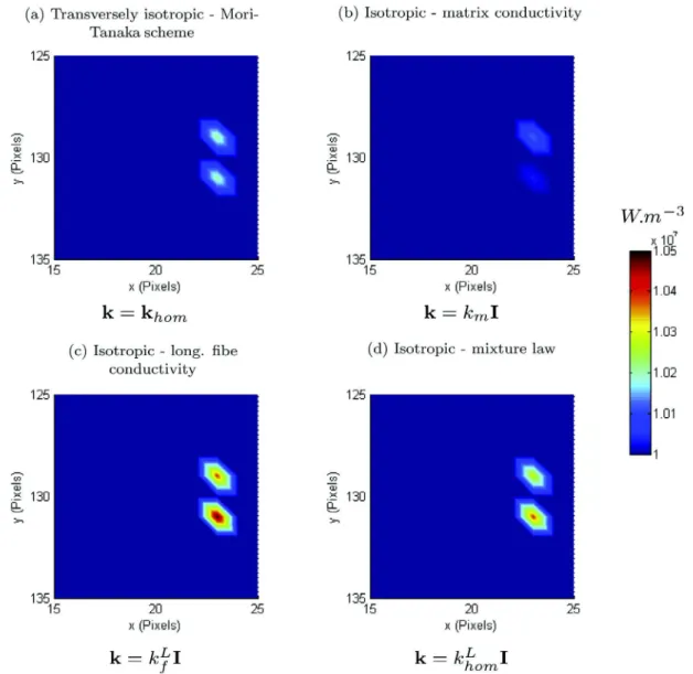
In a second step, we intend to investigate the influence of the material symmetry on the estimation of the mechanical dissipation field. For greater clearness, let focus on a local area (10 10 pixels) of the sample previously studied (90 test, t ¼ tbt" 4dt). Following

the procedure ofSection 2and working with filtered temperature, our aim is to compare the dissipation fields d1obtained when using

different expressions of the effective thermal conductivity tensor k. Graphical maps of Fig. 6 were thus obtained under different assumptions regarding the thermal conduction behavior. Precisely, Fig. 6a corresponds to the transversely isotropic conduction case studied inSection 5with conductivity tensor k given by Eq.(16). Three others figures were obtained with simplified representations based on an isotropic conduction behavior k ¼ kI:

# inFig. 6b, one uses the matrix conductivity (k ¼ km),

# in Fig. 6c, the longitudinal fiber conductivity is considered (k ¼ kLf),

# the last case shown in Fig. 6d deals with a law of mixture (k ¼ kLhom).

As shown by these pictures, the localization and intensity of the mechanical dissipation differ according to the considered material symmetry, and even differ between the three isotropic cases. Com-pared with the anisotropic case (Fig. 6a), using the matrix conduc-tivity (Fig. 6b) globally underestimates the heat source d1while the

longitudinal fiber value (Fig. 6c), and in a lesser extent the mixture law (Fig. 6d), overestimate it. These results are in agreement with

the order of magnitude of constituents conductivity properties (Table 1). Then, the two main sources obtained in the anisotropic case appear as quite equivalent in intensity (Fig. 6a), whereas isotropic conduction assumptions lead to distinct values. In the lat-ter case, the source of the top of pictureFig. 6b is higher than the bottom one, while reverse result is achieved inFigs. 6c and d. It is also worth noting that the mixture law case uses the same longitu-dinal conductivity value of k as the anisotropic case and differs only for its transverse component. Differences betweenFigs. 6a and d demonstrate that the anisotropic character of the thermal conduction clearly affects the mechanical dissipation sources. It is thus of main importance to introduce a physical representation of the thermal conduction behavior to get a relevant estimation of heat sources, and consequently to account for orientational effects involved in anisotropic materials. Such issue becomes even more crucial when the spatial conduction term di

v

ð"k % grad hÞ

represents the major part of the heat sources in the local heat equation. The homogenization approach used in this work to derive the effective thermal conductivity tensor offers then inter-esting perspectives to account for even more complex anisotropic situations.

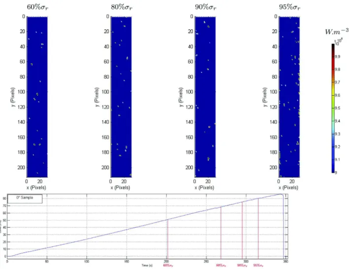
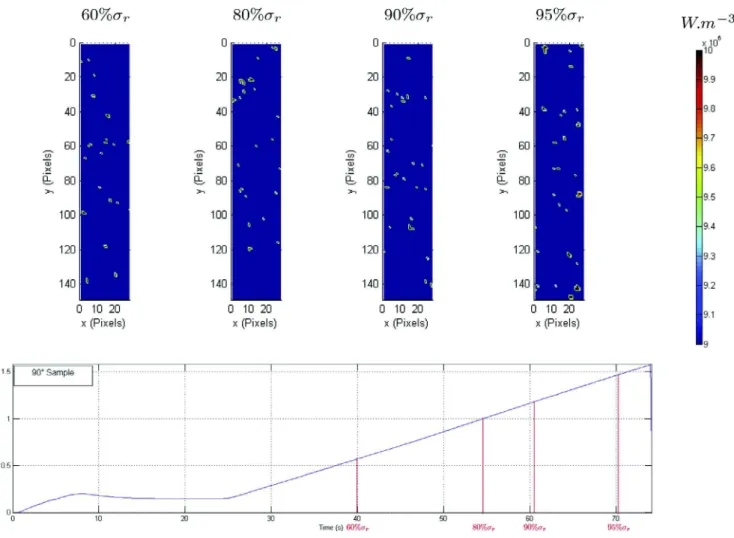
This last part finally illustrates some opportunities provided by the present work, specially for the damage analysis. Using the full methodology, including spatial-median filter and transversely isotropic conductivity tensor, we present the evolution of the mechanical dissipation during mechanical tests. InFig. 7 (respec-tivelyFig. 8) are depicted several maps of the mechanical dissipa-tion at different levels of the breaking stress

r

rfor the 0 (resp. 90)

loading direction. For both tests, we observe local dissipative phenomena, corresponding to local high amplitude mechanical dissipations, that are randomly distributed on specimen surfaces. This stands in agreement with the random location distribution of damage put in evidenced by tomography in woven carbon– epoxy laminates[4]. It is also worth noting that, for both axis and off-axis loads, mechanical dissipation d1at the beginning of

the test is of the same amplitude (around 107_{W m} 3_{) and that}

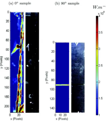
highest amplitude zones do not exhibit any preferential geometric shape or orientation. In contrast, dissipation behavior clearly dif-fers close to failure according to the loading direction. At 95% of the 0 yield stress, it can be observed an increase in the number of local dissipation events, whereas evolution of sources is much more progressive for the 90 test. The mode of dissipated energy can be related to damage mechanisms features and kinetics associ-ated to each loading configuration. 0 samples undergo fiber/ matrix debonding which suddenly accelerates at the end of the test leading to a macroscopic crack parallel to the axial direction. Mechanical dissipation field d1at breaking load has a very high

amplitude (maximum value greater than 4 ! 109_{W m} 3_{) and}

post-mortem observation illustrates such behavior (Fig. 9a). On the other hand, 90 samples exhibit a diffuse matrix cracking all along the test and failure corresponds to the development of the weakest defect in the direction orthogonal to the load. Fig. 9b corroborates the less brittle character of such failure mode with a lower level of dissipated energy d1 (maximum value of

2:8 ! 109W m 3_).

7. Conclusions

In this study, an original approach for estimating heat sources in anisotropic materials is presented. Input data are obtained from infrared thermographic measurements during axis and off-axis tensile tests on carbon–epoxy laminates. In order to determine the mechanical dissipations produced by the material considered,

a filtering method based on the use of a spatial-median filter has been developed. At the same time, the Mori–Tanaka homogeniza-tion approach has provided the effective transversely isotropic conductivity tensor of the composite material.

This work intends to provide a better interpretation of thermal measurements in anisotropic environment, leading to a much more accurate localization and characterization of dissipation sources. For instance, the application of the present methodology has allowed to demonstrate some correlations between most important dissipation events and acoustic emissions of high energy for carbon composites under tensile tests [29]. Moreover, the micromechanical contribution allows full perspectives to heat sources studies through the account of several parameters which may affect results, such as orientational aspects, spatial interac-tions between the constituents or damage evolution. Based on this approach, further works should now be conducted on various anisotropic material submitted to different loading configurations (specially off-axis loads) to improve the understanding of dissipa-tive phenomena and their modeling.

References

[1]Bruno L, Poggialini A. Optical methods in experimental mechanics. Opt Laser Eng 2007;45:537.

[2]Grédiac M. The use of full-field measurement method in composite material characterization: interests and limitations. Compos Part A-Appl Sci 2004;35:751–61.

[3]Chrysochoos A. Infrared thermography, a potential tool for analysing the material behaviour. Mec Ind 2002;3:3–14.

[4]Goidescu C, Welemane H, Garnier C, Fazzini M, Brault R, Péronnet E, Mistou S. Damage investigation in CFRP composites using full-field measurement techniques: combination of digital image stereo-correlation, infrared thermography and X-ray tomography. Compos Part B-Eng 2013;48:95–105. [5]Kordatos EZ, Dassios KG, Aggelis DG, Matikas TE. Rapid evaluation of the

fatigue limit in composites using infrared lock-in thermography and acoustic emission. Mech Res Commun 2013;54:14–20.

[6]Montesano J, Bougherara H, Fawaz Z. Application of infrared thermography for the characterization of damage in braided carbon fiber reinforced polymer matrix composites. Compos Part B-Eng 2014;60:137–43.

[7]Naderi M, Kahirdeh A, Khonsari MM. Dissipated thermal energy and damage evolution of glass/epoxy using infrared thermography and acoustic emission. Compos Part B 2012;43:1613–20.

[8]Benaarbia A, Chrysochoos A, Robert G. Kinetics of stored and dissipated energies associated with cyclic loadings of dry polyamide 6.6 specimens. Polym Test 2014;34:155–67.

[9]Berthel B, Watrisse B, Chrysochoos A, Galtier A. Thermographic analysis of fatigue dissipation properties of steel sheets. Strain 2007;43:273–9. [10]Boulanger T, Chrysochoos A, Mabru C, Galtier A. Calorimetric analysis of

dissipative and thermoelastic effects associated with the fatigue behavior of steels. Int J Fatigue 2004;26:221–9.

[11]Chrysochoos A, Louche H. An infrared image processing to analyse the calorific effects accompanying strain localisation. Int J Eng Sci 2000;38:1759–88. [12]Louche H, Chrysochoos A. Thermal and dissipative effects accompagnying

Lüders band propagation. Mater Sci+ 2001;307:15–22.

[13]Pastor ML, Balandraud X, Grédiac M, Robert JL. Applying infrared thermography to study the heating of 2024-T3 aluminium specimens under fatigue loading. Infrared Phys Technol 2008;51:505–15.

[14]Germain P, Nguyen QS, Suquet P. Continuum thermodynamics. J Appl Mech 1983;50:1010–20.

[15]Asuero AG, Sayago A, Gonzalez AG. The correlation coefficient: an overview. CRC Crit Rev Anal Chem 2006;36:41–59.

[16]Dormieux L, Kondo D, Ulm FJ. Microporomechanics. Chichester: Wiley & Sons; 2006.

[17]Norris A. On the correspondence between poroelasticity and thermoelasticity. J Appl Phys 1992;71:1138–41.

[18]Torquato S. Random heterogeneous materials. Microstructure and macroscopic properties. New York: Springer Science + Business Media; 2002. [19]Gruescu C, Giraud A, Homand F, Kondo D, Do DP. Effective thermal conductivity of partially saturated porous rocks. Int J Solids Struct 2007;44:811–33.

[20]Muliana AH, Kim JS. A two-scale homogenization framework for nonlinear effective thermal conductivity of laminated composites. Acta Mech 2010;212:319–47.

[21]Eshelby JD. The determination of the elastic field of an ellipsoidal inclusion and related problems. Proc Roy Soc Lond A Math 1957;A 421:376–96.

[22]Berryman JG. Generalization of Eshelby’s formula for a single ellipsoidal elastic inclusion to poroelasticity and thermoelasticity. Phys Rev Lett 1997; 79:1142–5.

Fig. 9. Mechanical dissipation field d1and post-mortem observation for 0 and 90

[23]Carslaw JC, Jaeger HS. Conduction of heat in solids. Oxford: Oxford University Press; 1959.

[24]Levin V, Alvarez-Tostado JM. Eshelby’s formula for an ellipsoidal elastic inclusion in anisotropic poroelasticity and thermoelasticity. Int J Fract 2003;119:L79–82.

[25]Mori T, Tanaka K. Average stress in matrix and average elastic energy of materials with misfitting inclusions. Acta Metall 1973;21:571–4.

[26]Hatta H, Taya M. Equivalent inclusion method for steady state heat conduction in composites. Int J Eng Sci 1986;24:1159–72.

[27]Lee JK. Prediction of thermal conductivities of laminated composites using penny-shaped fillers. J Mech Sci Technol 2008;22:2481–8.

[28]Rolfes R, Hammerschmidt U. Transverse thermal conductivity of CFRP laminates: a numerical and experimental validation of approximation formulae. Compos Sci Technol 1995;54:45–54.

[29] Munoz V, Valès B, Perrin M, Pastor ML, Welemane H, Cantarel A, Karama M. Damage detection in CFRP by coupling acoustic emission and infrared thermography. Compos Part B-Eng, in press, http://dx.doi.org/10.1016/ j.compositesb.2015.09.011.