HAL Id: hal-01434501
https://hal.archives-ouvertes.fr/hal-01434501
Submitted on 29 Mar 2017
HAL is a multi-disciplinary open access
archive for the deposit and dissemination of
sci-entific research documents, whether they are
pub-lished or not. The documents may come from
teaching and research institutions in France or
abroad, or from public or private research centers.
L’archive ouverte pluridisciplinaire HAL, est
destinée au dépôt et à la diffusion de documents
scientifiques de niveau recherche, publiés ou non,
émanant des établissements d’enseignement et de
recherche français ou étrangers, des laboratoires
publics ou privés.
Frédéric Bimbot, Jean-François Bonastre, Corinne Fredouille, Guillaume
Gravier, Ivan Magrin-Chagnolleau, Sylvain Meignier, Teva Merlin, Javier
Ortega-García, Dijana Petrovska-Delacrétaz, Douglas Reynolds
To cite this version:
Frédéric Bimbot, Jean-François Bonastre, Corinne Fredouille, Guillaume Gravier, Ivan
Magrin-Chagnolleau, et al..
A Tutorial on Text-Independent Speaker Verification.
EURASIP
Journal on Advances in Signal Processing, SpringerOpen, 2004, 2004 (4), pp.430 - 451.
�10.1155/S1110865704310024�. �hal-01434501�
A Tutorial on Text-Independent Speaker Verification
Fr ´ed ´eric Bimbot,1Jean-Franc¸ois Bonastre,2Corinne Fredouille,2Guillaume Gravier,1 Ivan Magrin-Chagnolleau,3Sylvain Meignier,2Teva Merlin,2Javier Ortega-Garc´ıa,4 Dijana Petrovska-Delacr ´etaz,5and Douglas A. Reynolds6
1IRISA, INRIA & CNRS, 35042 Rennes Cedex, France Emails:[email protected];[email protected]
2LIA, University of Avignon, 84911 Avignon Cedex 9, France
Emails:[email protected];[email protected];
[email protected];[email protected]
3Laboratoire Dynamique du Langage, CNRS, 69369 Lyon Cedex 07, France Email:[email protected]
4ATVS, Universidad Polit´ecnica de Madrid, 28040 Madrid, Spain Email:[email protected]
5DIVA Laboratory, Informatics Department, Fribourg University, CH-1700 Fribourg, Switzerland Email:[email protected]
6Lincoln Laboratory, Massachusetts Institute of Technology, Cambridge, MA 02420-9108, USA Email:[email protected]
Received 2 December 2002; Revised 8 August 2003
This paper presents an overview of a state-of-the-art text-independent speaker verification system. First, an introduction proposes a modular scheme of the training and test phases of a speaker verification system. Then, the most commonly speech parameteriza-tion used in speaker verificaparameteriza-tion, namely, cepstral analysis, is detailed. Gaussian mixture modeling, which is the speaker modeling technique used in most systems, is then explained. A few speaker modeling alternatives, namely, neural networks and support vector machines, are mentioned. Normalization of scores is then explained, as this is a very important step to deal with real-world data. The evaluation of a speaker verification system is then detailed, and the detection error trade-off (DET) curve is explained. Several extensions of speaker verification are then enumerated, including speaker tracking and segmentation by speakers. Then, some applications of speaker verification are proposed, including on-site applications, remote applications, applications relative to structuring audio information, and games. Issues concerning the forensic area are then recalled, as we believe it is very important to inform people about the actual performance and limitations of speaker verification systems. This paper concludes by giving a few research trends in speaker verification for the next couple of years.
Keywords and phrases: speaker verification, text-independent, cepstral analysis, Gaussian mixture modeling.
1. INTRODUCTION
Numerous measurements and signals have been proposed and investigated for use in biometric recognition systems. Among the most popular measurements are fingerprint, face, and voice. While each has pros and cons relative to accuracy and deployment, there are two main factors that have made voice a compelling biometric. First, speech is a natural sig-nal to produce that is not considered threatening by users to provide. In many applications, speech may be the main (or only, e.g., telephone transactions) modality, so users do not consider providing a speech sample for authentication
as a separate or intrusive step. Second, the telephone sys-tem provides a ubiquitous, familiar network of sensors for obtaining and delivering the speech signal. For telephone-based applications, there is no need for special signal trans-ducers or networks to be installed at application access points since a cell phone gives one access almost anywhere. Even for non-telephone applications, sound cards and microphones are low-cost and readily available. Additionally, the speaker recognition area has a long and rich scientific basis with over 30 years of research, development, and evaluations.
Over the last decade, speaker recognition technology has made its debut in several commercial products. The specific
Speaker model Statistical modeling module Speech parameters Speech parameterization module Speech data from a given speaker
Figure 1: Modular representation of the training phase of a speaker verification system.
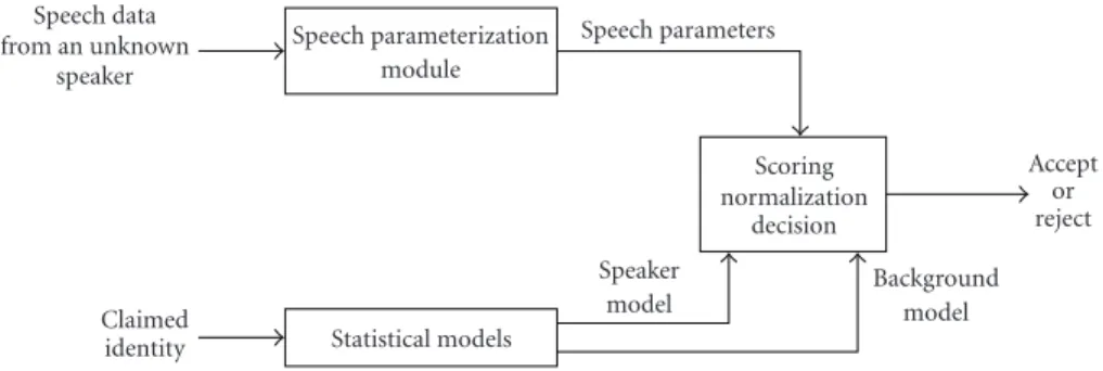
Background model Speaker model Statistical models Claimed identity Accept or reject Scoring normalization decision Speech parameters Speech parameterization module Speech data from an unknown speaker
Figure 2: Modular representation of the test phase of a speaker verification system.
recognition task addressed in commercial systems is that of verification or detection (determining whether an un-known voice is from a particular enrolled speaker) rather than identification (associating an unknown voice with one from a set of enrolled speakers). Most deployed applications are based on scenarios with cooperative users speaking fixed digit string passwords or repeating prompted phrases from a small vocabulary. These generally employ what is known as text-dependent or text-constrained systems. Such constraints are quite reasonable and can greatly improve the accuracy of a system; however, there are cases when such constraints can be cumbersome or impossible to enforce. An example of this is background verification where a speaker is verified behind the scene as he/she conducts some other speech interactions. For cases like this, a more flexible recognition system able to operate without explicit user cooperation and independent of the spoken utterance (called text-independent mode) is needed. This paper focuses on the technologies behind these text-independent speaker verification systems.
A speaker verification system is composed of two distinct phases, a training phase and a test phase. Each of them can be seen as a succession of independent modules.Figure 1shows a modular representation of the training phase of a speaker verification system. The first step consists in extracting pa-rameters from the speech signal to obtain a representation suitable for statistical modeling as such models are exten-sively used in most state-of-the-art speaker verification sys-tems. This step is described in Section 2. The second step consists in obtaining a statistical model from the parame-ters. This step is described inSection 3. This training scheme is also applied to the training of a background model (see Section 3).
Figure 2shows a modular representation of the test phase of a speaker verification system. The entries of the system are a claimed identity and the speech samples pronounced by an unknown speaker. The purpose of a speaker verification
system is to verify if the speech samples correspond to the claimed identity. First, speech parameters are extracted from the speech signal using exactly the same module as for the training phase (seeSection 2). Then, the speaker model cor-responding to the claimed identity and a background model are extracted from the set of statistical models calculated during the training phase. Finally, using the speech param-eters extracted and the two statistical models, the last mod-ule computes some scores, normalizes them, and makes an acceptance or a rejection decision (seeSection 4). The nor-malization step requires some score distributions to be esti-mated during the training phase or/and the test phase (see the details inSection 4).
Finally, a speaker verification system can be text-dependent or text-intext-dependent. In the former case, there is some constraint on the type of utterance that users of the system can pronounce (for instance, a fixed password or cer-tain words in any order, etc.). In the latter case, users can say whatever they want. This paper describes state-of-the-art text-independent speaker verification systems.
The outline of the paper is the following. Section 2 presents the most commonly used speech parameterization techniques in speaker verification systems, namely, cepstral analysis. Statistical modeling is detailed inSection 3, includ-ing an extensive presentation of Gaussian mixture eling (GMM) and the mention of several speaker mod-eling alternatives like neural networks and support vector machines (SVMs).Section 4explains how normalization is used.Section 5shows how to evaluate a speaker verification system. In Section 6, several extensions of speaker verifica-tion are presented, namely, speaker tracking and speaker seg-mentation.Section 7gives a few applications of speaker veri-fication.Section 8details specific problems relative to the use of speaker verification in the forensic area. Finally,Section 9 concludes this work and gives some future research direc-tions.
Cepstral vectors Cepstral transform Spectral vectors 20∗Log Filterbank | | FFT Windowing Pre-emphasis Speech signal
Figure 3: Modular representation of a filterbank-based cepstral parameterization.
2. SPEECH PARAMETERIZATION
Speech parameterization consists in transforming the speech signal to a set of feature vectors. The aim of this transforma-tion is to obtain a new representatransforma-tion which is more com-pact, less redundant, and more suitable for statistical mod-eling and the calculation of a distance or any other kind of score. Most of the speech parameterizations used in speaker verification systems relies on a cepstral representation of speech.
2.1. Filterbank-based cepstral parameters
Figure 3 shows a modular representation of a filterbank-based cepstral representation.
The speech signal is first preemphasized, that is, a filter is applied to it. The goal of this filter is to enhance the high frequencies of the spectrum, which are generally reduced by the speech production process. The preemphasized signal is obtained by applying the following filter:
xp(t)=x(t)−a·x(t−1). (1) Values of a are generally taken in the interval [0.95, 0.98]. This filter is not always applied, and some people prefer not to preemphasize the signal before processing it. There is no definitive answer to this topic but empirical experimentation. The analysis of the speech signal is done locally by the ap-plication of a window whose duration in time is shorter than the whole signal. This window is first applied to the begin-ning of the signal, then moved further and so on until the end of the signal is reached. Each application of the window to a portion of the speech signal provides a spectral vector (after the application of an FFT—see below). Two quantities have to be set: the length of the window and the shift between two consecutive windows. For the length of the window, two val-ues are most often used: 20 milliseconds and 30 milliseconds. These values correspond to the average duration which al-lows the stationary assumption to be true. For the delay, the value is chosen in order to have an overlap between two con-secutive windows; 10 milliseconds is very often used. Once these two quantities have been chosen, one can decide which window to use. The Hamming and the Hanning windows are the most used in speaker recognition. One usually uses a Hamming window or a Hanning window rather than a rectangular window to taper the original signal on the sides and thus reduce the side effects. In the Fourier domain, there is a convolution between the Fourier transform of the por-tion of the signal under considerapor-tion and the Fourier trans-form of the window. The Hamming window and the
Han-ning window are much more selective than the rectangular window.
Once the speech signal has been windowed, and possibly preemphasized, its fast Fourier transform (FFT) is calculated. There are numerous algorithms of FFT (see, for instance, [1, 2]).
Once an FFT algorithm has been chosen, the only param-eter to fix for the FFT calculation is the number of points for the calculation itself. This number N is usually a power of 2 which is greater than the number of points in the window, classically 512.
Finally, the modulus of the FFT is extracted and a power spectrum is obtained, sampled over 512 points. The spec-trum is symmetric and only half of these points are really useful. Therefore, only the first half of it is kept, resulting in a spectrum composed of 256 points.
The spectrum presents a lot of fluctuations, and we are usually not interested in all the details of them. Only the en-velope of the spectrum is of interest. Another reason for the smoothing of the spectrum is the reduction of the size of the spectral vectors. To realize this smoothing and get the enve-lope of the spectrum, we multiply the spectrum previously obtained by a filterbank. A filterbank is a series of band-pass frequency filters which are multiplied one by one with the spectrum in order to get an average value in a particu-lar frequency band. The filterbank is defined by the shape of the filters and by their frequency localization (left frequency, central frequency, and right frequency). Filters can be trian-gular, or have other shapes, and they can be differently lo-cated on the frequency scale. In particular, some authors use the Bark/Mel scale for the frequency localization of the fil-ters. This scale is an auditory scale which is similar to the fre-quency scale of the human ear. The localization of the central frequencies of the filters is given by
fMEL=1000·log
!
1 + fLIN/1000"
log 2 . (2)
Finally, we take the log of this spectral envelope and mul-tiply each coefficient by 20 in order to obtain the spectral en-velope in dB. At the stage of the processing, we obtain spec-tral vectors.
An additional transform, called the cosine discrete trans-form, is usually applied to the spectral vectors in speech pro-cessing and yields cepstral coefficients [2,3,4]:
cn= K # k=1 Sk·cos $ n % k−12 &π K ' , n=1, 2, . . . , L, (3)
Cepstral vectors Cepstral transform LPC vectors LPC algorithm Preemphasis Windowing Speech signal
Figure 4: Modular representation of an LPC-based cepstral parameterization.
where K is the number of log-spectral coefficients calcu-lated previously, Skare the log-spectral coefficients, and L is the number of cepstral coefficients that we want to calculate (L ≤K). We finally obtain cepstral vectors for each analysis
window.
2.2. LPC-based cepstral parameters
Figure 4 shows a modular representation of an LPC-based cepstral representation.
The LPC analysis is based on a linear model of speech production. The model usually used is an auto regressive moving average (ARMA) model, simplified in an auto re-gressive (AR) model. This modeling is detailed in particular in [5].
The speech production apparatus is usually described as a combination of four modules: (1) the glottal source, which can be seen as a train of impulses (for voiced sounds) or a white noise (for unvoiced sounds); (2) the vocal tract; (3) the nasal tract; and (4) the lips. Each of them can be repre-sented by a filter: a lowpass filter for the glottal source, an AR filter for the vocal tract, an ARMA filter for the nasal tract, and an MA filter for the lips. Globally, the speech production apparatus can therefore be represented by an ARMA filter. Characterizing the speech signal (usually a win-dowed portion of it) is equivalent to determining the coeffi-cients of the global filter. To simplify the resolution of this problem, the ARMA filter is often simplified in an AR fil-ter.
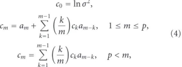
The principle of LPC analysis is to estimate the parame-ters of an AR filter on a windowed (preemphasized or not) portion of a speech signal. Then, the window is moved and a new estimation is calculated. For each window, a set of co-efficients (called predictive coco-efficients or LPC coco-efficients) is estimated (see [2,6] for the details of the various algo-rithms that can be used to estimate the LPC coefficients) and can be used as a parameter vector. Finally, a spectrum en-velope can be estimated for the current window from the predictive coefficients. But it is also possible to calculate cepstral coefficients directly from the LPC coefficients (see [6]): c0=ln σ2, cm=am+ m#−1 k=1 %k m & ckam−k, 1≤m≤p, cm= m#−1 k=1 %k m & ckam−k, p < m, (4)
where σ2is the gain term in the LPC model, a
mare the LPC
coefficients, and p is the number of LPC coefficients calcu-lated.
2.3. Centered and reduced vectors
Once the cepstral coefficients have been calculated, they can be centered, that is, the cepstral mean vector is subtracted from each cepstral vector. This operation is called cepstral mean subtraction (CMS) and is often used in speaker verifi-cation. The motivation for CMS is to remove from the cep-strum the contribution of slowly varying convolutive noises. The cepstral vectors can also be reduced, that is, the vari-ance is normalized to one component by component.
2.4. Dynamic information
After the cepstral coefficients have been calculated, and pos-sibly centered and reduced, we also incorporate in the vectors some dynamic information, that is, some information about the way these vectors vary in time. This is classically done by using the ∆ and ∆∆ parameters, which are polynomial ap-proximations of the first and second derivatives [7]:
∆cm= (l k=−lk·cm+k (l k=−l|k| , ∆∆cm= (l k=−lk2·cm+k (l k=−lk2 . (5)
2.5. Log energy and ∆ log energy
At this step, one can choose whether to incorporate the log energy and the ∆ log energy in the feature vectors or not. In practice, the former one is often discarded and the latter one is kept.
2.6. Discarding useless information
Once all the feature vectors have been calculated, a very im-portant last step is to decide which vectors are useful and which are not. One way of looking at the problem is to deter-mine vectors corresponding to speech portions of the signal versus those corresponding to silence or background noise. A way of doing it is to compute a bi-Gaussian model of the feature vector distribution. In that case, the Gaussian with the “lowest” mean corresponds to silence and background noise, and the Gaussian with the “highest” mean corre-sponds to speech portions. Then vectors having a higher like-lihood with the silence and background noise Gaussian are discarded. A similar approach is to compute a bi-Gaussian model of the log energy distribution of each speech segment and to apply the same principle.
3. STATISTICAL MODELING
3.1. Speaker verification via likelihood ratio detection
Given a segment of speech Y and a hypothesized speaker S, the task of speaker verification, also referred to as detection, is to determine if Y was spoken by S. An implicit assumption often used is that Y contains speech from only one speaker. Thus, the task is better termed singlespeaker verification. If there is no prior information that Y contains speech from a single speaker, the task becomes multispeaker detection. This paper is primarily concerned with the single-speaker verifica-tion task. Discussion of systems that handle the multispeaker detection task is presented in other papers [8].
The single-speaker detection task can be stated as a basic hypothesis test between two hypotheses:
H0: Y is from the hypothesized speaker S, H1: Y is not from the hypothesized speaker S.
The optimum test to decide between these two hypotheses is a likelihood ratio (LR) test1given by
p(Y|H0) p(Y|H1) ⎧ ⎨ ⎩ > θ, accept H0, < θ, accept H1, (6)
where p(Y|H0) is the probability density function for the hy-pothesis H0 evaluated for the observed speech segment Y, also referred to as the “likelihood” of the hypothesis H0 given the speech segment.2The likelihood function for H1 is
like-wise p(Y|H1). The decision threshold for accepting or reject-ing H0 is θ. One main goal in designreject-ing a speaker detection system is to determine techniques to compute values for the two likelihoods p(Y|H0) and p(Y|H1).
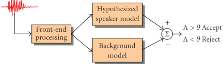
Figure 5shows the basic components found in speaker detection systems based on LRs. As discussed inSection 2, the role of the front-end processing is to extract from the speech signal features that convey speaker-dependent infor-mation. In addition, techniques to minimize confounding ef-fects from these features, such as linear filtering or noise, may be employed in the front-end processing. The output of this stage is typically a sequence of feature vectors representing the test segment X= {⃗x1, . . . ,⃗xT}, where⃗xtis a feature vector indexed at discrete time t ∈[1, 2, . . . , T]. There is no inher-ent constraint that features extracted at synchronous time in-stants be used; as an example, the overall speaking rate of an utterance could be used as a feature. These feature vectors are then used to compute the likelihoods of H0 and H1. Math-ematically, a model denoted by λhyp represents H0, which
characterizes the hypothesized speaker S in the feature space of⃗x. For example, one could assume that a Gaussian distribu-tion best represents the distribudistribu-tion of feature vectors for H0 so that λhypwould contain the mean vector and covariance
matrix parameters of the Gaussian distribution. The model
1Strictly speaking, the likelihood ratio test is only optimal when the
like-lihood functions are known exactly. In practice, this is rarely the case.
2p(A|B) is referred to as a likelihood when B is considered the
indepen-dent variable in the function.
Λ< θ Reject Λ> θ Accept Σ + − Hypothesized speaker model Background model Front-end processing
Figure 5: Likelihood-ratio-based speaker verification system.
λhyprepresents the alternative hypothesis, H1. The likelihood
ratio statistic is then p(X|λhyp)/ p(X|λhyp). Often, the
loga-rithm of this statistic is used giving the log LR Λ(X)=log p!X|λhyp"−log p
,
X|λhyp
-. (7) While the model for H0 is well defined and can be estimated using training speech from S, the model for λhypis less well defined since it potentially must represent the entire space of possible alternatives to the hypothesized speaker. Two main approaches have been taken for this alternative hypothesis modeling. The first approach is to use a set of other speaker models to cover the space of the alternative hypothesis. In various contexts, this set of other speakers has been called likelihood ratio sets [9], cohorts [9, 10], and background speakers [9,11]. Given a set of N background speaker models {λ1, . . . , λN}, the alternative hypothesis model is represented by
p,X|λhyp-= f!p!X|λ1", . . . , p!X|λN"", (8) where f (·) is some function, such as average or maximum, of the likelihood values from the background speaker set. The selection, size, and combination of the background speakers have been the subject of much research [9,10,11,12]. In gen-eral, it has been found that to obtain the best performance with this approach requires the use of speaker-specific back-ground speaker sets. This can be a drawback in applications using a large number of hypothesized speakers, each requir-ing their own background speaker set.
The second major approach to the alternative hypothesis modeling is to pool speech from several speakers and train a single model. Various terms for this single model are a gen-eral model [13], a world model, and a universal background model (UBM) [14]. Given a collection of speech samples from a large number of speakers representative of the popula-tion of speakers expected during verificapopula-tion, a single model
λbkg, is trained to represent the alternative hypothesis.
Re-search on this approach has focused on selection and com-position of the speakers and speech used to train the single model [15,16]. The main advantage of this approach is that a single speaker-independent model can be trained once for a particular task and then used for all hypothesized speak-ers in that task. It is also possible to use multiple background models tailored to specific sets of speakers [16,17]. The use of a single background model has become the predominate approach used in speaker verification systems.
3.2. Gaussian mixture models
An important step in the implementation of the above like-lihood ratio detector is the selection of the actual likelike-lihood function p(X|λ). The choice of this function is largely
depen-dent on the features being used as well as specifics of the ap-plication. For text-independent speaker recognition, where there is no prior knowledge of what the speaker will say, the most successful likelihood function has been GMMs. In text-dependent applications, where there is a strong prior knowl-edge of the spoken text, additional temporal knowlknowl-edge can be incorporated by using hidden Markov models (HMMs) for the likelihood functions. To date, however, the use of more complicated likelihood functions, such as those based on HMMs, have shown no advantage over GMMs for text-independent speaker detection tasks like in the NIST speaker recognition evaluations (SREs).
For a D-dimensional feature vector⃗x, the mixture density used for the likelihood function is defined as follows:
p!⃗x|λ"= M # i=1
wipi!⃗x". (9) The density is a weighted linear combination of M unimodal Gaussian densities pi(⃗x), each parameterized by a D×1 mean vector⃗µiand a D×D covariance matrix Σi:
pi!⃗x"= 1 (2π)D/2..Σi..1/2e
−(1/2)(⃗x−⃗µi)′Σi−1(⃗x−⃗µi). (10)
The mixture weights wi further satisfy the constraint (M
i=1wi = 1. Collectively, the parameters of the density model are denoted as λ=(wi,⃗µi, Σi), i=(1, . . . , M).
While the general model form supports full covariance matrices, that is, a covariance matrix with all its elements, typically only diagonal covariance matrices are used. This is done for three reasons. First, the density modeling of an
Mth-order full covariance GMM can equally well be achieved
using a larger-order diagonal covariance GMM.3 Second,
diagonal-matrix GMMs are more computationally efficient than full covariance GMMs for training since repeated inver-sions of a D×D matrix are not required. Third, empirically, it
has been observed that diagonal-matrix GMMs outperform full-matrix GMMs.
Given a collection of training vectors, maximum like-lihood model parameters are estimated using the iterative expectation-maximization (EM) algorithm [18]. The EM al-gorithm iteratively refines the GMM parameters to mono-tonically increase the likelihood of the estimated model for the observed feature vectors, that is, for iterations k and k +1,
p(X|λ(k+1)) ≥ p(X|λ(k)). Generally, five–ten iterations are
sufficient for parameter convergence. The EM equations for training a GMM can be found in the literature [18,19,20].
3GMMs with M > 1 using diagonal covariance matrices can model
dis-tributions of feature vectors with correlated elements. Only in the degenerate case of M=1 is the use of a diagonal covariance matrix incorrect for feature vectors with correlated elements.
Under the assumption of independent feature vectors, the log-likelihood of a model λ for a sequence of feature vec-tors X= {⃗x1, . . . ,⃗xT}is computed as follows:
log p(X|λ)= 1
T
# t
log p!⃗xt|λ", (11) where p(⃗xt|λ) is computed as in equation (9). Note that the average log-likelihood value is used so as to normalize out duration effects from the log-likelihood value. Also, since the incorrect assumption of independence is underestimat-ing the actual likelihood value with dependencies, scalunderestimat-ing by
T can be considered a rough compensation factor.
The GMM can be viewed as a hybrid between parametric and nonparametric density models. Like a parametric model, it has structure and parameters that control the behavior of the density in known ways, but without constraints that the data must be of a specific distribution type, such as Gaus-sian or Laplacian. Like a nonparametric model, the GMM has many degrees of freedom to allow arbitrary density mod-eling, without undue computation and storage demands. It can also be thought of as a single-state HMM with a Gaussian mixture observation density, or an ergodic Gaussian obser-vation HMM with fixed, equal transition probabilities. Here, the Gaussian components can be considered to be model-ing the underlymodel-ing broad phonetic sounds that characterize a person’s voice. A more detailed discussion of how GMMs apply to speaker modeling can be found elsewhere [21].
The advantages of using a GMM as the likelihood func-tion are that it is computafunc-tionally inexpensive, is based on a well-understood statistical model, and, for text-independent tasks, is insensitive to the temporal aspects of the speech, modeling only the underlying distribution of acoustic obser-vations from a speaker. The latter is also a disadvantage in that higher-levels of information about the speaker conveyed in the temporal speech signal are not used. The modeling and exploitation of these higher-levels of information may be where approaches based on speech recognition [22] produce benefits in the future. To date, however, these approaches (e.g., large vocabulary or phoneme recognizers) have basi-cally been used only as means to compute likelihood values, without explicit use of any higher-level information, such as speaker-dependent word usage or speaking style. Some re-cent work, however, has shown that high-level information can be successfully extracted and combined with acoustic scores from a GMM system for improved speaker verification performance [23,24].
3.3. Adapted GMM system
As discussed earlier, the dominant approach to background modeling is to use a single, speaker-independent background model to represent p(X|λhyp). Using a GMM as the
likeli-hood function, the background model is typically a large GMM trained to represent the speaker-independent distri-bution of features. Specifically, speech should be selected that reflects the expected alternative speech to be encoun-tered during recognition. This applies to the type and qual-ity of speech as well as the composition of speakers. For
example, in the NIST SRE single-speaker detection tests, it is known a priori that the speech comes from local and long-distance telephone calls, and that male hypothesized speak-ers will only be tested against male speech. In this case, we would train the UBM used for male tests using only male telephone speech. In the case where there is no prior knowl-edge of the gender composition of the alternative speakers, we would train using gender-independent speech. The GMM order for the background model is usually set between 512– 2048 mixtures depending on the data. Lower-order mixtures are often used when working with constrained speech (such as digits or fixed vocabulary), while 2048 mixtures are used when dealing with unconstrained speech (such as conversa-tional speech).
Other than these general guidelines and experimenta-tion, there is no objective measure to determine the right number of speakers or amount of speech to use in train-ing a background model. Empirically, from the NIST SRE, we have observed no performance loss using a background model trained with one hour of speech compared to a one trained using six hours of speech. In both cases, the training speech was extracted from the same speaker population.
For the speaker model, a single GMM can be trained us-ing the EM algorithm on the speaker’s enrollment data. The order of the speaker’s GMM will be highly dependent on the amount of enrollment speech, typically 64–256 mixtures. In another more successful approach, the speaker model is de-rived by adapting the parameters of the background model using the speaker’s training speech and a form of Bayesian adaptation or maximum a posteriori (MAP) estimation [25]. Unlike the standard approach of maximum likelihood train-ing of a model for the speaker, independently of the back-ground model, the basic idea in the adaptation approach is to derive the speaker’s model by updating the well-trained parameters in the background model via adaptation. This provides a tighter coupling between the speaker’s model and background model that not only produces better perfor-mance than decoupled models, but, as discussed later in this section, also allows for a fast-scoring technique. Like the EM algorithm, the adaptation is a two-step estimation process. The first step is identical to the “expectation” step of the EM algorithm, where estimates of the sufficient statistics4of
the speaker’s training data are computed for each mixture in the UBM. Unlike the second step of the EM algorithm, for adaptation, these “new” sufficient statistic estimates are then combined with the “old” sufficient statistics from the back-ground model mixture parameters using a data-dependent mixing coefficient. The data-dependent mixing coefficient is designed so that mixtures with high counts of data from the speaker rely more on the new sufficient statistics for final pa-rameter estimation, and mixtures with low counts of data from the speaker rely more on the old sufficient statistics for final parameter estimation.
4These are the basic statistics required to compute the desired
param-eters. For a GMM mixture, these are the count, and the first and second moments required to compute the mixture weight, mean and variance.
The specifics of the adaptation are as follows. Given a background model and training vectors from the hypothe-sized speaker, we first determine the probabilistic alignment of the training vectors into the background model mixture components. That is, for mixture i in the background model, we compute Pr!i|⃗xt"= wipi !⃗x t" (M j=1wjpj!⃗xt" . (12)
We then use Pr(i|⃗xt) and⃗xtto compute the sufficient statistics for the weight, mean, and variance parameters:5
ni= T # t=1 Pr!i|⃗xt", Ei!⃗x"=n1 i T # t=1 Pr!i|⃗xt"⃗xt, Ei!⃗x2"=n1 i T # t=1 Pr!i|⃗xt"⃗xt2. (13)
This is the same as the expectation step in the EM algorithm. Lastly, these new sufficient statistics from the training data are used to update the old background model sufficient statistics for mixture i to create the adapted parameters for mixture i with the equations
ˆ wi=/αini/T +!1−αi"wi0γ, ˆ⃗µi=αiEi!⃗x"+!1−αi"⃗µi, ˆ⃗σ2 i =αiEi!⃗x2"+!1−αi"!⃗σi2+⃗µi2 " −ˆ⃗µ2 i. (14)
The scale factor γ is computed over all adapted mixture weights to ensure they sum to unity. The adaptation coeffi-cient controlling the balance between old and new estimates is αiand is defined as follows:
αi=nni
i+ r, (15)
where r is a fixed “relevance” factor.
The parameter updating can be derived from the general MAP estimation equations for a GMM using constraints on the prior distribution described in Gauvain and Lee’s paper [25, Section V, equations (47) and (48)]. The parameter up-dating equation for the weight parameter, however, does not follow from the general MAP estimation equations.
Using a data-dependent adaptation coefficient allows mixture-dependent adaptation of parameters. If a mixture component has a low probabilistic count ni of new data, then αi → 0 causing the deemphasis of the new (poten-tially under-trained) parameters and the emphasis of the old (better trained) parameters. For mixture components with high probabilistic counts, αi →1 causing the use of the new speaker-dependent parameters. The relevance factor is a way
of controlling how much new data should be observed in a mixture before the new parameters begin replacing the old parameters. This approach should thus be robust to limited training data. This factor can also be made parameter de-pendent, but experiments have found that this provides little benefit. Empirically, it has been found that only adapting the mean vectors provides the best performance.
Published results [14] and NIST evaluation results from several sites strongly indicate that the GMM adaptation ap-proach provides superior performance over a decoupled sys-tem, where the speaker model is trained independently of the background model. One possible explanation for the improved performance is that the use of adapted models in the likelihood ratio is not affected by “unseen” acous-tic events in recognition speech. Loosely speaking, if one considers the background model as covering the space of speaker-independent, broad acoustic classes of speech sounds, then adaptation is the speaker-dependent “tuning” of those acoustic classes observed in the speaker’s train-ing speech. Mixture parameters for those acoustic classes not observed in the training speech are merely copied from the background model. This means that during recogni-tion, data from acoustic classes unseen in the speaker’s train-ing speech produce approximately zero log LR values that contribute evidence neither towards nor against the hy-pothesized speaker. Speaker models trained using only the speaker’s training speech will have low likelihood values for data from classes not observed in the training data thus pro-ducing low likelihood ratio values. While this is appropriate for speech not for the speaker, it clearly can cause incorrect values when the unseen data occurs in test speech from the speaker.
The adapted GMM approach also leads to a fast-scoring technique. Computing the log LR requires computing the likelihood for the speaker and background model for each feature vector, which can be computationally expensive for large mixture orders. However, the fact that the hypothesized speaker model was adapted from the background model al-lows a faster scoring method. This fast-scoring approach is based on two observed effects. The first is that when a large GMM is evaluated for a feature vector, only a few of the mix-tures contribute significantly to the likelihood value. This is because the GMM represents a distribution over a large space but a single vector will be near only a few components of the GMM. Thus likelihood values can be approximated very well using only the top C best scoring mixture components. The second observed effect is that the components of the adapted GMM retain a correspondence with the mixtures of the back-ground model so that vectors close to a particular mixture in the background model will also be close to the corresponding mixture in the speaker model.
Using these two effects, a fast-scoring procedure oper-ates as follows. For each feature vector, determine the top
C scoring mixtures in the background model and compute
background model likelihood using only these top C mix-tures. Next, score the vector against only the corresponding
C components in the adapted speaker model to evaluate the
speaker’s likelihood.
For a background model with M mixtures, this re-quires only M + C Gaussian computations per feature vector compared to 2M Gaussian computations for normal likeli-hood ratio evaluation. When there are multiple hypothesized speaker models for each test segment, the savings become even greater. Typically, a value of C=5 is used.
3.4. Alternative speaker modeling techniques
Another way to solve the classification problem for speaker verification systems is to use discrimination-based learning procedures such as artificial neural networks (ANN) [26,27] or SVMs [28]. As explained in [29,30], the main advantages of ANN include their discriminant-training power, a flexible architecture that permits easy use of contextual information, and weaker hypothesis about the statistical distributions. The main disadvantages are that their optimal structure has to be selected by trial-and-error procedures, the need to split the available train data in training and cross-validation sets, and the fact that the temporal structure of speech signals re-mains difficult to handle. They can be used as binary classi-fiers for speaker verification systems to separate the speaker and the nonspeaker classes as well as multicategory classifiers for speaker identification purposes. ANN have been used for speaker verification [31,32,33]. Among the different ANN architectures, multilayer perceptrons (MLP) are often used [6,34].
SVMs are an increasingly popular method used in speaker verifications systems. SVM classifiers are well suited to separate rather complex regions between two classes through an optimal, nonlinear decision boundary. The main problems are the search for the appropriate kernel function for a particular application and their inappropriateness to handle the temporal structure of the speech signals. There are also some recent studies [35] in order to adapt the SVM to the multicategory classification problem. The SVM were al-ready applied for speaker verification. In [23,36], the widely used speech feature vectors were used as the input training material for the SVM.
Generally speaking, the performance of speaker verifica-tion systems based on discriminaverifica-tion-based learning tech-niques can be tuned to obtain comparable performance to the state-of-the-art GMM, and in some special experimen-tal conditions, they could be tuned to outperform the GMM. It should be noted that, as explained earlier in this section, the tuning of a GMM baseline systems is not straightfor-ward, and different parameters such as the training method, the number of mixtures, and the amount of speech to use in training a background model have to be adjusted to the experimental conditions. Therefore, when comparing a new system to the classical GMM system, it is difficult to be sure that the baseline GMM used are comparable to the best per-forming ones.
Another recent alternative to solve the speaker verifica-tion problem is to combine GMM with SVMs. We are not going to give here an extensive study of all the experiments done [37,38,39], but we are rather going to illustrate the problem with one example meant to exploit together the GMM and SVM for speaker verification purposes. One of the
problems with the speaker verification is the score normal-ization (seeSection 4). Because SVM are well suited to deter-mine an optimal hyperplan separating data belonging to two classes, one way to use them for speaker verification is to sep-arate the likelihood client and nonclient values with an SVM. That was the idea implemented in [37], and an SVM was constructed to separate two classes, the clients from the im-postors. The GMM technique was used to construct the in-put feature representation for the SVM classifier. The speaker GMM models were built by adaptation of the background model. The GMM likelihood values for each frame and each Gaussian mixture were used as the input feature vector for the SVM. This combined GMM-SVM method gave slightly better results than the GMM method alone. Several points should be emphasized: the results were obtained on a sub-set of NIST’1999 speaker verification data, only the Znorm was tested, and neither the GMM nor the SVM parameters were thoroughly adjusted. The conclusion is that the results demonstrate the feasibility of this technique, but in order to fully exploit these two techniques, more work should be done.
4. NORMALIZATION
4.1. Aims of score normalization
The last step in speaker verification is the decision making. This process consists in comparing the likelihood resulting from the comparison between the claimed speaker model and the incoming speech signal with a decision threshold. If the likelihood is higher than the threshold, the claimed speaker will be accepted, else rejected.
The tuning of decision thresholds is very troublesome in speaker verification. If the choice of its numerical value remains an open issue in the domain (usually fixed empir-ically), its reliability cannot be ensured while the system is running. This uncertainty is mainly due to the score variabil-ity between trials, a fact well known in the domain.
This score variability comes from different sources. First, the nature of the enrollment material can vary between the speakers. The differences can also come from the phonetic content, the duration, the environment noise, as well as the quality of the speaker model training. Secondly, the pos-sible mismatch between enrollment data (used for speaker modeling) and test data is the main remaining problem in speaker recognition. Two main factors may contribute to this mismatch: the speaker him-/herself through the intraspeaker variability (variation in speaker voice due to emotion, health state, and age) and some environment condition changes in transmission channel, recording material, or acoustical en-vironment. On the other hand, the interspeaker variability (variation in voices between speakers), which is a particular issue in the case of speaker-independent threshold-based sys-tem, has to be also considered as a potential factor affecting the reliability of decision boundaries. Indeed, as this inters-peaker variability is not directly measurable, it is not straight-forward to protect the speaker verification system (through the decision making process) against all potential impostor
attacks. Lastly, as for the training material, the nature and the quality of test segments influence the value of the scores for client and impostor trials.
Score normalization has been introduced explicitly to cope with score variability and to make speaker-independent decision threshold tuning easier.
4.2. Expected behavior of score normalization
Score normalization techniques have been mainly derived from the study of Li and Porter [40]. In this paper, large variances had been observed from both distributions of client scores (intraspeaker scores) and impostor scores (in-terspeaker scores) during speaker verification tests. Based on these observations, the authors proposed solutions based on impostor score distribution normalization in order to reduce the overall score distribution variance (both client and im-postor distributions) of the speaker verification system. The basic of the normalization technique is to center the impos-tor score distribution by applying on each score generated by the speaker verification system the following normalization. Let Lλ(X) denote the score for speech signal X and speaker model λ. The normalized score 1Lλ(X) is then given as fol-lows:
1
Lλ(X)=Lλ(X)σ−µλ
λ , (16)
where µλand σλare the normalization parameters for speaker
λ. Those parameters need to be estimated.
The choice of normalizing the impostor score distribu-tion (as opposed to the client score distribudistribu-tion) was ini-tially guided by two facts. First, in real applications and for text-independent systems, it is easy to compute impostor score distributions using pseudo-impostors, but client distri-butions are rarely available. Secondly, impostor distribution represents the largest part of the score distribution variance. However, it would be interesting to study client score dis-tribution (and normalization), for example, in order to de-termine theoretically the decision threshold. Nevertheless, as seen previously, it is difficult to obtain the necessary data for real systems and only few current databases contain enough data to allow an accurate estimate of client score distribution.
4.3. Normalization techniques
Since the study of Li and Porter [40], various kinds of score normalization techniques have been proposed in the litera-ture. Some of them are briefly described in the following sec-tion.
World-model and cohort-based normalizations
This class of normalization techniques is a particular case: it relies more on the estimation of antispeaker hypothesis (“the target speaker does not pronounce the record”) in the Bayesian hypothesis test than on a normalization scheme. However, the effects of this kind of techniques on the dif-ferent score distributions are so close to the normalization method ones that we have to present here.
The first proposal came from Higgins et al. in 1991 [9], followed by Matsui and Furui in 1993 [41], for which the normalized scores take the form of a ratio of likelihoods as follows:
1
Lλ(X)=Lλ(X)
Lλ(X). (17) For both approaches, the likelihood Lλ(y) was estimated from a cohort of speaker models. In [9], the cohort of speak-ers (also denoted as a cohort of impostors) was chosen to be close to speaker λ. Conversely, in [41], the cohort of speakers included speaker λ. Nevertheless, both normaliza-tion schemes equally improve speaker verificanormaliza-tion perfor-mance.
In order to reduce the amount of computation, the co-hort of impostor models was replaced later with a unique model learned using the same data as the first ones. This idea is the basic of world-model normalization (the world model is also named “background model”) firstly introduced by Carey et al. [13]. Several works showed the interest in world-model-based normalization [14,17,42].
All the other normalizations discussed in this paper are applied on world-model normalized scores (commonly named likelihood ratio in the way of statistical approaches), that is,1Lλ(X)=Λλ(X).
Centered/reduced impostor distribution
This family of normalization techniques is the most used. It is directly derived from (16), where the scores are normalized by subtracting the mean and then dividing by the standard deviation, both estimated from the (pseudo)impostor score distribution. Different possibilities are available to compute the impostor score distribution.
Znorm
The zero normalization (Znorm) technique is directly de-rived from the work done in [40]. It has been massively used in speaker verification in the middle of the nineties. In prac-tice, a speaker model is tested against a set of speech sig-nals produced by some impostor, resulting in an impostor similarity score distribution. Speaker-dependent mean and variance—normalization parameters—are estimated from this distribution and applied (see (16) on similarity scores yielded by the speaker verification system when running. One of the advantages of Znorm is that the estimation of the normalization parameters can be performed offline during speaker model training.
Hnorm
By observing that, for telephone speech, most of the client speaker models respond differently according to the hand-set type used during testing data recording, Reynolds [43] had proposed a variant of Znorm technique, named hand-set normalization (Hnorm), to deal with handhand-set mismatch between training and testing.
Here, handset-dependent normalization parameters are estimated by testing each speaker model against
handset-dependent speech signals produced by impostors. During testing, the type of handset relating to the incoming speech signal determines the set of parameters to use for score nor-malization.
Tnorm
Still based on the estimate of mean and variance parameters to normalize impostor score distribution, test-normalization (Tnorm), proposed in [44], differs from Znorm by the use of impostor models instead of test speech signals. During testing, the incoming speech signal is classically compared with claimed speaker model as well as with a set of impos-tor models to estimate imposimpos-tor score distribution and nor-malization parameters consecutively. If Znorm is considered as a speaker-dependent normalization technique, Tnorm is a test-dependent one. As the same test utterance is used during both testing and normalization parameter estimate, Tnorm avoids a possible issue of Znorm based on a possible mismatch between test and normalization utterances. Con-versely, Tnorm has to be performed online during testing.
HTnorm
Based on the same observation as Hnorm, a variant of Tnorm has been proposed, named HTnorm, to deal with handset-type information. Here, handset-dependent nor-malization parameters are estimated by testing each incom-ing speech signal against handset-dependent impostor mod-els. During testing, the type of handset relating to the claimed speaker model determines the set of parameters to use for score normalization.
Cnorm
Cnorm was introduced by Reynolds during NIST 2002 speaker verification evaluation campaigns in order to deal with cellular data. Indeed, the new corpus (Switchboard cel-lular phase 2) is composed of recordings obtained using dif-ferent cellular phones corresponding to several unidentified handsets. To cope with this issue, Reynolds proposed a blind clustering of the normalization data followed by an Hnorm-like process using each cluster as a different handset.
This class of normalization methods offers some ad-vantages particularly in the framework of NIST evaluations (text independent speaker verification using long segments of speech—30 seconds in average for tests and 2 minutes for enrollment). First, both the method and the impostor dis-tribution model are simple, only based on mean and stan-dard deviation computation for a given speaker (even if Tnorm complicates the principle by the need of online pro-cessing). Secondly, the approach is well adapted to a text-independent task, with a large amount of data for enroll-ment. These two points allow to find easily pseudo-impostor data. It seems more difficult to find these data in the case of a user-password-based system, where the speaker chooses his password and repeats it three or four times during the enroll-ment phase only. Lastly, modeling only the impostor distri-bution is a good way to set a threshold according to the global false acceptance error and reflects the NIST scoring strategy.
For a commercial system, the level of false rejection is critical and the quality of the system is driven by the quality reached for the “worse” speakers (and not for the average).
Dnorm
Dnorm was proposed by Ben et al. in 2002 [45]. Dnorm deals with the problem of pseudo-impostor data availabil-ity by generating the data using the world model. A Monte Carlo-based method is applied to obtain a set of client and impostor data, using, respectively, client and world models. The normalized score is given by
1
Lλ(X)= Lλ(X)
KL2!λ, λ", (18)
where KL2(λ, λ) is the estimate of the symmetrized Kullback-Leibler distance between the client and world models. The estimation of the distance is done using Monte-Carlo gen-erated data. As for the previous normalizations, Dnorm is applied on likelihood ratio, computed using a world model.
Dnorm presents the advantage not to need any nor-malization data in addition to the world model. As Dnorm is a recent proposition, future developments will show if the method could be applied in different applications like password-based systems.
WMAP
WMAP is designed for multirecognizer systems. The tech-nique focuses on the meaning of the score and not only on normalization. WMAP, proposed by Fredouille et al. in 1999 [46], is based on the Bayesian decision framework. The orig-inality is to consider the two classical speaker recognitionhy-potheses in the score space and not in the acoustic space. The final score is the a posteriori probability to obtain the score given the target hypothesis:
WMAP!Lλ(X)"
= PTarget·p !
Lλ(X)|Target"
PTarget·p!Lλ(X)|Target"+ PImp·p!Lλ(X)|Imp", (19) where PTarget(resp., PImp) is the a priori probability of a
tar-get test (resp., an impostor test) and p(Lλ(X)|Target) (resp.,
p(Lλ(X)|Imp)) is the probability of score Lλ(X) given the hy-pothesis of a target test (resp., an impostor test).
The main advantage of the WMAP6 normalization is
to produce meaningful normalized score in the probability space. The scores take the quality of the recognizer directly into account, helping the system design in the case of multi-ple recognizer decision fusion.
The implementation proposed by Fredouille in 1999 used an empirically approach and nonparametric models for esti-mating the target and impostor score probabilities.
6The method is called WMAP as it is a maximum a posteriori approach
applied on likelihood ratio where the denominator is computed using a world model.
4.4. Discussion
Through the various experiments achieved on the use of nor-malization in speaker verification, different points may be highlighted. First of all, the use of prior information like the handset type or gender information during normalization parameter computation is relevant to improve performance (see [43] for experiments on Hnorm and [44] for experiment on HTnorm).
Secondly, HTnorm seems better than the other kind of normalization as shown during the 2001 and 2002 NIST evaluation campaigns. Unfortunately, HTnorm is also the most expensive in computational time and requires estimat-ing normalization parameters durestimat-ing testestimat-ing. The solution proposed in [45], Dnorm normalization, may be a promis-ing alternative since the computational time is significantly reduced and no impostor population is required to esti-mate normalization parameters. Currently, Dnorm performs as well as Znorm technique [45]. Further work is expected in order to integrate prior information like handset type to Dnorm and to make it comparable with Hnorm and HT-norm. WMAP technique exhibited interesting performance (same level as Znorm but without any knowledge about the real target speaker—normalization parameters are learned a priori using a separate set of speakers/tests). However, the technique seemed difficult to apply in a target speaker-dependent mode, since few speaker data are not sufficient to learn the normalization models. A solution could be to gen-erate data, as done in the Dnorm approach, to estimate the score models Target and Imp (impostor) directly from the models.
Finally, as shown during the 2001 and 2002 NIST evalu-ation campaigns, the combinevalu-ation of different kinds of nor-malization (e.g., HTnorm & Hnorm, Tnorm & Dnorm) may lead to improved speaker verification performance. It is in-teresting to note that each winning normalization combina-tion relies on the associacombina-tion between a “learning condicombina-tion” normalization (Znorm, Hnorm, and Dnorm) and a “test-based” normalization (HTnorm and Tnorm).
However, this behavior of current speaker verification systems which require score normalization to perform bet-ter may lead to question the relevancy of techniques used to obtain these scores. The state-of-the-art text-independent speaker recognition techniques associate one or several pa-rameterization level normalizations (CMS, feature variance normalization, feature warping, etc.) with a world model normalization and one or several score normalizations. Moreover, the speaker models are mainly computed by adapting a world/background model to the client enrollment data which could be considered as a “model” normaliza-tion.
Observing that at least four different levels of normal-ization are used, the question remains: is the front-end pro-cessing, the statistical techniques (like GMM) the best way of modeling speaker characteristics and speech signal variabil-ity, including mismatch between training and testing data? After many years of research, speaker verification still re-mains an open domain.
5. EVALUATION
5.1. Types of errors
Two types of errors can occur in a speaker verification system, namely, false rejection and false acceptance. A false rejection (or nondetection) error happens when a valid identity claim is rejected. A false acceptance (or false alarm) error consists in accepting an identity claim from an impostor. Both types of error depend on the threshold θ used in the decision mak-ing process. With a low threshold, the system tends to ac-cept every identity claim thus making few false rejections and lots of false acceptances. On the contrary, if the threshold is set to some high value, the system will reject every claim and make very few false acceptances but a lot of false rejec-tions. The couple (false alarm error rate, false rejection error rate) is defined as the operating point of the system. Defin-ing the operatDefin-ing point of a system, or, equivalently, settDefin-ing the decision threshold, is a trade-off between the two types of errors.
In practice, the false alarm and nondetection error rates, denoted by Pfaand Pfr, respectively, are measured
experimen-tally on a test corpus by counting the number of errors of each type. This means that large test sets are required to be able to measure accurately the error rates. For clear method-ological reasons, it is crucial that none of the test speakers, whether true speakers or impostors, be in the training and development sets. This excludes, in particular, using the same speakers for the background model and for the tests. How-ever, it may be possible to use speakers referenced in the test database as impostors. This should be avoided whenever dis-criminative training techniques are used or if across speaker normalization is done since, in this case, using referenced speakers as impostors would introduce a bias in the results.
5.2. DET curves and evaluation functions
As mentioned previously, the two error rates are functions of the decision threshold. It is therefore possible to represent the performance of a system by plotting Pfaas a function of
Pfr. This curve, known as the system operating characteristic,
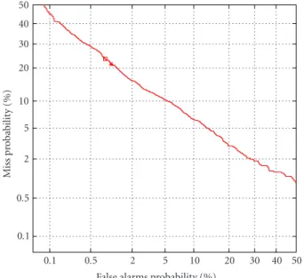
is monotonous and decreasing. Furthermore, it has become a standard to plot the error curve on a normal deviate scale [47] in which case the curve is known as the detection er-ror trade-offs (DETs) curve. With the normal deviate scale, a speaker recognition system whose true speaker and impos-tor scores are Gaussians with the same variance will result in a linear curve with a slope equal to −1. The better the system is, the closer to the origin the curve will be. In prac-tice, the score distributions are not exactly Gaussians but are quite close to it. The DET curve representation is therefore more easily readable and allows for a comparison of the sys-tem’s performances on a large range of operating conditions. Figure 6shows a typical example of a DET curves.
Plotting the error rates as a function of the threshold is a good way to compare the potential of different methods in laboratory applications. However, this is not suited for the evaluation of operating systems for which the threshold has been set to operate at a given point. In such a case, systems are evaluated according to a cost function which takes into
False alarms probability (%)
0.1 0.5 2 5 10 20 30 40 50 Mi ss pr ob ab ili ty (% ) 0.1 0.5 2 5 10 20 30 40 50
Figure 6: Example of a DET curve.
account the two error rates weighted by their respective costs, that is C =CfaPfa+ CfrPfr. In this equation, Cfaand Cfr are
the costs given to false acceptances and false rejections, re-spectively. The cost function is minimal if the threshold is correctly set to the desired operating point. Moreover, it is possible to directly compare the costs of two operating sys-tems. If normalized by the sum of the error costs, the cost C can be interpreted as the mean of the error rates, weighted by the cost of each error.
Other measures are sometimes used to summarize the performance of a system in a single figure. A popular one is the equal error rate (EER) which corresponds to the operat-ing point where Pfa=Pfr. Graphically, it corresponds to the
intersection of the DET curve with the first bisector curve. The EER performance measure rarely corresponds to a re-alistic operating point. However, it is a quite popular mea-sure of the ability of a system to separate impostors from true speakers. Another popular measure is the half total error rate (HTER) which is the average of the two error rates Pfaand Pfr.
It can also be seen as the normalized cost function assuming equal costs for both errors.
Finally, we make the distinction between a cost obtained with a system whose operating point has been set up on de-velopment data and a cost obtained with a posterior mini-mization of the cost function. The latter is always to the ad-vantage of the system but does not correspond to a realistic evaluation since it makes use of the test data. However, the difference between those two costs can be used to evaluate the quality of the decision making module (in particular, it evaluates how well the decision threshold has been set).
5.3. Factors affecting the performance and evaluation paradigm design
There are several factors affecting the performance of a speaker verification system. First, several factors have an
impact on the quality of the speech material recorded. Among others, these factors are the environmental condi-tions at the time of the recording (background noise or not), the type of microphone used, and the transmission channel bandwidth and compression if any (high bandwidth speech, landline and cell phone speech, etc.). Second are factors con-cerning the speakers themselves and the amount of train-ing data available. These factors are the number of traintrain-ing sessions and the time interval between those sessions (sev-eral training sessions over a long period of time help cop-ing with the long-term variability of speech), the physical and emotional state of the speaker (under stress or ill), the speaker cooperativeness (does the speaker want to be rec-ognized or does the impostor really want to cheat, is the speaker familiar with the system, and so forth). Finally, the system performance measure highly depends on the test set complexity: cross gender trials or not, test utterance dura-tion, linguistic coverage of those utterances, and so forth. Ideally, all those factors should be taken into account when designing evaluation paradigms or when comparing the per-formance of two systems on different databases. The ex-cellent performance obtained in artificial good conditions (quiet environment, high-quality microphone, consecutive recordings of the training and test material, and speaker will-ing to be identified) rapidly degrades in real-life applica-tions.
Another factor affecting the performance worth noting is the test speakers themselves. Indeed, it has been observed several times that the distribution of errors varies greatly be-tween speakers [48]. A small number of speakers (goats) are responsible for most of the nondetection errors, while an-other small group of speakers (lambs) are responsible for the false acceptance errors. The performance computed by leav-ing out these two small groups are clearly much better. Evalu-ating the performance of a system after removing a small per-centage of the speakers whose individual error rates are the higher may be interesting in commercial applications where it is better to have a few unhappy customers (for which an alternate solution to speaker verification can be envisaged) than many ones.
5.4. Typical performance
It is quite impossible to give a complete overview of the speaker verification systems because of the great diversity of applications and experimental conditions. However, we con-clude this section by giving the performance of some systems trained and tested with an amount of data reasonable in the context of an application (one or two training sessions and test utterances between 10 and 30 seconds).
For good recording conditions and for text-dependent applications, the EER can be as low 0.5% (YOHO database), while text-dependent applications usually have EERs above 2%. In the case of telephone speech, the degradation of the speech quality directly impacts the error rates which then range from 2% EER for speaker verification on 10 digit strings (SESP database) to about 10% on conversational speech (Switchboard).
6. EXTENSIONS OF SPEAKER VERIFICATION
Speaker verification supposes that training and test are com-posed of monospeaker records. However, it is necessary for some applications to detect the presence of a given speaker within multispeaker audio streams. In this case, it may also be relevant to determine who is speaking when. To handle this kind of tasks, several extensions of speaker verification to multispeaker case have been defined. The three most com-mon ones are briefly described below.
(i) The n-speaker detection is similar to speaker verifica-tion [49]. It consists in determining whether a target speaker speaks in a conversation involving two speak-ers or more. The difference from speaker verification is that the test recording contains the whole conversation with utterances from various speakers [50,51]. (ii) Speaker tracking [49] consists in determining if and
when a target speaker speaks in a multispeaker record. The additional work as compared to the n-speaker detection is to specify the target speaker speech seg-ments (begin and end times of each speaker utterance) [51,52].
(iii) Segmentation is close to speaker tracking except that no information is provided on speakers. Neither speaker training data nor speaker ID is available. The number of speakers is also unknown. Only test data is available. The aim of the segmentation task is to de-termine the number of speakers and when they speak [53,54,55,56,57,58,59]. This problem corresponds to a blind classification of the data. The result of the segmentation is a partition in which every class is com-posed of segments of one speaker.
In the n-speaker detection and speaker tracking tasks as described above, the multispeaker aspect concerned only the test records. Training records were supposed to be monos-peaker. An extension of those tasks consists in having mul-tispeaker records for training too, with the target speaker speaking in all these records. The training phase then gets more complex, requiring speaker segmentation of the train-ing records to extract information relevant to the target speaker.
Most of those tasks, including speaker verification, were proposed in the NIST SRE campaigns to evaluate and com-pare performance of speaker recognition methods for mono-and multispeaker records (test mono-and/or training). While the set of proposed tasks was initially limited to speaker verification task in monospeaker records, it has been enlarged over the years to cover common problems found in real-world appli-cations.
7. APPLICATIONS OF SPEAKER VERIFICATION
There are many applications to speaker verification. The applications cover almost all the areas where it is desir-able to secure actions, transactions, or any type of interac-tions by identifying or authenticating the person making the transaction. Currently, most applications are in the banking