ASSESSMENT OF THE LAKE WINNIPEG WATER QUALITY MONITORING NETWORK
ASSESSMENT OF THE LAKE WINNIPEG WATER QUALITY MONITORING NETWORK RESEARCH REPORT # R-1197 Par Bahaa Khalil Dan Beveridge André St-Hilaire Taha B.M.J. Ouarda
Institut national de la recherche scientifique Centre Eau, Terre et Environnement
(INRS-ETE)
490 De la Couronne, Québec, G1K 9A9
March 2010
Suggested citation:
Khalil, B., D. Beveridge, A. St-Hilaire, T.B.M.J. Ouarda. 2010. Assessment of the Lake Winnipeg water quality monitoring network. Research report R-1197, INRS-ETE. vi+182 pages.
© INRS-ETE, 2010
LIST OF TABLES ... iv LIST OF FIGURES ... vi 1 INTRODUCTION ... 1 2 DATA ... 3 3 METHODOLOGY ... 5 3.1 Preliminary analyses ... 5
3.2 Isotope station number and configuration ... 6
3.2.1 Kriging ... 6
3.2.2 Cross-validation ... 7
3.2.3 Improving prediction with additional predictors ... 8
3.3 Water quality variables ... 10
3.3.1 Background on record augmentation and extension approaches... 11
3.3.2 Proposed approach ... 18
3.4 Sampling frequency ... 24
3.4.1 Semi-variogram approach ... 25
3.4.2 Confidence Interval width ... 26
4 RESULTS ... 30
4.1 Preliminary analyses ... 30
4.2 Isotope station number and configuration ... 41
4.3 Water quality variables ... 50
4.3.1 Rationalisation results ... 50
4.3.2 Information transfer ... 54
4.4 Sampling frequency ... 58
4.4.1 Semi-variogram approach ... 58
4.4.2 Confidence Interval approach ... 62
5 CONCLUSIONS ... 68 5.1 Discussion ... 68 5.2 Future analysis ... 69 5.3 Recommendations ... 69 6 REFERENCES ... 71 Appendix 1. Kriging ... 74
Appendix 2. Principal Component Analysis ... 75
Appendix 3. Non-Metric Multidimensional Scaling ... 76
Appendix 4. Data Preliminary analyses ... 77
Appendix 5. Detailed results for the assessment of water quality variables ... 130
Appendix 6: Detailed results for the assessment of Sampling Frequency Confidence Interval approach ... 148
Table 1. Water quality variables ... 4
Table 2. Location MB05SBS126, descriptive statistics ... 31
Table 3. Location MB05SBS126, Kolmogrov-Smirnov test ... 31
Table 4. Mann-Kendall nonparametric trend test results ... 39
Table 5. Kolmogrov-Smirnov test results summary ... 40
Table 6. Measures of δ18O and δ2H kriging model performance ... 43
Table 7. Stations highlighted by kriging analysis for potential removal or retention. ... 49
Table 8. Variable to discontinue and its best auxiliary variable ... 52
Table 9. Combinations of variables to discontinue ... 53
Table 10. Average error measures for record-extension techniques ... 58
Table 11. Error percentage expected based on collecting 6 samples per year ... 65
Table 12. Error percentage expected based on collecting 12 samples per year ... 65
Table 13. Error percentage expected based on collecting 26 samples per year ... 66
Table 14. Error percentage expected based on collecting 52 samples per year ... 66
Table 15 Location MB05RAS078, WQ variables descriptive statistics ... 77
Table 16 Location MB05RAS078, WQ variablesKolmogrov-Smirnov test ... 77
Table 17 Location MB05RBS003, WQ variables descriptive statistics ... 84
Table 18 Location MB05RBS003, WQ variables Kolmogrov-Smirnov test ... 84
Table 19 Location MB05SAS004, WQ variables descriptive statistics ... 91
Table 20 Location MB05SAS004, WQ variables Kolmogrov-Smirnov test ... 91
Table 21 Location MB05SAS004, transformed WQ variables descriptive statistics ... 92
Table 22 Location MB05SAS004, transformed WQ variables Kolmogrov-Smirnov test 92 Table 23. Location MB05SBS126, WQ variables descriptive statistics ... 99
Table 24. Location MB05SBS126, WQ variablesKolmogrov-Smirnov test ... 99
Table 25. Location MB05SCS005, WQ variables descriptive statistics ... 106
Table 26. Location MB05SCS005, WQ variablesKolmogrov-Smirnov test ... 106
Table 27. Location MB05SHS004, WQ variables descriptive statistics ... 113
Table 28. Location MB05SHS004, WQ variablesKolmogrov-Smirnov test ... 113
Table 29. Location MB05SHS004, transformed WQ variables descriptive statistics .... 114
Table 30. Location MB05SHS004, transformed WQ variables Kolmogrov-Smirnov test ... 114
Table 31. Location MB05SHS014, WQ variables descriptive statistics ... 121
Table 32. Location MB05SHS014, WQ variables Kolmogrov-Smirnov test ... 121
Table 33. Location MB05SHS014, transformed WQ variables descriptive statistics .... 122
Table 34. Location MB05SHS014, transformed WQ variables Kolmogrov-Smirnov test ... 122
Table 38. Variable to discontinue and its best auxiliary variable (MB05SAS004) ... 134
Table 39. Variable to discontinue and its best auxiliary variable (MB05SBS126) ... 134
Table 40. Variable to discontinue and its best auxiliary variable (MB05SCS005) ... 135
Table 41. Variable to discontinue and its best auxiliary variable (MB05SHS004) ... 135
Table 42. Variable to discontinue and its best auxiliary variable (MB05SHS014) ... 135
Table 43. Combinations of two variables to discontinue ... 136
Table 44. Combinations of three variables to discontinue ... 138
Table 45. Combinations of four variables to discontinue ... 142
Figure 1. Flow chart of the proposed rationalization approach (Khalil et al., 2010a) ... 22
Figure 2. Semi-variogram parameters ... 26
Figure 3. Location MB05SBS126, WQ variables Box-plots ... 33
Figure 4. Location MB05SBS126, WQ variables Corellogram ... 36
Figure 5. Isotope stations plotted along the first two principal components of a PCA on the predictor variables. ... 41
Figure 6. Isotope stations plotted in two-dimensional NMDS space. ... 42
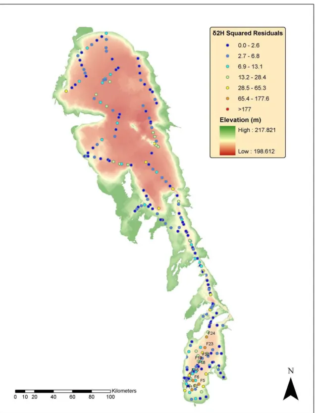
Figure 7. Squared residual from leave-one-out cross-validation of δ2H. ... 45
Figure 8. δ2H kriging variance from leave-one-out cross-validation. ... 46
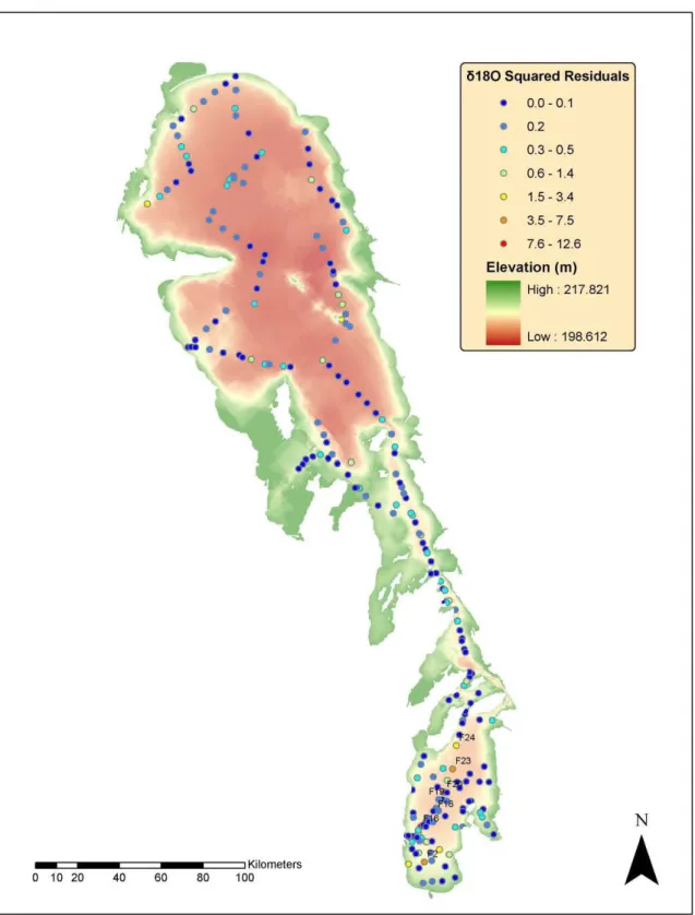
Figure 9. Squared residual from leave-one-out cross-validation of δ18O. ... 47
Figure 10. δ18O kriging variance from leave-one-out cross-validation. ... 48
Figure 11. Cluster tree for water quality variables at MB05SBS126 ... 51
Figure 12. Box plots of the ratio U for the mean and standard deviation ... 55
Figure 13. Box plots of the ratio U for different percentiles ... 56
Figure 14. BIASr of the tested extension techniques in estimating various percentiles ... 56
Figure 15. RMSEr of the tested extension techniques in estimating various percentiles ... 57
Figure 16. Variogram for CaCO3 measured at MB05RAS078 (lag class interval =1) ... 60
Figure 17. Variogram for CaCO3 measured at MB05RAS078 (lag class interval =4) ... 61
Figure 18. Number of samples vs expected error for CaCO3 measured at MB05SBS126 ... 63
Figure 19. Location MB05RAS078, WQ variables Box-plots ... 78
Figure 20. Location MB05RAS078, WQ variables Corellogram ... 81
Figure 21. Location MB05RBS003, WQ variables Box-plots ... 85
Figure 22. Location MB05RBS003, WQ variables Corellogram... 88
Figure 23. Location MB05SAS004, WQ variables Box-plots ... 93
Figure 24. Location MB05SAS004, WQ variables Corellogram ... 96
Figure 25. Location MB05SBS126, WQ variables Box-plots ... 100
Figure 26. Location MB05SBS126, WQ variables Corellogram ... 103
Figure 27. Location MB05SCS005, WQ variables Box-plots ... 107
Figure 28. Location MB05SCS005, WQ variables Corellogram ... 110
Figure 29. Location MB05SHS004, WQ variables Box-plots ... 115
Figure 30. Location MB05SHS004, WQ variables Corellogram ... 118
Figure 31. Location MB05SHS014, WQ variables Box-plots ... 123
Figure 32. Location MB05SHS014, WQ variables Corellogram ... 126
Figure 33. Cluster tree for water quality variables at MB05RAS078 ... 130
Figure 34. Cluster tree for water quality variables at MB05RBS003 ... 130
Figure 35. Cluster tree for water quality variables at MB05SAS004 ... 131
Figure 36. Cluster tree for water quality variables at MB05SBS126 ... 131
Figure 37. Cluster tree for water quality variables at MB05SCS005 ... 132
Figure 38. Cluster tree for water quality variables at MB05SHS004 ... 132
1 INTRODUCTION
Water quality monitoring programs aid in the understanding of various water quality processes and provide water managers with the necessary information for water resources management, in general, and water quality management, in particular (Khalil et al., 2010a).
Water quality monitoring programs encompass a variety of activities that include the following: definition of the monitoring purpose and desired information, monitoring network design, sampling protocol design, laboratory analysis, data verification and storage, and data analysis (Khalil and Ouarda, 2009).
The design of monitoring networks is the translation of the monitoring objectives to specify the sampling sites, sampling frequency and variables to be measured (Khalil et al., 2010a). The quality of a water body is usually described by a set of physical, chemical and biological variables that are mutually interrelated. Water quality can be defined in terms of one variable or hundreds of compounds and for multiple usages. This is a very complex issue because there are numerous variables that can represent surface water quality (Sanders et al., 1983; Harmancioglu et al., 1999).
Selection of the initial water quality variables to measure, or the addition of new variables, is primarily based on the monitoring objectives, facilities and available budget. However, statistical approaches are used if the objective is to reduce the number of water quality variables measured.
Another important aspect of water quality monitoring network design is the sampling frequency. Sampling frequency affects not only data utility but also operational cost. With too-frequent sampling, the obtained information is redundant and costly, while infrequent sampling may limit the precision. Statistical methods proposed for the
assessment and calculation of sampling frequencies are directly related to the monitoring objectives and the data analysis methods. For instance, the effective sampling method proposed by Lettenmaier (1976) is used to assess the sampling frequency when the monitoring objective is to detect temporal trends.
In large continuous water bodies such as lakes, sampling location and spatial density of sampling sites must be selected such that the spatial variability of water quality is captured without spending resources in acquiring redundant information.
The readers are referred to Khalil and Ouarda (2009) for more detailed information regarding the statistical approaches used to assess and redesign water quality monitoring networks.
The main goal of this study was to provide a first statistical assessment of the the current applied monitoring activities in Lake Winnipeg, Manitoba, Canada. As such, this firs report does not provide an assessment of the complete water quality data base gathered on Lake Winnipeg. The specific objectives of this report are the assessment of:
the number of isotope stations and their spatial configuration; the number of water quality variables to measure; and
2 DATA
Two water quality datasets were used in this study. The first comprised the δ18O and δ2H
isotope data collected between 14/09/2009 and 04/10/2009. The samples were collected once at each of 240 locations throughout the lake. As such, the isotope database is perhaps de most dense sampling network on Lake Winnipeg.
The second dataset used in this study were provided by the Water Quality Management Section, Manitoba Water Stewardship, Winnipeg. The database consisted of 168 sampling sites, at which 13 water quality variables were measured on an irregular basis (Table 1). Of 168 sampling locations, 55 were sampled only once between 1992 and 2008. Only seven sampling sites were sampled more than 30 times during this period. These seven sampling sites were selected in this study for assessment of the number of water quality variables to measure and the sampling frequencies of these variables. The selected sampling site codes are as follows: MB05RAS078; MB05RBS003; MB05SAS004; MB05SBS126; MB05SCS005; MB05SHS004; and MB05SHS014. The seven selected sites represent the three main regions of Lake Winnipeg. The sampling sites MB05RAS078 and MB05RBS003 are located in the narrows. Sites MB05SAS004, MB05SBS126 and MB05SCS005 represent the south basin, and sites MB05SHS004 and MB05SHS014 represent the north basin.
Table 1. Water quality variables
Water Quality Variable Symbol units
Alkalinity Total CaCO3 CaCO3 mg/L
Alkalinity Total HCO3 HCO3 mg/L
Chloride Dissolved Cl mg/L
Colour Colour CU
Conductivity (at 25Cο) EC US/cm
Hardness Total CaCO3 H. CaCO3 mg/L
pH pH pH units
Sodium Total Na mg/L
Sulphate Dissolved SO4 mg/L
Water Temperature (Field) Temp. Deg C
Total Dissolved Solids (at 180 Cο) TDS mg/L at180C
Total Suspended Solids TSS mg/L
3 METHODOLOGY
The methodology consists of several steps. The first step included preliminary analyses, followed by statistical approaches to assess the number of sampling sites, water quality variables and sampling frequency. The objectives of the preliminary analyses were to understand the characteristics of the available water quality data and verify the statistical assumptions required to apply the designed statistical approaches to the assessment and redesign of the monitoring network. The following subsections present the preliminary analyses, sampling sites assessment, water quality variables assessment and the sampling frequency assessment.
3.1 Preliminary analyses
The preliminary analyses included descriptive statistics as well as tests to check normality, autocorrelation and existence of trend. The descriptive statistics included measures of central tendency, variability, skewness and kurtosis. The mean and median were computed to characterise the central tendency. The minimum, maximum, range, standard deviation and variance were computed to characterise the variability. The skewness is a measure of symmetry, or more precisely, the lack of symmetry. A distribution, or data set, is symmetric if it looks the same to the left and right of the centre point. The kurtosis is a measure of whether the data are peaked or flat relative to a normal distribution; i.e., data sets with high kurtosis tend to have a distinct peak near the mean, decline rather rapidly, and have heavy tails. Data sets with low kurtosis tend to have a flat top near the mean rather than a sharp peak.
The box-and-whisker plot (boxplot) is a common five-number summary of the distribution of a variable in graphical form. The box extends from the 25th to the 75th percentile and is crossed by a bar at the median. The H-spread is a term given to the differences between the 25th and the 75th percentile. A step is 1.5 times the H-spread, and
the whiskers extend one step. Values that are more extreme, but within two steps, are considered outliers and indicated with an “o”. Values outside are considered extreme outliers and indicated with an asterisk “*”. Boxplots may also be used for spatial or temporal comparison. Comparing the boxplots of the same variable at different locations, or at different consequent years, provides a visual inspection for possible trends, outliers, and data distribution.
The Mann-Kendall nonparametric trend test was employed to test for the existence of a trend. Mann (1945) first suggested using the significance test for Kendall's tau, where the x variable is time, as a test for trend (monotonic change). No assumption of normality is required, but there must be no serial correlation for the resulting p-values to be correct.
The autocorrelation functions (ACFs) for the available water quality variables were also computed. The plot of the autocorrelation function (ACF) against the lag time is called a correlogram. It should be mentioned that trends affect the correlogram function. Therefore, the time series were adjusted (de-trended) before creating the correlogram. To check whether the water quality data followed a normal distribution, the Kolmogorov-Smirnov test for normality was performed.
3.2 Isotope station number and configuration 3.2.1 Kriging
We used kriging to identify water quality stations that contribute the most and least information to prediction maps. Kriging is an interpolation method that predicts the value of a variable at an unmeasured location as a function of observed data from nearby locations. The spatial dependence between points is expressed using a variogram. The variogram captures how the differences in values of points change as the points become further away from each other. Kriging produces an optimal prediction, in the sense that errors and bias are minimized (Journel and Huijbregts 1978).
Before kriging, we will explore the data using techniques such as normal QQ plots, trend analysis, and semivariogram clouds to determine whether the water quality data require transformation or trend removal.
Once the data are prepared for kriging, the variogram model is fit, i.e. we will determine the optimum values of a few variogram parameters. The sill is the value at which the variance no longer increases and should be close to the sample variance. The range is the distance at which the semivariogram model reaches the sill; beyond this distance, observations appear independent. Anisotropy is the presence of directional dependence, i.e. there is a difference in the correlation between points along different axes. If the data are anisotropic, the direction of strongest correlation defines the direction of the major range. The minor range is perpendicular to the major range and its length relative to the major range is expressed as the anisotropy ratio. Different mathematical functions can be used to model the semivariance, e.g. linear, spherical, gaussian or exponential. The best type of function will be iteratively determined and based on that which yields the smallest nugget effect and Root Mean Square Error (RMSE). The nugget effect represents measurement error or variation at a spatial scale finer than the data.
Once the variogram model is fit, the water quality data will be predicted using ordinary kriging. We will use ordinary kriging which assumes that the mean is constant within the neighborhoud of the point to be estimated, but allows this mean to vary as an unknown constant trend in the whole region.
Kriging is briefly summarized in Appendix 1. It is well-described by Journel and Huijbregts (1978).
3.2.2 Cross-validation
In cross-validation, data are divided into a calibration set, which is used for parameter estimation, and a validation set, with which the results of the calibration set are validated. It is typically used to assess how the results of an analysis based on one dataset will generalize to a different data set. We used it to identify water quality stations that are particularly useful or not useful in predicting water quality.
We used the leave-one-out cross-validation procedure in which one station at a time will be left out as validation data while a kriging map is created from the remaining, i.e. n-1
data, where n=the number of water quality stations, e.g. n=237 in the case of the isotope data. This process will be repeated n times.
Each time the training process is repeated, the residual and the kriging variance will be calculated. The residual is the difference between the value that the kriging model predicts at the location of the removed station and the observed value. A large residual likely indicates that the missing station is important to prediction. Conversely, a small residual likely indicates that there is significant redundancy between the missing station and its neighbours and that that location can be predicted with less cost. The kriging variance, also known as the kriging error, is by definition minimized in a kriging model, so when a removing a station produced a kriging map with high variance, that station is likely important to prediction. Conversely, when removing a station yields a kriging map with relatively low variance, it is likely redundant with its neighbours.
3.2.3 Improving prediction with additional predictors
The kriging method used above only used the relative position and orientation of water quality stations to predict the values of water quality parameters. Other factors influence water quality and are potentially measured directly or indirectly from available data. Two such factors are water depth, i.e. the elevation of the lake bed, and the proximity of a water quality station to the mouth of a contributing river.
Lake bathymetry data are available. Lake bed elevation will be kriged to predict the elevation at water quality stations.
Lake and river hydrography is available. The distance of a water quality station to the mouth of major contributing rivers will be calculated.
These additional variables can potentially improve the quality of prediction. Unfortunately, kriging can only use two predictive variables at a time. Co-kriging allows information of an auxiliary variable (the co-variable) to be used in the prediction of the variable of interest. The co-variable does not need to be measured at the same locations
as the target variable but it does need to demonstrate a spatial structure and correlation and covariance over space with the target variable.
To incorporate more than three predictive variables at a time, we have to use Principal Component Analysis (PCA). PCA can compress the information contained in many variables into the small number of axes permitted in kriging. PCA transforms a large number of intra-correlated variables into uncorrelated variables called principal components. In the process, much of the variability in the original dataset is explained in a few e.g. two or three, principal components. PCA is briefly described in Appendix 2. We conducted PCA on a dataset containing geographic coordinates, elevation, and distances to the mouths of contributing rivers of water quality stations. The first principal components was used to define a new coordinate system onto which the water quality stations were be projected. Once the stations are located in this new space, we can use the leave-one-out cross-validation procedure outlined above to identify water quality stations that are more or less important when kriging prediction maps.
A variety of measures were be used to evaluate the performance of the kriging model. The Mean Error is the mean difference between observed and predicted values and is ideally 0. The Median Square Prediction Error (MSPE) is calculated by squaring all the errors and taking their median; it is ideally a small number. The Mean Square Normalized Error (MSNE) was calculated as in Equation 1.
n rror standard e residual MSNE 2 (1)
where n is the number of water quality stations. MSNE is ideally close to 1. The correlation between observed and predicted values, ideally 1, and the correlation between predicted and residual, ideally 0, will also be used.
3.3 Water quality variables
A review of the literature reveals that the most commonly used statistical approach to reduce the number of variables being measured is the correlation-regression (CR) approach. The CR approach is based on three steps. First, correlation analysis is used to assess the level of association among the variables being measured. If high correlation exists among the variables, some of the information produced may be redundant. Second, the water quality variables to be continuously measured or discontinued are selected. This step is based on some subjective criteria, such as the significance of the variable, the presence of the variable in local or international standards, and the cost of laboratory analysis. Third, the reconstitution of information about the discontinued variables using auxiliary variables from the continuously measured variables is examined.
The main advantage of the CR approach is that it allows the reconstitution of information about the discontinued variables using regression analysis. However, Khalil et al. (2010a) identified three main deficiencies in the CR approach as commonly practiced for water quality variable reduction. The first deficiency involves the method used to identify highly associated variables. The correlation coefficient is commonly used as a criterion to assess the level of association, but selection of the proper threshold above which a correlation coefficient can be considered sufficient to associate two variables can be problematic. Assessment of the correlation coefficient is always based on subjective preference. Thus, studies using the same variables but performed by different investigators may lead to different results. The second deficiency is the absence of a criterion to identify the combination of variables that should be continuously measured or discontinued. The third deficiency is that the use of regression analysis to reconstitute information about discontinued variables often results in an underestimation of the variance in the extended records (Alley and Burns, 1983; Hirsch, 1982).
Khalil et al. (2010a) modified the CR approach to overcome these three deficiencies by using criteria from record-augmentation procedures to identify a correlation coefficient threshold. To identify optimal combinations of variables to be continuously measured and variables to discontinue, Khalil et al. (2010a) proposed an information performance index to
evaluate different combinations of variables. For reconstitution of information about the discontinued variables, Khalil et al. (2010a) recommended the use of the maintenance of variance extension technique type 3 (MOVE3), whereas the regression technique was recommended for the reconstitution of missing values.
In this study, the approach proposed by Khalil et al. (2010a) was applied to identify optimal combinations of variables to be continuously measured and variables to discontinue. The following subsection provides background on the record augmentation and extension approaches. The second subsection presents the proposed approach.
3.3.1 Background on record augmentation and extension approaches
Estimation of the mean and variance of streamflows or other hydrological variables at a short-record gauge from a longer, continuously measured gauge is termed record augmentation (Vogel and Stedinger, 1985). However, the extension of monthly, weekly or daily records is termed record extension. The following subsections present a short review of record augmentation and record extension approaches.
3.3.1.1 Record augmentation
Assume that the measured variable y has n1 years of data and the measured variable
xhas n1n2 years of data, from which n1 are concomitant with the data observed for y, illustrated as follows: 1 2 1 1 1 1 ,..., , , ,..., , , ,..., , , 3 2 1 2 1 3 2 1 n n n n n n y y y y x x x x x x x
In the case of water quality variables reduction, year n1 can be considered as the year where assessment and selection took place. After n1 years, assessment of the water
quality variables reveals that measurement of the variable y can be stopped, whereas measurement of variablex can be continued. Assume that after n2 years our interest is to
estimate the mean y and the variance 2y of the variable y as accurately as possible. Matalas and Jacobs (1964) developed a procedure for obtaining unbiased estimators of both y and y2, showing that the mean value (ˆy) of the extended series can be determined by the following:
) ( ˆ ˆ 2 1 2 1 2 1 n n x x n y y (2)
where y1 and x1 are the mean values of y and i x based on short records i i1,...,n1; x2 is
the mean value of x observed during the period i in1 1,....,n2; and the parameter ˆ is
the estimated regression coefficient. Based on this formulation, it is possible to show (Cochran, 1953) that the variance of ˆy is given by the following:
3 1 1 ˆ 1 2 2 2 1 2 1 2 n n n n n Var y y (3) where 2 y is the population variance of y, and
is the population correlation between x and y. For practical use, these values may be replaced by their estimates based on the1
n years of data (Ouarda, et al., 1996). To assess whether the extended series provides additional information on the variable y, the variance above must be compared with the variance obtained from the short record (2y n1), and the condition for an improved
estimator (smaller variance) of the mean is given by the following:
) 2 ( 1 1 2 n
(4)Therefore, estimation of the mean from the extended series is profitable only if the correlation coefficient between the two variables exceeds
121 2
n (Ouarda et al., 1996). If the variance of the y-series is of interest, one can proceed as in the case of the mean. Matalas and Jacobs (1964) obtained the following expression for the unbiased variance estimator ˆ2 y : ) ˆ ( 2 1 ) 1 )( 3 ( 3 1 ˆ ˆ 2 1 2 1 1 1 2 1 1 2 1 2 2 2 x y x y n s s n n n n n n s (5) where 2 x
s is the variance estimate based on the entire x-series, and sy1,sx1 are the standard deviations of y and x based on the short records i1,...,n1. Moreover, Matalas and Jacobs (1964) showed that the variance of the variance estimator (
ˆ2y Var ) is given by the following:
( ) ) 3 ( ) 1 ( 1 2 ˆ 2 1 2 2 1 4 2 1 4 2 A B C n n n n n Var y y y (6) where
4 3 4 2 2 3 4 4 5 8 6 2 1 1 2 1 1 1 2 1 1 1 1 1 2 n n n n n n n n n n n n n A (7)
2 3 4 2 3 2 3 5 2 4 14 2 5 6 2 6 1 1 1 2 1 1 1 1 2 1 1 2 1 1 1 2 n n n n n n n n n n n n n n n B (8)
2 3 4 1 2 3 2 4 1 3 2 2 1 5 2 3 1 2 1 1 1 2 1 1 1 2 1 1 1 2 1 1 1 2 1 n n n n n n n n n n n n n n n n n C (9)The first term on the right-hand side in Equation 6 is equal to the variance of the variance estimator based on the n1 years of the y-series; therefore, estimation is profitable when:
A AC B B 4 )/2 ( 2 2 (10)
Khalil et al. (2010a) used Equations 4 and 10 as criteria for assessment of the required correlation coefficient threshold and identification of highly associated pairs of variables. By using such criteria, Khalil et al. (2010a) overcame the first disadvantage of the CR approach. In this study, the higher correlation coefficient obtained from Equations 4 and 10 is used as a criterion to evaluate the correlation coefficients among water quality variables measured at the seven selected locations.
3.3.1.2 Record extension
To estimate records of the discontinued variable y for the period n11 through n2 years,
the simple linear regression of y on x can be used.
i
i a bx
yˆ (11)
where yˆi are the estimated values of y for in11 n,... 2, and a and b are the constant
and slope of the regression equation, respectively. The parameters a and b are the values that minimise the sum of the squared differences between the estimated and measured y
values. The solutions of a and b are found by solving the normal equations (Draper and Smith, 1966, p. 59). The optimal solution to equation 11 is the following:
) ( ) ( ˆ y1 r s 1 s 1 x x1 yi y x i (12)
The use of regression analysis often results in underestimation of the variance in the extended records (Alley and Burns, 1983). Matalas and Jacobs (1964) demonstrated that unbiased estimates of the mean (ˆy) and variance ( ˆ2
y
) are obtained if the following equation is used:
y i i x y i y r s s x x r s e y 2 12 1 1 1 1 1 ( )( ) 1 ˆ (13)where is a constant that depends on n1 and n2 (see Hirsch, 1982); r is the
product-moment correlation coefficient between the n1 concurrent measurements of x and y; and
i
e is a normal independent random variable with zero mean and unit variance. However, due to the presence of an independent noise component (ei), the problem in using Equation 13 is that studies of the same sequence of x and y by different investigators will almost certainly lead to different values of yˆi (Hirsch, 1982; Alley and Burns, 1983).
Hirsch (1982) suggested two other methods, referred to as MOVE1 and MOVE2 (Maintenance of Variance, Types 1 and 2). In MOVE1, Hirsch (1982) chose the estimators of a and b so that if Equation 10 is used to generate an entire sequence yˆi for
2 1 ,...,
1 n n
i , the short sample moments y1 and s2y1 would be reproduced. Similarly, in
MOVE2, Hirsch (1982) chose a and b so that if Equation 11 is used to generate an entire sequence yˆi for i1,...,n1n2, the unbiased estimates ˆy and ˆ2y would be estimated.
Hirsch (1982) evaluated the MOVE1, MOVE2, regression and regression-plus-noise methods using a Monte Carlo study and an empirical analysis. Both the Monte Carlo study and the empirical analysis showed that regression cannot be expected to provide records with the appropriate variability.
In practice, Equation 11 is used to generate the yˆi only for in11,...,n1n2. This suggests that Hirsch (1982) used estimators of a and b that did not achieve what he intended (Vogel and Stedinger, 1985). MOVE3 was then proposed by Vogel and Stedinger (1985). In MOVE3, the main goal is to select a and b in Equation 11 so that the resultant sequence of n1n2 values
y1,...,yn1,yˆn11,...,yˆn1n2
has a mean ˆy and variance ˆ2y
(the Matalas and Jacobs estimators; Equations 2 and 5). Estimates of a and b for the MOVE3 method are obtained by rewriting Equation 11 as follows:
2
ˆ a b x x
yi i (14)
where estimates of a and b are obtained as follows:
n1 n2 ˆ n1y1
n2 a y (15)
2
1 2 2 2 2 2 1 1 2 1 1 2 2 1 2 1 ˆ 1 ˆ ˆ 1 x y y y y n s n y n a n s n n b (26)The Kendall-Theil robust line (KTRL) method has been proposed as an analogue to regression, with the advantage of being robust in the presence of extreme values. The KTRL method is based on Kendall’s rank correlation coefficient (tau), which is used to
test for any monotonic, and not necessarily linear, dependence of y on x. Related to tau is a robust nonparametric line that is applicable when y is linearly related to x. This line will not depend on the normality of residuals for the validity of significance tests, nor will it be strongly affected by extreme values, in contrast to regression (Helsel and Hirsch, 2002).
A robust estimate of the slope for this nonparametric fitted line was first described by Theil (1950). The Theil slope is estimated by comparing each data pair to all others in a pair-wise fashion. An n-element data set of (x, y) pairs will result in n (n-1)/2 pair-wise comparisons. For each of these comparisons, a slope /y x is computed. The median of all possible pair-wise slopes is taken as the nonparametric slope estimate (bK):
n j n i j i x x y y median b i j i j K ..., 3 , 2 1 ,... 2 , 1 (37)
The intercept (aK) is defined as follows:
) ( * ) (y b median x median aK K (48)
This formula assures that the fitted line goes through the point [median (x), median (y)]. This is analogous to regression, where the fitted line always goes through the point [mean (x), mean (y)]. The parameter bK is an unbiased estimator of the slope of a linear relationship, and b from regression is also an unbiased estimator. However, the variances of the estimators differ. When the residuals from the true linear relationship are normally distributed, regression is slightly more efficient (has a lower variance) than the KTRL method. When residuals depart from normality (i.e., are skewed or prone to extreme values), then bK can be much more efficient than the regression slope (Hirsch et al., 1991; Helsel and Hirsch, 2002).
Khalil et al. (2010b) generated a modified KTRL method, referred to as KTRL2, that utilises MOVE techniques to reduce the bias in the estimation of the variance while incorporating the robustness of the KTRL method in the presence of extreme values. The KTRL2 method proposed by Khalil et al. (2010b) follows the KTRL method, but with a modification of the intercept (aq) and slope (bq). Its objective is to produce records with sample cumulative distribution functions (CDFs) that are close approximations of the CDFs of the actual records. The developmental goal of KTRL2 is to find the values of aq and bq
in Equation 11 that minimise the error when estimating the y percentiles; aq and bq are defined as follows: th th th th th th i j i j q j i j i x q x q y q y q median b 95 ..., 15 , 10 90 ,... 10 , 5 ) ( ) ( ) ( ) ( (59)
The intercept is defined as follows:
) ( * ) (y b median x median aq q (206)
where q(y) and q(x) are the percentiles of y and x estimated during the period of concurrent records. Percentiles are obtained for the range of the 5th, 10th… 95th percentile. Thus, a set of 19 (x, y) pairs of percentiles will result in 171 [n (n-1)/2 = 19 (19-1)/2] pair-wise comparisons. For each of these comparisons, a slope /y x is computed, and the median of the 171 possible pair-wise slopes is taken as the slope estimate. Consequently, the objective in developing the KTRL2 method was to minimise the error in estimating the y percentiles rather than to minimise the error in estimating the y records.
3.3.2 Proposed approach
The approach proposed by Khalil et al. (2010a) consists of four main steps. The first step is to assess the level of association among the variables being measured and to define the groups of variables that are highly associated. Then, for each highly associated group of
variables, the second step is to assume that each variable within the group would be discontinued and to identify the best auxiliary variable from the same group. The third step is to assess different combinations of variables to be discontinued and variables to be continuously measured. The last step is to build models from which the information about discontinued variables can be reconstituted from the continuously measured variables.
3.3.2.1 Association Assessment
To identify highly associated water quality variables, cluster analysis was employed with criteria developed from the record augmentation procedures. Hierarchical clustering was performed in two consecutive steps: 1) define dissimilarity between variables, and 2) define the linkage function between clusters. A matrix of association (correlation coefficients) is converted into a dissimilarity matrix by substituting each (r) with (1 r 2). In the second step, the average linkage function is used to define the various
clusters. Khalil et al. (2010a) used Equations 4 and 10 to identify the dissimilar, highly correlated variables that may be grouped in clusters as follows:
2 1 1 1 n dm (71) A AC B B dv 1 2 4 /2 (82)
Assessment of the correlation between water quality variables was applied for each of the seven sampling sites separately. It should be noted that some of the clusters contain only one variable each (single-variable cluster). The final, rationalised list of variables should ideally contain variables from all identified clusters of variables. If all variables of a particular cluster are discontinued, it will no longer be possible to extend data within that cluster. Thus, variables that form single-variable clusters should be continuously measured.
3.3.2.2 Best auxiliary variables
After identifying clusters of highly associated variables, the following step was to study each multiple-variable cluster separately. The approach assumes that each variable within the cluster is the variable to be discontinued. For each discontinued variable, the best auxiliary variable for record extension is selected from the other variables in the same cluster. In this study, Equation 3 was used to identify the best auxiliary variable that minimises the variance of the estimated mean of each discontinued variable.
Using Equation 3, the choice of the best auxiliary variable is based on the number of concurrent years of measurement, the correlation coefficient and the number of years after the assessment and reselection took place (n2). One can assess the precision of the variance of the mean value estimator (Equation 3) after a certain number of years, assuming 2
y
and remain unchanged and equal to their estimates based on n1 years of
data. In this study, n2 is assumed to be three years; therefore, reconstitution of information about discontinued variables would occur three years after the assessment and reselection took place.
3.3.2.3 Selection of discontinued variables
Khalil et al. (2010a) proposed an information index to define the optimum combination of variables that could be continuously measured or discontinued. For instance, consider the case where budget cuts require k variables to be discontinued. The question becomes which k variables among the w variables in the list of variables being measured should be selected? The number of possible combinations of variables to discontinue is given by the binomial coefficientC( kw, ). For each combination, the information index is computed and the combinations are ranked based on their information index values. Such a
procedure provides the decision maker with the rank of the best combinations to discontinue. The aggregate information index (Ia) is defined as follows:
X iables a Var X I var ˆ (93)where X is the water quality variable and Var
ˆ
X
is the variance of the mean value estimator expected after n2 years (Equation 3). This summation was performed over all variables in the study. For the discontinued variables, the variance of the mean value estimator after n2 years was estimated using Equation 3. The population parameters in Equation 3 were replaced by their estimates based on the n1 years of data. Forcontinuously measured variables, the variance of the mean value after n2 years was assumed to be equal to the variance of the mean after n1 years multiplied by (n1
-1)/(n1+n2-1). The performance index was applied to the standardised variables to remove
the dimensionality and the scale effects from the variables. Using such an aggregated performance index, the second disadvantage in the conventional CR approach can be overcome. Figure 1 illustrates the flow of the analyses as described above.
WQ Variables List
For each variable identify its best auxiliary variable
ˆ VarQuantify level of Association
Compute an aggregate information index Ia
Variables
Continuously measured Discontinued Variables Identify variables combinations )! ( ! ! k w k w Ck w Single-variable cluster Cluster Analysis No Yes
Figure 1. Flow chart of the proposed rationalization approach (Khalil et al., 2010a)
3.3.2.4 Information transfer
The objective in this step is to estimate daily, weekly or monthly records of the discontinued variable for the n2 years
yˆn11,....,yˆn2
, while maintaining the statisticalcharacteristics of the historical records. In water quality, one may be interested not only in the statistical moments but also in extreme values. If the technique used for record extension introduces a bias into the values of the more extreme-order statistics, this will lead to bias in the estimates of the probability of exceeding selected extreme values or, conversely, bias in the estimation of distribution percentiles (Hirsch, 1982). In this study,
the linear regression and KTRL2 record-extension techniques were applied to reconstitute information about discontinued variables.
An empirical experiment was designed to examine the utility of the simple linear regression and the KTRL2 techniques for preserving the statistical characteristics of the discontinued water quality variables measured at Lake Winnipeg. To evaluate the performance of the two record-extension techniques, a cross-validation (jack-knife) was conducted. In the cross-validation, three years of records were removed, in turn, from the available nine years of data. All possible combinations of successive or non-successive three-year periods were considered. Thus, from the available nine years of records, C(9,3) = 84 possible combinations were considered. The values for these three years of observations were then estimated using the two record-extension techniques calibrated with the remaining six years.
The experimental design was as follows: for each pair of water quality variables identified in the previous step as the discontinued variable and its best auxiliary, the two record-extension techniques were applied. Thus, different realisations of extended water quality variable records (i.e., the possible pairs × 84 in the 7 selected locations) were generated for cross-validation. Important characteristics of the observed and generated records during the extension period were computed for the two record-extension techniques. The evaluation of records generated by the extension techniques involved determining the ability of the techniques to reproduce the various statistical properties of the observed records.
The extended records
yˆn11,....,yˆn2
were compared to the observed records
yn11,....,yn2
based on estimation of the mean, standard deviation and the full range of percentiles (from the 5th to the 95th percentile). Different performance measures were applied. First, the ratio U was calculated based on each statistic computed from the extended series overthose computed from the observed records. The ratio U is used to assess the performance of the record-extension techniques for preserving the discontinued water quality variable characteristics. If the ratio U for a given statistical parameter was larger than one, the applied technique overestimated this parameter. If it was less than one, the technique underestimated the parameter.
Concurrently, two performance measures were used to assess the two record-extension techniques. They are the relative bias (BIASr) and the relative root mean square error (RMSEr), which are defined as follows:
2 1 1 2 ˆ 1 n n i i i i y y y n BIASr (104)
2 1 1 2 2 ˆ 1 n n i i i i y y y n RMSEr (115)where yˆi and yi are, respectively, the estimated and the measured values of the dependent variable for in11 n,... 2. The two performance measures of Equations 24 and
25 were applied to compare the estimated records with the observed records.
3.4 Sampling frequency
Two statistical approaches were employed to assess the sampling frequency. The semi-variogram approach and confidence interval width around the mean were used to identify the optimum sampling frequency for water quality variables measured at each of the selected monitoring locations.
3.4.1 Semi-variogram approach
The semi-variogram method is based on the fundamental work of Krige (1951) and Matheron (1963), and it is the first stage in a geostatistical analysis. Khalil et al. (2004) introduced the semi-variogram as a way to determine the optimal sampling intervals in water quality monitoring. As stated previously, the semi-variogram is a graphical representation of how the similarity between values varies as a function of the distance (and direction) or time separating them. The theoretical semi-variogram is a plot of one distance, or “lag”, separating pairs of points (x-axis) (Figure 2). The general equation for the semi-variogram is as follows:
( )1 1 2 ) ( ) ( ) ( 2 1 ) ( n h i i h i x Z x Z h n h (126)where (h) is the semi-variance; n(h) is the number of points separated by the time or distance h (the “lag”); and
Z(xih)Z(xi)
is the difference between the values of variables separated by the lag h.The procedure begins by plotting an experimental semi-variogram using the available data, and a theoretical model is fitted to the resulting plot. The y-axis represents the variance and the x-axis represents the sampling frequency (Figure 2). The curve fitted to the data usually consists of two distinct parts: an initial rising segment and a horizontal flat segment (Figure 2).
Figure 2. Semi-variogram parameters
The point at which the curve levels off is used to calculate both the sill (y-axis) and the range of correlation (x-axis). The sill is the maximum semi-variance exhibited by the data set, and the range of correlation is the lag (sampling frequency) at which the sill value is reached. Pairs of points separated by a distance or time greater than the range of correlation are considered temporally uncorrelated. A sample can be considered representative of the time defined by the effective sampling frequency, which is the range of serial correlation.
3.4.2 Confidence Interval width
Sanders and Adrean (1978) developed a methodology to determine the required sampling frequencies in time if the information sought is the true mean value of a water quality variable at a specified level of statistical confidence. The method is based on the assumption that the monitoring objectives are the determination of ambient water quality conditions and an assessment of annual trends. The question is how many samples should be taken to determine the true mean (x) with a certain level of confidence. Assuming
0.00 0.00 0.01 0.02 0.03 0.04 60 45 30 15
Nugget Variance (Co) Sill (Co+ C) Structural Variance (C) Effective Sampling Frequency Sampling Frequency Semi-variance
that the population variance is known and that the samples are independent, the variance of the sample mean (var(x)) may be computed from the following:
n x) 2
var( (137)
where is the population variance and n is the number of samples. The number of samples required to obtain a given degree of confidence can be derived from the following: 2 1 2 / 2 1 2 / var(x) x z var(x) z x (148)
Replacing var (x) by 2 /n, the n required to obtain a future estimate of the mean can
be computed with a known level of confidence by the following (Sanders et al., 1983):
2 2 / x z n (159)
Substituting the sample variance (s) instead of the population variance ( ) in Equation 29 requires Student’s “t” statistic instead of z. The difference between the true population mean and the sample mean (µ-x) is sometimes referred to as the error (E). This substitution results in the following:
2 2 / E s t n (3016)
Using Equation 30, an acceptable confidence level (1-) and the error (E) must be specified to determine n. Because the value of the t is dependent on the number of samples (degree of freedom), which is what we are looking for, the computation of n becomes an iteration problem. A value for n is assumed, the degrees of freedom are determined, and a first approximation of n is computed using Equation 30. A new n is selected, and a second approximation is then computed. The procedure is repeated until successive approximations are nearly equal. To illustrate the effect of confidence levels and the error expected on the number of samples, three confidence levels (95%, 90% and 80%) and several expected errors (10% to 60% from the sample mean) were considered in this study.
In practice, autocorrelation may be present, meaning that part of the information contained in one measurement is also contained in subsequent measurements. In this case, the variance of x is as follows (Loftis and Ward, 1979):
1 1 2 ) ( 2 1 ) ( n k k k n n n x Var (171)where k is the autocorrelation coefficient for lag k. When Var(x) given by Equation (31) is substituted into Equation (28), a quadratic equation is obtained, which can be solved for n. Gilbert (1987) obtained an approximate expression by ignoring the term in the quadratic equation with
2 n in the denominator:
1 1 2 1 n k k D n where D = 2 2 / ) ( E s t . (182)The relationship between the confidence interval and the number of samples, as shown in Equation (30), becomes theoretically valid if the variance of the stationary component computed from different sampling intervals stabilises after a certain sampling interval (Harmencioglu et al., 1999). After this sampling interval, the variance becomes independent of the sampling interval, and any change in the number of samples will only affect the expected error.
4 RESULTS
The results are presented in four subsections: the first subsection presents the results of preliminary analyses; the second subsection presents the isotope station number and configuration assessment; the third subsection presents the water quality variable assessments; and the last subsection presents the sampling frequency assessment.
4.1 Preliminary analyses
Results of preliminary analyses for the monitoring location MB05SBS126 are presented here. A complete set of results for the seven sampling sites is presented in Appendix 4. Table 2 shows the descriptive statistics for the 13 water quality variables measured at MB05SBS126.
The maximum number of records available at MB05SBS126 was 35, while the minimum number of samples was 21, for temperature. The mean and median for each of the measured variables were similar, indicating that the data distribution was almost symmetric. The skewness and kurtosis measures indicated that the variables under analysis were symmetric around their mean values, with normal tails.
Table 2. Location MB05SBS126, descriptive statistics
WQ variable CaCO3 HCO3 Cl Colour EC H.CaCO3 pH Na SO4 Temp. TDS TSS Turb.
Measuring unit mg/l mg/l mg/l CU US/cm mg/l pH units mg/l mg/l deg C mg/l mg/l NTU
n 33 33 33 33 35 31 35 31 33 21 33 29 33 Mean 111.13 134.14 11.07 40.70 347.89 141.14 7.95 14.37 50.68 11.45 235.97 19.97 23.35 Median 112.00 137.00 11.50 35.00 334.00 135.00 8.02 13.90 45.00 12.60 210.00 11.00 17.10 Std. Deviation 28.37 33.51 4.35 24.40 113.44 45.62 0.36 6.49 26.61 8.14 78.81 18.56 19.88 Variance 805.04 1123.09 18.91 595.28 12869.75 2080.76 0.13 42.07 708.35 66.21 6211.03 344.53 395.32 Skewness 0.22 0.29 -0.21 3.85 0.11 0.22 -1.03 0.11 0.22 -0.12 0.97 1.77 1.69 Std. Error of Skewness 0.41 0.41 0.41 0.41 0.40 0.42 0.40 0.42 0.41 0.50 0.41 0.43 0.41 Kurtosis -0.39 -0.10 -1.01 18.44 -1.02 -0.79 1.25 -0.60 -1.20 -1.06 1.06 2.59 3.07 Std. Error of Kurtosis 0.80 0.80 0.80 0.80 0.78 0.82 0.78 0.82 0.80 0.97 0.80 0.85 0.80 Range 108.90 133.40 14.52 142.00 385.00 164.00 1.58 26.40 87.80 24.00 344.00 72.00 87.10 Minimum 61.10 74.60 3.48 18.00 159.00 68.00 6.90 1.60 9.30 0.00 122.00 2.00 3.90 Maximum 170.00 208.00 18.00 160.00 544.00 232.00 8.48 28.00 97.10 24.00 466.00 74.00 91.00
Table 3. LocationMB05SBS126, Kolmogrov-Smirnov test
Test parameters CaCO3 HCO3 Cl Colour EC H.CaCO3 pH Na SO4 Temp. TDS TSS Turb.
Most Extreme Differences Absolute 0.074 0.072 0.080 0.230 0.114 0.074 0.168 0.074 0.137 0.157 0.156 0.226 0.209 Positive 0.074 0.072 0.080 0.230 0.078 0.072 0.075 0.074 0.132 0.157 0.156 0.226 0.209 Negative -0.057 -0.055 -0.076 -0.176 -0.114 -0.074 -0.168-0.065-0.137 -0.118 -0.074-0.176 -0.164 Kolmogorov-Smirnov Z 0.426 0.414 0.462 1.323 0.676 0.411 0.991 0.409 0.788 0.720 0.898 1.218 1.202
Asymp. Sig. (2-tailed) 0.993 0.995 0.983 0.060 0.750 0.996 0.279 0.996 0.565 0.677 0.395 0.103 0.111
To check normality, the Kolmogrov-Smirnov goodness of fit test was employed. The test results indicated that the null hypothesis that the data is normally distributed could not be rejected with a 5% level of significance (Table 3).
The coefficient of variation is the ratio of the standard deviation to the mean. The coefficient of variation indicated that pH had low variation, i.e., only 4.5% of its mean value, while for alkalinity measures (CaCO3 and HCO3), the variation was around 25%. The variation reached
85% for turbidity, and 93% for TSS.
Boxplots for the 13 water quality variables (Figure 3) showed that the records were almost symmetric around their median values. Boxplots for Colour, TDS, TSS and Turb indicate that some of the records may be considered outliers. Table 4 shows the results of the Mann-Kendal nonparametric trend test. The Z statistic and the probability of accepting the null hypothesis (p-value) suggests there is no trend in the data. Results show that the null hypothesis cannot be rejected for any of the 13 variables measured at MB05SBS126. The ACFs were computed for the considered water quality variables (Figure 4). Figure 4 shows the autocorrelation coefficients for the first 12 lags (monthly basis). Due to the irregularly applied sampling frequency and the limited number of available records, some of the lags did not have enough cases to be computed.
Alk. CaCO3 190 160 130 100 70 40 HCO3 220 180 140 100 60 Cl 20 15 10 5 0 Colour 200 160 120 80 40 0 15 EC 700 500 300 100 Hard. CaCO3 300 200 100 0
pH 9.0 8.5 8.0 7.5 7.0 6.5 27 55 Na 30 20 10 0 SO4 120 90 60 30 0 Temperature 30 20 10 0 -10 TDS 500 400 300 200 100 0 23 75 TSS 80 60 40 20 0 13 82 50
Turbidity 100 80 60 40 20 0 15 82 13
Alk. CaCO3 Lag Number 12 11 10 9 8 7 6 5 4 3 2 1 ACF 1.0 .5 0.0 -.5 -1.0 Confidence Limits Coefficient HCO3 Lag Number 12 11 10 9 8 7 6 5 4 3 2 1 ACF 1.0 .5 0.0 -.5 -1.0 Confidence Limits Coefficient Cl Lag Number 12 11 10 9 8 7 6 5 4 3 2 1 ACF 1.0 .5 0.0 -.5 -1.0 Confidence Limits Coefficient Colour Lag Number 12 11 10 9 8 7 6 5 4 3 2 1 ACF 1.0 .5 0.0 -.5 -1.0 Confidence Limits Coefficient EC Lag Number 12 11 10 9 8 7 6 5 4 3 2 1 ACF 1.0 .5 0.0 -.5 -1.0 Confidence Limits Coefficient Hard. CaCO3 Lag Number 12 11 10 9 8 7 6 5 4 3 2 1 ACF 1.0 .5 0.0 -.5 -1.0 Confidence Limits Coefficient
pH Lag Number 12 11 10 9 8 7 6 5 4 3 2 1 ACF 1.0 .5 0.0 -.5 -1.0 Confidence Limits Coefficient Na Lag Number 12 11 10 9 8 7 6 5 4 3 2 1 ACF 1.0 .5 0.0 -.5 -1.0 Confidence Limits Coefficient SO4 Lag Number 12 11 10 9 8 7 6 5 4 3 2 1 ACF 1.0 .5 0.0 -.5 -1.0 Confidence Limits Coefficient Temperature Lag Number 12 11 10 9 8 7 6 5 4 3 2 1 ACF 1.0 .5 0.0 -.5 -1.0 Confidence Limits Coefficient TDS Lag Number 12 11 10 9 8 7 6 5 4 3 2 1 ACF 1.0 .5 0.0 -.5 -1.0 Confidence Limits Coefficient TSS Lag Number 12 11 10 9 8 7 6 5 4 3 2 1 ACF 1.0 .5 0.0 -.5 -1.0 Confidence Limits Coefficient
Turbidity Lag Number 12 11 10 9 8 7 6 5 4 3 2 1 ACF 1.0 .5 0.0 -.5 -1.0 Confidence Limits Coefficient
Table 4. Mann-Kendall nonparametric trend test results
Location MB05RAS078 MB05RBS003 MB05SAS004 MB05SBS126 MB05SCS005 MB05SHS004 MB05SHS014
WQ variable Z p-value Z p-value Z p-value Z p-value Z p-value Z p-value Z p-value
CaCO3 0.41 0.68 -0.12 0.91 -1.57 0.12 -0.19 0.85 0.49 0.62 -2.29 0.02 0.38 0.71 HCO3 0.36 0.72 -0.08 0.93 -1.39 0.16 0.00 1.00 0.56 0.57 -1.23 0.22 1.14 0.25 Cl -0.56 0.57 -1.36 0.17 -1.87 0.06 -1.16 0.25 -1.34 0.18 -2.75 0.01 -1.12 0.26 Colour -1.16 0.25 0.74 0.46 -0.32 0.75 -1.04 0.30 -1.53 0.13 1.22 0.22 2.27 0.02 EC 0.25 0.80 -0.10 0.92 -1.65 0.10 0.41 0.68 0.61 0.54 -1.88 0.06 0.75 0.45 H. CaCO3 0.24 0.81 -0.09 0.93 -0.75 0.45 0.27 0.79 0.25 0.80 -2.94 0.003 0.02 0.99 Ph 1.47 0.14 -0.76 0.44 0.94 0.35 0.31 0.75 0.83 0.40 -1.58 0.11 0.56 0.57 Na 0.15 0.88 -0.51 0.61 -1.86 0.06 0.32 0.75 0.46 0.65 -1.38 0.17 -0.98 0.33 SO4 -0.13 0.90 -0.31 0.76 -2.49 0.01 0.22 0.83 -0.03 0.98 -1.54 0.12 -1.27 0.21 Temp. -0.31 0.76 0.27 0.78 0.53 0.60 1.51 0.13 1.44 0.15 0.25 0.81 0.20 0.85 TDS 0.17 0.86 0.58 0.56 -1.64 0.10 0.05 0.96 0.50 0.62 -2.27 0.02 -0.32 0.75 TSS -1.08 0.28 -2.13 0.03 0.04 0.97 -1.22 0.22 -1.28 0.20 0.18 0.86 0.33 0.74 Turb. -1.07 0.28 -1.24 0.22 -0.18 0.86 -1.69 0.09 -1.31 0.19 1.17 0.24 1.32 0.19
In general, for the seven selected sampling sites, the Kolmogrov-Smirnov goodness of fit test showed that the null hypothesis could be rejected for most of the 13 water quality variables measured. For variables that do not follow normal distributions, logarithmic transformations were applied. Table 5 summarises the results for the Kolmogrov-Smirnov goodness of fit test applied to the 13 water quality variables at the 7 selected sampling sites. Detailed results for each water quality variable at each sampling site are presented in Appendix 4.
Table 5. Kolmogrov-Smirnov test results summary Sampling site MB05 RAS078 MB05 RBS003 MB05 SAS004 MB05 SBS126 MB0 5SCS005 MB05 SHS004 MB05 SHS014 CaCO3 N* N N N N N N HCO3 N N N N N N N Cl N N LN** N N SQ*** N Color N N N N N N N EC N N LN N N N N H. CaCO3 N N N N N N N pH N N N N N N N Na N N LN N N N N SO4 N N LN N N N N Temp. N N N N N N N TDS N N N N N N N TSS N N LN N N N N Turb. N N N N N LN LN
*N stands for normal distribution; **LN stands for log-normal distribution; ***SQ indicates that the Cl is transformed as (Cl2)
Boxplots for the 13 variables at the 7 selected sampling sites are also presented in Appendix 4. The boxplots show that some of the records could be considered outliers. For the seven sites, few variables had significant temporal trends (Table 4). The variables that did show significant temporal trends were TSS at MBO5RBS003, SO4 at MBO5SAS004, CaCO3, Cl, H.CaCO3 and
TDS at MB05SHS004, and Colour measured at MB05SHS014.
For some of the water quality variables, autocorrelation for some lags could not be computed due to a limited number (or absence) of cases representing these lags. The