HAL Id: hal-01869974
https://hal.archives-ouvertes.fr/hal-01869974
Submitted on 7 Sep 2018
HAL is a multi-disciplinary open access
archive for the deposit and dissemination of
sci-entific research documents, whether they are
pub-lished or not. The documents may come from
teaching and research institutions in France or
L’archive ouverte pluridisciplinaire HAL, est
destinée au dépôt et à la diffusion de documents
scientifiques de niveau recherche, publiés ou non,
émanant des établissements d’enseignement et de
recherche français ou étrangers, des laboratoires
Weight-based search to find clusters around medians in
subspaces
Sergio Peignier, Christophe Rigotti, Anthony Rossi, Guillaume Beslon
To cite this version:
Sergio Peignier, Christophe Rigotti, Anthony Rossi, Guillaume Beslon. Weight-based search to find
clusters around medians in subspaces. SAC 2018 - ACM Symposium On Applied Computing, Apr
2018, Pau, France. pp.1-10. �hal-01869974�
Weight-based search to find clusters
around medians in subspaces
Sergio Peignier
1Christophe Rigotti
1Anthony Rossi
1Guillaume Beslon
11
Univ Lyon, INSA-Lyon, CNRS, INRIA, LIRIS, UMR5205,
F-69621, Villeurbanne, France
[email protected]
Abstract
There exist several clustering paradigms, leading to different tech-niques that are complementary in the analyst toolbox, each having its own merits and interests. Among these techniques, the K-medians approach is recognized as being robust to noise and outliers, and is an important optimization task with many different applications (e.g., facility location). In the context of subspace clustering, several paradigms have been investi-gated (e.g., centroid-based, cell-based), while the median-based approach has received less attention. Moreover, using standard subspace clustering outputs (e.g., centroids, medoids) there is no straightforward procedure to compute the cluster membership that optimizes the dispersion around medians. This paper advocates for the use of median-based subspace clus-tering as a complementary tool. Indeed, it shows that such an approach exhibits satisfactory quality clusters when compared to well-established paradigms, while medians have still their own interests depending on the user application (robustness to noise/outliers and location optimality). This paper shows that a weight-based hill climbing algorithm using a stochastic local exploration step can be sufficient to produce the clusters.
1
Introduction
Clustering is a data mining task that aims to group objects sharing similar characteristics over the whole data space. There exist various clustering algo-rithms relying on different similarity measures and paradigms. They provide complementary tools to the analyst, each having its own merits and interests. Among the major categories, clustering-oriented approaches [13] group objects mainly using distance-based similarities and tend to build center-based hyper-spherical shaped clusters. For example the very well known K-means algorithm relies on the Euclidean distance and produces clusters around centroids. Other techniques known as the K-medians approaches [4], use the Manhattan dis-tance to group data objects around medians that are less sensitive to unusual
and extreme values and more robust to noise and outliers [12]. Moreover ac-cording to [1] the use of the Manhattan distance should be preferred for high dimensional data mining applications, since this metric is less impacted by the problem known as the curse of dimensionality. Beside these interesting prop-erties, the K-medians problem is an important optimization task with many different applications.
Given a set of objects in a D-dimensional space, K-medians clustering aims to partition the given objects into K clusters so as to minimize the sum of the Manhattan distances between each object and the median of its cluster [4]. This technique has been applied for instance to facility locations (e.g., finding optimal
location for resource storage). K-medians have also been used to clusterize
histograms and then retrieve consensus histograms [9]. More recently K-medians have also been used for data allocation in communication networks [15].
Various concepts have been investigated in the subspace clustering commu-nity. However despite their importance, medians seem to have received less attention than other clustering paradigms. Literature reviews (e.g., [8, 14]) do not report subspace clustering algorithms based on medians and such an ap-proach has not been investigated in more recent works either (e.g., [18, 10]). In addition, even if various subspace clustering techniques have been developed to build groups of objects around centroids or medoids, there is no straitforward procedure to use these groups to compute cluster memberships that optimize the dispersion around medians.
The main contribution of this paper is to show that a pure median-based sub-space clustering exhibits satisfactory clusters when compared to well-established paradigms (using the evaluation framework of [13]). This advocates for its use as a complementary tool in the family of the subspace clustering approaches, since medians have their own interests depending on the user application, no-tably their robustness to noise/outliers and their inherent location optimality (e.g., for facility location).
This paper shows that even an easy to implement strategy is promising to find such subspace clusters. Indeed a simple hill climbing algorithm based on stochastic local exploration steps can be used to produce the clusters. As many algorithms that aim at producing hyper spherical clusters (or subspace clusters) by minimizing dispersion (e.g., K-means, PROCLUS [2]), the algorithm presented here, can be stuck in local minima and different clusterings can be obtained for different executions (due to some stochastic steps). So, as for the other algorithms, the one presented in this paper needs to be launched several times.
The presented algorithm relies on three key hints: 1) New guesses for candi-date median locations can be obtained directly from the data objects themselves. 2) The algorithm uses a weight-based strategy to guide its local search towards promising subspace clusters. 3) In order the guide the search and build the candidate median locations, it turns out that using a dynamic sample of the dataset is sufficient. This allows thus to reduce the amount of data to handle at each iteration, while the appropriateness of sampling based strategies remains an open question for many subspace clustering approaches.
2
Related works
2.1
Median-based clustering
The K-medians problem (e.g., [4]) is a well defined and NP-hard problem that is a research topic of interest for both the computational geometry and the clustering communities. This problem has been studied in the computational geometry domain with the aim to find optimal locations for centers and facilities in order to minimize costs. We refer the reader to [6] for examples of real world applications of K-medians. On the other hand the clustering community stud-ied the K-medians problem in order to develop techniques to find clusters that are robust to noise and outliers. The K-medians clustering and facility location tasks have been investigated from the perspective of combinatorial optimiza-tion, approximation algorithms, worst-case and probabilistic analysis (e.g., [5]). However, locating centers having optimal locations or partitioning the objects of the dataset to form center-based clusters are two different ways to see the same problem.
2.2
Subspace clustering
The purpose of subspace clustering is not only to partition a dataset into groups of similar objects, this technique also aims to detect the subspaces where sim-ilarities occur. Therefore each cluster is associated to a particular subspace. Many approaches have been investigated for subspace clustering in the liter-ature using various clustering paradigms. The reader is referred for instance to [7, 13, 14] for detailed reviews and comparisons of the methods, including the main categories: Cell-based, density based, clustering-oriented approaches and also pattern-based clustering or biclustering approaches (e.g., [17]).
A subspace clustering technique based on medians belongs to the family of clustering-oriented approaches. These approaches are based on parameters specifying properties of the targeted clustering such as the expected number of clusters or the cluster average dimensionality. According to these constraints, the objects are grouped together mainly using distance-based similarities. Most of these methods tend to build hyper-spherical shaped clusters around centers (e.g., centroids, medoids). No subspace clustering technique based on medians, as the one presented in this paper, has been reported in relevant reviews, e.g., [7, 13] nor in recent subspace clustering proposals, e.g., [18, 10].
3
Problem statement
This section recalls some preliminary definitions and specifies the task consid-ered in the paper.
3.1
Dataset and preprocessing
Let a set of objects S = {s1, s2. . . } denote a dataset. Each object in S has a
unique identifier and is described in RD by D features (the coordinates of the
object). Let D denote the number of dimensions (i.e., the dimensionality) of S. Each dimension is represented by a number from 1 to D and the set of all dimensions of the dataset is denoted D = {1, . . . , D}.
To avoid being impacted by the original offsets and scales of the features, we suppose that the data have been standardized, as in many clustering frame-works. We rely here on the usual z-score standardization, leading to a mean of zero and a standard deviation equal to one for each feature.
3.2
K-medians problem
Given a dataset S in a space D, let H = {m1, . . . , mk} be a non-empty set
of centers where each center m ∈ H is an element in RD. The Manhattan
(L1) distance between two objects u and v in space D is defined as ||u, v||1 = P
d∈D|ud− vd|. The Manhattan distance between an object s and its closest
center defines the so-called Absolute Error associated to s for H: AE(s, H) =
minm∈H(||s, m||1). The K-medians problem can be formulated as the
optimiza-tion problem that aims to find a set H of K centers that minimizes the Sum of
Absolute Errors of the objects in S defined as SAE(S, H) = P
s∈SAE(s, H).
Such a set H defines a partition of S into K clusters C = {C1, . . . , CK}, where
a cluster Ci contains the objects of S for which mi ∈ H is the closest center
(using the Manhattan distance).
3.3
Subspace clustering based on medians
A subspace clustering M, called hereafter a model , is a set of centers where each
center mi ∈ M is associated to a subspace Di of D. From the point of view of
center-based subspace clustering, a cluster center described in a given subspace can be perceived informally as a summary of the cluster objects. Indeed this set of objects can be represented in a more abstract way simply by the location of the center along the dimensions considered in the cluster subspace. For a dimension d that is not in Di, the intended meaning is that, along d, the objects of the cluster follow the same distribution as the other objects of the dataset. For
an object s, the Absolute Error is then AE(s, M) = minm∈Mdist(s, m), where
dist(s, mi) =Pd∈Di|sd− mi,d| +
P
d∈D\Di|sd− µd|, with mi,d the coordinate
of mi in dimension d, and with µd the mean of the location of all objects in S along d. Notice that, since the dataset is supposed to be normalized using a z-score, then µd= 0 for all d.
The SAE is still defined as SAE(S, M) =P
s∈SAE(s, M). Each object is
associated to the cluster Cisuch that dist(s, mi) is minimized. If several clusters minimize this expression then the object is non-deterministically associated to one of them. Finally, the size of a model M, noted Size(M), is defined as the sum of the dimensionalities of all subspaces associated to the centers in
M, and is interpreted as the level of detail captured by the clustering. To perform such a median-based subspace clustering, the core task considered in this paper is then to find a set of centers M that minimizes the SAE and such
that Size(M) ≤ SDmax, where SDmax is a parameter denoting the maximum
Sum of Dimensions used in M to define all the subspaces.
4
Algorithm
This section introduces the SubCMedians algorithm to handle the medians-based subspace clustering task.
4.1
General hill climbing procedure
Let S be a dataset and M a model (a set of centers each being defined in its own subspace). The algorithm presented in this paper is a hill climbing oriented technique that aims to minimize the objective function SAE(S, M). It updates iteratively a model using a stochastic optimization approach, while keeping the maximum model size constraint satisfied.
The hill climbing process can be perceived as a local search process on a graph of models. Each vertex M in the graph is a model such that Size(M) ≤
SDmax and there is an edge from M to a vertex M0 if M0 ∈ N eighbors(M),
where N eighbors(M) is a function that defines the set of neighbors of M. The algorithm takes as initial vertex the empty model (a model containing
no center), denoted M∅, and for which the definition of AE is extended as
follows: AE(s, M∅) =Pd∈D|sd− µd|, all µd being still equal to 0 due to the dataset standardization.
At each iteration the algorithm evaluates the SAE for a random neighbor of the current vertex, whenever the SAE associated to the new node is smaller or equal to the current SAE, the algorithm moves towards the neighbor. The algorithm uses the data objects themselves to generate the neighborhood of a model M. Indeed, a neighbor of a model M is a model that can be obtained from M by inserting/removing a dimension in a subspace, and setting a center coordinate to a value equal to a coordinate of an existing object. The neighbors generation is fully described in Section 5.2.
4.2
Sampling the dataset
An advantage of a median based subspace clustering is that the location of the median can be estimated using a sample. This is the case for other approaches (for example centroid based ones), but remains an open question for subspace clustering techniques in general. Let X be a continuous random variable with a density function f (x) and a median θ. The median of a sample of n independent realizations of X is an estimator (noted ˆθ) of the median of X and is normally distributed around θ with a standard deviation σθˆ = 2f (θ)1√n [11, 16]. This approximation derives from the central limit theorem and holds for large enough
1: function SubCMedians(S,SDmax,N ,N bIter)
2: S ← {s˜ 1, . . . , sN} uniformly drawn from S without replacement
3: M ← M∅the empty model
4: err ← SAE( ˜S, M) 5: repeat 6: Draw s ∈ ˜S uniformly 7: S ← ˜˜ S\{s} 8: Draw s∗∈ S\ ˜S uniformly 9: S ← ˜˜ S ∪ {s∗}
10: err∗← err − AE(s, M)
11: err∗← err∗+ AE(s∗, M)
12: if err∗≥ err then
13: M0 ← One-Neighbor(M, ˜S,SDmax)
14: err0← SAE( ˜S, M0)
15: if err∗≥ err0 then
16: M ← M0
17: err∗← err0;
18: end if
19: end if
20: err ← err∗;
21: until N bIter iterations achieved
22: return BuildSubspaceClusters(S,M)
23: end function
Figure 1: SubCMedians algorithm.
samples. Let us suppose that X follows a Gaussian distribution X ∼ N (µ, σ), where µ and σ denote respectively the mean and standard deviation of X.
The density function of the distribution is f (x) = 1
σ√2π e −1 2( x−µ σ ) 2 . Since the mean and the median of a Gaussian distribution are equal, f (θ) simplifies to
f (θ) = 1 σ√2π, and we have σθˆ = σ pπ 2n. So ˆθ ∼ N (µ, σ pπ 2n), and thus a
subspace clustering algorithm based on medians does not require to use the
entire dataset. Indeed, a dataset sample ˜S ⊆ S, should allow the algorithm
to build a model without important degradation of the clustering quality, while reducing the amount of data to handle. This choice is retained in SubCMedians, but to limit the negative effects of a possible bad sample choice, the algorithm will modify dynamically the sample along the iterations.
4.3
Lazy hill climbing procedure
The algorithm is given in Figure 1. It takes as input a dataset S described in
a space D and three parameters: the maximum model size SDmax, the sample
size N and the number of iterations N bIter. The setting of these parameters is presented in Section 6.3 (technical details provided in Appendix A.3). The first step of the algorithm is to initialize the model M, the sample ˜S (N objects
randomly chosen in S) and to compute the error err corresponding to M.
At each iteration, a data object picked at random in ˜S is replaced by an
object uniformly drawn from S\ ˜S in order to change dynamically the sample.
Then (lines 10 and 11) the SAE err∗ on the new sample is computed
incremen-tally by substracting the AE associated to the object that has been removed and adding the AE for the new object.
Next, the algorithm performs a lazy hill climbing step. Indeed, if the SAE on the new sample is better (i.e., lesser) than the SAE on the previous sample the algorithm does not try to improve the model itself during this iteration.
Otherwise a new model M0 is computed using the function One-Neighbor()
(detailed in the next section) and M0 is retained if it improves the SAE.
Finally, the algorithm outputs a subspace clustering in the form of a set of disjoint clusters and their corresponding subspaces using a call to function
BuildSubspaceClusters(). This function is very simple and not detailed
further, it simply associates each data object to its closest center (the one min-imizing AE). If several centers give the same minimal AE, then one is chosen in a nondeterministic way. At the end, if a center has no associated object then it does not lead to a cluster and BuildSubspaceClusters() discards it.
5
Neighborhood exploration heuristic
The local exploration can be guided by the expected gain in SAE associated to the optimization of the location of a given center. Intuitively adjusting the center of a cluster containing many objects and having high dispersion is likely to have a higher effect on the the SAE (see Appendix A.1 for technical details).
5.1
Weighted candidate model
Since the clusters and their standard deviations are not known beforehand, SubCMedians uses two heuristics to favor some of the centers that could be most promising. The first one is to guide the local exploration by modifying the current model with a coordinate of a uniformly chosen object in the sample. Therefore coordinates drawn from clusters with more objects in the sample are more likely to be used for exploration.
The second heuristic to favor promising centers consists in counting for each dimension of each center the number of adjustments that have led to a reduc-tion of the SAE. The algorithm keeps track of weights reflecting these counts. The weight of a center (sum of the weights of its dimensions) is then used as an evidence to encourage further the improvement of its location. In the opti-mization process the weights should not only increase, since when a promising center has already been optimized sufficiently it is then likely to lead to minor gains, and then should receive less attention. The weights of the dimensions in the clusters are thus decreased during the exploration, using a random selection with a probability proportional to the weights. A weight of zero for a dimension in a cluster is an evidence that it is not important to keep or adjust it, and thus
that it should not be retained to form the subspace associated to this cluster. A non-zero weight is then interpreted as denoting a dimension being potentially
meaningful for that cluster. To permit to encode a model of size SDmax, but
no more, the maximum sum of all weights is set to SDmax.
In SubCMedians, a candidate model M is defined as a pair of matrices hL, Wi. L and W describe respectively to the locations and to the weights
of the centers along each dimension, both matrices having SDmax rows and
D columns. An element Li,d represents the coordinate of a center mi along
dimension d, and an element Wi,d denotes the weight of dimension d for mi.
The subspace associated to a center mi is Di = {d ∈ {1, . . . , D}|Wi,d > 0}. Valid centers are those for which at least one dimension is defined. Their set of indices is simply Γ = {c ∈ {1, . . . , SDmax}|PDd=1Wc,d > 0}. The total model
weight, noted ω, isP
i,jWi,j and the model size is simply P
c∈Γ|Dc|.
Example Let us consider two matrices L and W defined for SDmax= 6 and
D = 2: L = 1 2 0.5 0 1 0 −0.8 2 0 0 3 0 0 4 −0.3 0.2 5 0 0 6 W = 1 2 2 0 1 0 1 2 0 0 3 0 0 4 2 1 5 0 0 6
Rows 3, 4 and 6 describe no valid center (all weights equal to zero in W), while rows 1, 2 and 5 represent the centers m1, m2and m5and their subspaces: D1=
{1}, D2= {2} and D5 = {1, 2}. The respective coordinates in their associated
subspaces are given by L: m1= (0.5), m2= (−0.8) and m5= (−0.3, 0.2).
In the algorithm given in Figure 1, the model M = hL, Wi is initialized line 3 by filling all rows of the two matrices with zeros, to represent an initial empty model. The heuristic based neighborhood exploration is performed by the successive calls to function One-Neighbor() detailed in the next section.
5.2
One neighbor computation function
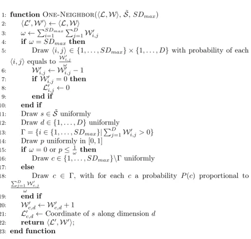
The function One-Neighbor() is given in Figure 2. First, it computes ω the total current model weight. Then operations carried out from lines 4 to 10 decrease the model weight when the total weight reaches the maximum model size (i.e., SDmax). This is performed by picking at random a pair of indices hi, ji with a probability proportional to Wi,j (line 5). Then the corresponding weight Wi,j is decreased (line 6). For the sake of clarity the associated coordinate Li,j is set to zero if Wi,j = 0 (line 8), even though this is not useful for the rest of the process. Next, the algorithm draws uniformly an object s in the sample and a dimension d in the space D (lines 11 and 12). Line 13 computes the set Γ of the indices of the valid centers. Then the algorithm chooses a random center
1: function One-Neighbor(hL, Wi, ˜S, SDmax)
2: hL0, W0i ← hL, Wi
3: ω ←PSDi=1maxPDj=1Wi,j0
4: if ω = SDmax then
5: Draw hi, ji ∈ {1, . . . , SDmax} × {1, . . . , D} with probability of each hi, ji equals to W 0 i,j ω 6: Wi,j0 ← Wi,j0 − 1 7: if Wi,j0 = 0 then 8: L0i,j← 0 9: end if 10: end if 11: Draw s ∈ ˜S uniformly 12: Draw d ∈ {1, . . . , D} uniformly 13: Γ = {i ∈ {1, . . . , SDmax}|P D j=1Wi,j0 > 0} 14: Draw p uniformly in [0, 1] 15: if ω = 0 or p ≤ ω1 then
16: Draw c ∈ {1, . . . , SDmax}\Γ uniformly
17: else
18: Draw c ∈ Γ, with for each c a probability P (c) proportional to
PD j=1W 0 c,j ω 19: end if 20: Wc,d0 ← Wc,d0 + 1
21: L0c,d← Coordinate of s along dimension d
22: return hL0, W0i;
23: end function
Figure 2: Generation of one neighbor.
15 and 16), or one of the current valid centers (line 18). In the latter case, the valid center is picked with a probability proportional to its total weight. Finally the weight Wc,dis increased and the location encoded in Lc,dis replaced by the coordinate of s along dimension d.
5.3
Complexity
Consider one iteration of SubCMedians using sample ˜S and let N bCenters
denote the number of centers currently used (the valid centers). It can be easily derived (see Appendix A.2) that the complexity of an iteration in SubCMedians
is then O(| ˜S| × N bCenters × D) and its memory requirement is simply O(D ×
6
Experimental Setup
6.1
Experimental protocol
The SubCMedians algorithm extends the subspace clustering tool family to-wards medians based clustering. Even if cluster center locations based on medi-ans can be interesting on their own (depending on the targeted task), an open question is to what extent the clusters obtained make sense with respect to those given by other paradigms? We used the evaluation framework of reference de-signed for subspace clustering described in [13] that reports the results obtained by well-established approaches for different evaluation measures, on both real and synthetic datasets. The method presented in [13] relies on a broad ex-ploration of the parameter space for each algorithm in order to find the best parameter setting on each data set and then compare the best results obtained by the different methods (see Appendix A.4). However such parameter tuning is most of the time a difficult task and these high quality subspace clustering models are likely to be difficult to obtain. For SubCMedians, for each dataset, a single parameter setting was used based on a default setting presented in Sec-tion 6.3. Since SubCMedians is nondeterministic (as many subspace clustering approaches), it can achieve different results on different runs. Consequently the algorithm was executed 10 times independently using the same parameter setting. The results obtained after each run were assessed with the same crite-ria as in [13]: the coverage, the number of clusters found, the average cluster
dimensionality and different quality measures (F1, accuracy, CE, RN IA and
entropy).
All experiments were run on an Intel 2.67GHz CPU running Linux Debian 8.3, using a single core and less than 150 MB of RAM. The SubCMedians algorithm has been implemented in C++ (as a Python library) and is available upon request.
6.2
Datasets
The performances of SubCMedians are reported on real world data using the seven benchmark datasets selected in [13] for their representativity: breast, di-abetes, liver, glass, shape, pendigits and vowel (most of them coming from the UCI archive [3]). These datasets have different dimensionalities and contain different numbers of objects. These objects are already structured in classes, and the class membership is used by quality measures to assess the cluster pu-rity. However, the number of classes does not necessarily reflect the number of subspace clusters, and the objects of a class can form different groups in space and/or strongly overlap with the objects of other classes.
SubCMedians was also executed on the 16 synthetic benchmark datasets provided by [13]. These datasets are particularly useful to study the algorithm performances, as the true clusters and their subspaces are known. Each dataset contains 10 hidden subspace clusters laying in subspaces made by 50%, 60% and 80% of the total dimensions of the dataset. Seven synthetic datasets allow
to study scalability with respect to the dataset dimensionality (5, 10, 15, 20, 25, 50 and 75 dimensions). These datasets contain about 1500 objects each and are extended with about 10% of noise objects. Five other synthetic datasets permit to analyse the scalability with respect to the dataset size (1500, 2500, 3500, 4500 and 5500 objects), over 20 dimensions, also with about 10% of noise objects. Finally four datasets allow to study the capacity to cope with noise, containing 10%, 30%, 50% and up to 70% of noise objects.
All datasets are made available by the authors of [13] at http://dme.rwth-aachen.de/openSubspace/evaluation. We applied a z-score standardization to all real and synthetic datasets in a preprocessing step.
6.3
Parameter values
The SubCMedians algorithm has three parameters: SDmax, N bIter, and N .
The most important is SDmax, the maximum model size, constraining the level
of detail of the subspace clustering performed. The number of iterations N bIter is also important but it should be noticed that its setting could be avoided since the user could monitor the value of the SAE during the clustering and stop the process when this value does no longer improve. The third one, the sample size N is a way to reduce the computing resources needed, and of course if possible it makes sense to use the full dataset instead of a sample.
In this section, we provide guidelines for easy default parameter setting. In this context, the user only needs to provide an expected or suggested number
of clusters N bExpClust. Let D denote the dimensionality of each
particu-lar dataset. The default setting is SDmax = N bExpClust × D, N bIter =
10 × SDmax× N bExpClust and N = 25 × N bExpClust (see Appendix A.3
for justification and technical details). For the synthetic datasets the num-ber of expected clusters is about 10, thus the maximum model size was set to
SDmax = D × 10, the sample size was set to N = 25 × 10 and the number
of iterations was set to N bIter = 10 × 10 × SDmax. A weaker setting, not
based on the true number of clusters, but based on 20 expected clusters, was also used, and as reported in Section 7 still permitted to exhibit structures of about 10 clusters. For the real world datasets, the only information available about the structure of the datasets is the number of classes. However, as al-ready mentioned, the number of classes may not correspond to the number of clusters. Indeed, according to the results provided by [13], in these datasets the state-of-the-art algorithms exhibit most of the time structures composed of more clusters than the number of classes. The setting of SubCMedians parameters is thus based on an expected number of clusters equal to three times the number of classes and we let the algorithm regulate itself the number of output clusters.
Hence the maximum model size was set to SDmax = 3 × N bClasses × D, the
sample size was set to N = 25 × 3 × N bClasses and the number of iterations
6.4
Evaluation measures
In order to compare our algorithm to the others, we used the same standard evaluation measures for clusters and subspace clusters as in [13]: entropy (the
normalized entropy), accuracy, F 1, RN IA and CE. We performed also the
same simple transformation on entropy and RN IA, by computing RN IA = 1 − RN IA and entropy = 1 − entropy to have all evaluation measures ranging from 0 (low quality) to 1 (high quality). The three first measures (entropy, accuracy and F 1) reflect how well objects that should have been grouped together were effectively grouped. The two last measures (RN IA and CE) take into account the way the objects are grouped and also the relevance of the subspaces found by the algorithm. For these measures, when the true dimensions of the subspace clusters were not known (for real datasets), then as in [13] all dimensions were considered as relevant, but then the interpretation of these two measures should remain cautious since the true sets of dimensions are likely to be smaller. Of course this does not apply to the synthetic datasets, since for them the reference clusters and their dimensions are known. We refer the reader to [13] for the detailed recall of the evaluation measures.
7
Experimental Results
Because of the large number of results (23 datasets and 11 algorithms) used in the comparison, aggregated figures reflecting the real detailed results are given. However, there is no ever winning paradigm or clustering method, each having its own advantages or interest.
7.1
Real dataset
This section presents the results obtained on the 7 representative real datasets selected in [13]. In order to assess if SubCMedians produced decent results with respect to well-established methods, we ranked the different methods with re-spect to their quality measures, their coverage (fraction of objects of the dataset that were grouped into clusters) and the number of clusters they produced (see Appendix A.5 for a detailed presentation of this procedure).
The average rank of each algorithm regarding the cluster quality measures, the coverage and the number of clusters found are given in Figure 3 (highest ranks meaning best results). In addition, two tables representative of the results at a more detailed level are presented in Figure 4. These tables report on two of the real world datasets the values for the coverage, the number of clusters found, their average dimensionality and the runtimes. Runtimes are given only as complementary information since for SubCMedians they were obtained on a computer (2.67GHz CPU) different from the one used by [13] (2.3GHz CPU). At the bottom of these tables, we grouped the results obtained by methods belonging to the same family as SubCMedians (clustering-oriented techniques), results for the other algorithms are provided for the sake of completeness.
1 2 3 4 5 6 7 8 9 10 11 12 Average quality rank
MINECLUS *SUBCMEDIANS DOC *PROCLUS INSCY *STATPC *P3C SCHISM CLIQUE SUBCLU FIRES 1 2 3 4 5 6 7 8 9 10 11 12 Average coverage rank
*SUBCMEDIANS CLIQUE SUBCLU MINECLUS SCHISM DOC *P3C *STATPC INSCY *PROCLUS FIRES 1 2 3 4 5 6 7 8 9 10 11 12 Average NbClusters rank
*P3C FIRES *PROCLUS *SUBCMEDIANS DOC *STATPC MINECLUS INSCY SUBCLU SCHISM CLIQUE
Figure 3: Average rankings over all datasets regarding the quality, the coverage and the number of clusters.
Figures 3 and 4 show evidence that the robustness of the medians still op-erates in this subspace clustering task since competitive cluster qualities can be obtained without discarding any object (100% coverage). In all experiments SubCMedians was run using the default parameter setting. For the number of clusters found, SubCMedians is above the average, and it seems that it does not tend to split the dataset into too many clusters. However, the true numbers of clusters are not known here, in contrast to the synthetic datasets.
7.2
Synthetic data
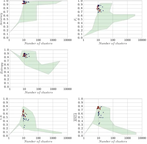
In this section, we report the results obtained on the 16 synthetic datasets of [13], each one containing 10 known clusters. For each dataset, SubCMedi-ans was executed 10 times and the model having the lowest SAE was retained (no use of external labeling). These models are depicted as red circles in Fig-ure 7 (blue triangles correspond to models obtained with an unweighted version of SubCMedians discussed here after). The green shapes represent the areas where are located the best models found by the 10 other algorithms over their parameter spaces (optimized using external ground truth labeling). Here again, the results show evidences that a median based approach is an interesting com-plementary tool for subspace clustering, and in particular that SubCMedians reaches a competitive quality for the measures that take into account not only the objects grouping, but also the dimensions associated to the clusters (RN IA and CE). Runtimes as functions of the size of the sample and the dimensional-ity of the dataset are provided in Figure 6. In these experiments the parameters where set according to the guidelines of Section 6.3 using an expected number
Pendigits: 16 dimensions, 10 classes, 7494 objects
Coverage Cluster N umber Average Dim Runtime (seconds) max min max min max min max min CLIQUE 1.00 1.00 1890.0 36.0 3.10 1.50 67891 219 DOC 0.91 0.91 15.0 15.0 5.50 5.50 178358 178358 MINECLUS 1.00 1.00 64.0 64.0 12.10 12.10 780167 692651 SCHISM 1.00 0.93 1092.0 290.0 10.10 3.40 500000000 21266 SUBCLU Runtime exceeding the maximal runtime allowed FIRES 0.94 0.94 27.0 27.0 2.50 2.50 169999 169999 INSCY 0.91 0.82 262.0 106.0 5.30 4.60 2000000 1000000 PROCLUS 0.90 0.74 37.0 17.0 14.00 8.00 6045 4250 P3C 0.90 0.90 31.0 31.0 9.00 9.00 2000000 2000000 STATPC 0.99 0.84 4109.0 56.0 16.00 16.00 50000000 3000000 SUBCMEDIANS 1.00 1.00 41.0 34.0 12.21 10.51 556 523
Diabetes: 8 dimensions, 2 classes, 768 objects
Coverage Cluster N umber Average Dim Runtime (seconds) max min max min max min max min CLIQUE 1.00 1.00 349.0 202.0 4.20 2.40 11953 203 DOC 1.00 0.93 64.0 17.0 8.00 5.10 1000000 51640 MINECLUS 0.99 0.96 39.0 3.0 6.00 5.20 3578 62 SCHISM 1.00 0.79 270.0 21.0 4.20 3.90 35468 250 SUBCLU 1.00 1.00 1601.0 325.0 4.70 4.00 190122 58718 FIRES 0.81 0.03 17.0 1.0 2.50 1.00 4234 360 INSCY 0.83 0.73 132.0 3.0 6.70 5.70 112093 33531 PROCLUS 0.92 0.78 9.0 3.0 8.00 6.00 360 109 P3C 0.97 0.88 2.0 1.0 7.00 2.00 656 141 STATPC 0.97 0.75 363.0 27.0 8.00 8.00 27749 4657 SUBCMEDIANS 1.00 1.00 16.0 13.0 3.69 2.87 3 3
Figure 4: Details of the cluster structures and of the runtimes on Pendigits and Diabetes.
of clusters of 10, but no constraint on the sizes of their subspaces. Interestingly, a weaker setting based on an expected number of clusters of 20 still permitted to SubCMedians to exhibit most of the time a good quality clustering of about 10 clusters (not shown, very similar to Figure 7).
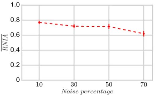
Figure 5 illustrates the clustering quality in terms of RN IA for increasing percentages of noise points in the dataset (respectively 10, 30, 50 and 70% of the data points were noise points). Even if the quality of the subspace clusters obtained tends to decrease when the amount of noise in the dataset increases,
the degradation is not severe. Here again, this seems to indicates that the
robustness to noise of the medians still operates in a subspace clustering task. In order to assess the impact of the weighted neighborhood exploration of the model space used by SubCMedians, the algorithm was compared to an unweighted version. In this version, the candidate center undergoing the mod-ification is uniformly drawn by modifying line 18 in Figure 2, and in the same
figure line 20 is replaced by Wc,d0 ← 1 to have weight matrices that contain
simply a 1 for a dimension that is used and a 0 otherwise.
The results of the more naïve unweighted version of SubCMedians are rep-resented in Figure 7 by blue triangles (same procedure used, retaining also the lowest SAE over 10 runs). The unweighted-SubCMedians outputted slightly more clusters than expected, and has another more important drawback, that is the lower quality obtained with respect to the dimensions found (RN IA
10 30 50 70 Noisepercentage 0 0.2 0.4 0.6 0.8 1.0
R
N
IA
Figure 5: Mean RN IA vs percentage of noise points in the dataset.
and CE graphics). As targeted by the design of the neighborhood
explo-ration in Section 5, the weighted strategy of SubCMedians could focus on more promising clusters while unweighted-SubCMedians produced more (use-less) candidate centers (Figure 8) and failed to develop sufficiently the center dimensionalities when the hidden cluster dimensionalities increased (Figure 9). Moreover, SubCMedians turned out to be slightly faster (see Figure 6), and unweighted-SubCMedians suffered from a small overhead likely to be caused by its handling of more candidate centers in the models.
8
Conclusion
In this paper we presented SubCMedians, a median-based subspace clustering method, and assessed it on real and synthetic benchmark datasets, using the evaluation framework of [13]. These results showed that a median-based sub-space clustering approach can exhibit satisfactory results when compared to well-established subspace clustering paradigms, and is thus a good candidate as a complementary tool, in particular for users interested by the properties of medians themselves (facility location, robustness to noise and outliers). We also proposed some guidelines for easy default parameter setting. These guidelines were effective when dealing with all the datasets of the benchmark. Since the median-based subspace clusters seem to be obtained in rather short runtimes, promising future work includes the use of these clusters as initial guesses to guide other techniques that could be more time consuming.
A
Appendix
A.1
Expected gain in SAE to guide local exploration
Consider a cluster C and a dimension d. Let us suppose that the coordinates Xdof the objects in C along d follow a Gaussian distribution N (µd, σd). Let us consider that a badly placed center m is simply an object in C taken randomly. Along dimension d, the difference between the location of an object X chosen
0 500 1000 1500
Sample
size
0.1 1 10 100 1000R
un
ti
m
e
(se
co
nd
s
)(a) Runtime vs. dataset sample size.
5 10 15 20 25 50 75
Dataset
dimensionality
0.1 1 10 100 1000R
un
ti
m
e
(se
co
nd
s
)(b) Runtime vs. dataset dimensionality
Figure 6: Runtimes (avg. 10 runs) for SubCMedians vs sample sizes (| ˜S|) for the synthetic dataset of size 5500 (6a), and vs the synthetic dataset dimensionalities (6b). Runtimes of the unweighted version of SubCMedians as blue triangles.
1 10 100 1000 10000 Numberofclusters 0.0 0.1 0.2 0.3 0.4 0.5 0.6 0.7 0.8 0.9 1.0
A
cc
ur
ac
y
1 10 100 1000 10000 Numberofclusters 0.0 0.1 0.2 0.3 0.4 0.5 0.6 0.7 0.8 0.9 1.0F
1 1 10 100 1000 10000 Numberofclusters 0.0 0.1 0.2 0.3 0.4 0.5 0.6 0.7 0.8 0.9 1.0E
nt
ro
py
1 10 100 1000 10000 Numberofclusters 0.0 0.1 0.2 0.3 0.4 0.5 0.6 0.7 0.8 0.9 1.0CE
1 10 100 1000 10000 Numberofclusters 0.0 0.1 0.2 0.3 0.4 0.5 0.6 0.7 0.8 0.9 1.0R
N
IA
Figure 7: Quality measures and number of clusters obtained on synthetic
datasets by SubCMedians (red circles) and the other algorithms (green areas). Results of the unweighted version of SubCMedians as blue triangles.
randomly in C and the location of m, is (Xd− md) and follows the distribution N (µ0
d, σd0) with µ0d= 0 and σ0d= σd √
2 since Xd and md follows N (µd, σd).
Let us consider that a well placed center m∗is the median of the n objects
of C contained in the current sample ˜S. Using the distribution followed by such a median estimator and obtained in Section 4.2 we have m∗ ∼ N (µd, σdp2nπ). Thus the difference between the locations of object X and m∗along d, (Xd−m∗d), follows the distribution N (µ∗d, σd∗) with µ∗d= 0 and σd∗= σd
pπ
2n + 1.
For m the contribution of X to the AE value (and thus to SAE) is |Xd−
md|. As (Xd− md) ∼ N (µ0d, σ 0
d), then |Xd− md| follows the corresponding
folded normal distribution and the expected value of |Xd − md| is given by
σd0p2/π exp(−µ02d/2σd02) + µ0d[1 − 2Φ(−µ0d/σd0)], where Φ denotes the normal cumulative distribution. Since µ0d= 0 and σd0 = σd
√
2, we have E(|Xd− md|) = 2σd/
√
π. In a similar way we can derive the expected value of the contribution of X to AE for the optimized center m∗, E(|Xd− m∗d|) = σd
q 1
n +
2
π.
If we consider γ = E(|Xd− m∗d|) − E(|Xd− md|) as reflecting the gain due in the optimized case, then γ = σd(2/
√
π −q1n+π2). This means that larger
gains are likely to be obtained for clusters having a high σd and having many
of their elements belonging to the sample ˜S.
A.2
Complexity
Consider one iteration of SubCMedians using sample ˜S in a D dimensional
space. Let N bCenters denote the number of centers currently used (the valid centers). Operations in non-constant time are the calls to AE, SAE and One-Neighbor(). AE computes the distance of one object to each center and is in O(N bCenters × D). SAE does the same for each object in the sample and
then has a complexity O(| ˜S| × N bCenters × D). The computation cost of
One-Neighbor() lies in part in the computation of weights: the total weight of the model ω (line 3) and the weights in the probabilities used line 18. These values can be maintained incrementally when W is modified resulting in a constant cost for ω and in a cost proportional to N bCenters for the probabilities line
18. The remaining cost is due to the non-uniform random selections (lines
5 and 18), having a cost proportional to the number of possible outcomes. Line 5 there are at most N bCenters × D possible outcomes with a non-zero probability (other pairs hi, ji having a weight of zero). And for line 18 there are N bCenters possible outcomes. The cost of one call to One-Neighbor() is thus in O(N bCenters × D). The complexity of an iteration in SubCMedians is then O(| ˜S| × N bCenters × D).
The memory requirement of one iteration of SubCMedians corresponds to
the storage of the sample ˜S and the two matrices L and W of size SDmax× D
A.3
Parameter Setting
The easy default parameter setting (for preliminary exploration of the data) re-quires to provide only one value: the expected number of clusters N bExpClust. Notice that this is not a crisp constraint, but only a suggested number of clus-ters that the algorithm should adjust to build a structure. Notice also that a hard part of the subspace clustering task is to determine the subspaces and that this aspect is not directly constrained by N bExpClust.
Maximum model size SDmax The intuition to set SDmax is very simple,
the value of SDmax should allow to build a model containing N bExpClust
even if all dimensions are useful, leading to a default SDmax value equal to
N bExpClust × D. Of course, as for any subspace clustering algorithm, obtain-ing very satisfactory results are likely to require from the user finer parameter tuning.
From N bExpClust and SDmax we now derive minimum recommended
val-ues for the number of iterations and for the sample size. These settings are the ones used in the experiments reported Section 7, but of course the statistical thresholds used in the setting method could be enforced in order to have more conservative recommended parameter values.
Number of iterations N bIter Let C be any expected cluster and d be any
of its dimensions. Let k be the number of attempts to set the coordinate of the center of C along d to a reasonable approximation of the median value, during N bIter iterations in SubCMedians. The default value proposed for N bIter is the minimum number of iterations such that the expected value of k is at least 1.
Let us suppose that all clusters have the same size and that the number of clusters is equal to N bExpClust. Consider an iteration of SubCMedians. In One-Neighbor() (Figure 2) the probability to pick an object s belonging to C (line 11) is 1/N bExpClust and the probability to choose dimension d (line 12) is 1/D. Let x be the coordinate of s along dimension d, and let us accept as a reasonable approximation a value x at a distance of less than 1/8 of the standard deviation away from the median. Then, supposing a Gaussian distribution, this implies that the median is equal to the mean, and that the probability of x as being a reasonable approximation is about 0.1 (according to the standard normal cumulative distribution). At line 15, the probability to jump to line 18 to modify an existing cluster is 1 − 1/ω. If we suppose that the current model contains already N bExpClust clusters, including C (possibly with the presence of a single dimension of C), and that all clusters have similar weights in matrix W, then the probability of C to be chosen in line 18 is about 1/N bExpClust. So the probability p of the center corresponding to C in the current model, to have its coordinate along dimension d to be set to a reasonable approximation x in line 21, is p = N bExpClust1 × 1 D× 0.1 × (1 − 1 ω) × 1 N bExpClust. As ω increases
at each iteration (up to SDmax) we quickly have (1 −ω1) ' 1, and since we set
SDmax= N bExpClust × D, we have p ' 0.1 ×SD 1
The expected value of k is E(k) = N bIter × p, thus to have E(k) ≥ 1, the
default minimum N bIter value is set to 10 × SDmax× N bExpClust.
Dataset sample size N Consider a cluster C and a dimension d, supposing
that the coordinates in C along d follow N (µd, σd). As stated in Section 4.2, ˆ
θd the median estimator of these coordinates, using a sample of size n, follows N (µd, σdp2nπ). If we accept a standard error of 1/4 of the original σd then the minimum sample size satisfies σθˆ
d =
σd
4 = σd
pπ
2n and we have n = 8π '
25. Such sample allows to estimate the median location of a cluster in the D dimensions, but if there are N bExpClust clusters, more objects are needed. Let us suppose that all clusters have the same size, and thus are likely to be represented by similar numbers of objects in the sample, then the recommended minimum value for N is 25 × N bExpClust.
A.4
Evaluation framework
The evaluation framework of [13] relies on a systematic approach to compare the results of representative algorithms that address the major subspace clustering paradigms. The comparison detailed in [13] was made using different evaluation measures on both real and synthetic datasets, using the following method. Given that each algorithm requires several parameters (from 2 to 9), for each dataset, the algorithms were executed with 100 different parameter settings to explore the parameter space. Then, using an external labeling of the objects, only the outputs that were among the best with respect to the external labeling (taken as a ground truth) were retained. So, the results reported in [13] are in some sense the best possible subspace clusterings that could be achieved if we were able to find the most appropriate parameter values. More precisely, for each real world dataset only two outputs were retained: 1) the one computed for
the parameter setting that maximizes the F1 measure, and 2) the one obtained
when maximizing the accuracy. These two outputs led to two values for each measure, the smallest of the two being called bestMin and the other bestMax. For each synthetic dataset, all the settings maximizing at least one quality
measures among F1, accuracy, CE, RN IA and entropy were retained. bestMin
and bestMax are reported as min and max in Figure 4.
Since generally no external labeling is available when we search for clus-ters, parameter tuning is most of the time a difficult task and these high quality subspace clustering models are likely to be hard to obtain. Instead, for SubCMe-dians, the parameters were not optimized using any external criteria and were set to the default values suggested in Section A.3. For each real world dataset, the highest and lowest values of each evaluation measure over 10 runs were com-puted, so as to compare them to the bestMax and bestMin values retained by the evaluation method of [13]. For each synthetic dataset, we simply took the clustering having the lowest SAE measure (internal criterion of quality).
0 10 20 30 40 50 60 70 80 Datasetdimensionality 0 50 100 150 200 250 300 350 400
N
um
be
r
of
ca
nd
id
at
e
ce
nt
er
s
Figure 8: Number of candidate centers (avg. 10 runs) for SubCMedians (red circles) and unweighted-SubCMedians (blue triangles) vs dataset dimensionality.
A.5
Ranking method over real world datasets
The algorithms were ranked over the seven real world datasets using the follow-ing procedure.
Cluster quality measures For each measure, on each data set, two rankings
of the 11 algorithms were computed: one for the bestM ax score and one for the bestM in score (see Appendix A.4), with ranks ranging from 1 to 11, rank 11 being associated to the algorithm obtaining the highest quality. The overall ranking of an algorithm was then simply the average of its rank values.
Coverage The same procedure was used to compare the coverages obtained.
The coverage denotes the fraction of objects of the dataset that are associated to clusters. This measure is less than 1 if some objects are not associated to one of the output clusters, or if they are identified as outliers or as reflecting noise. When the coverage decreases, discarding some objects can result in a direct improvement of several quality measures (because of clusters being more homogeneous). Of course putting apart too many objects is likely to lead to less representative models and is most of the time not desirable. For the coverage a rank value of 11 was associated to the highest coverage.
Number of clusters The rankings were computed using the absolute value
of the difference between the number of clusters found by the algorithm and the number of classes in the dataset. The rank value 11 is given to the smallest absolute value. However, as previously mentioned, the number of classes does not necessarily reflect the number of subspace clusters in the datasets.
The global trade-off is then to reach high quality measures while preserving a high coverage (except for data containing many outliers or important noise), and without splitting the data into too many clusters.
0 10 20 30 40 50 60
Meanhiddenclusterdimensionality
0 10 20 30 40 50 60
M
ea
n
ce
nt
er
di
m
en
si
on
al
ity
Figure 9: Subspace mean size of the centers (avg. 10 runs) for SubCMedians (red circles) and unweighted-SubCMedians (blue triangles) vs subspace mean size of the hidden clusters.
B
Acknowledgements
This research has been supported by EU-FET grant EvoEvo (ICT-610427). Other support: Christophe Rigotti is a member of LabEx IMU (ANR-10-LABX-0088).
References
[1] C. C. Aggarwal, A. Hinneburg, and D. A. Keim. On the surprising behavior of distance metrics in high dimensional space. In Proc. of ICDT, pages 420–434, 2001.
[2] C. C. Aggarwal, J. L. Wolf, P. S. Yu, C. Procopiuc, and J. S. Park. Fast algorithms for projected clustering. In Proc. of ACM SIGMOD, pages 61–72, 1999.
[3] K. Bache and M. Lichman. UCI machine learning repository, 2013.
[4] S. Har-Peled and A. Kushal. Smaller coresets for K-median and K-means clus-tering. Discrete & Computational Geometry, 37(1):3–19, 2006.
[5] K. Jain and V. V. Vazirani. Approximation algorithms for metric facility location and K-median problems using the primal-dual schema and lagrangian relaxation. Journ. of ACM, 48(2):274–296, 2001.
[6] M. Jamshidi. Median location problem. In R. Zanjirani Farahani and M. Hekmat-far, editors, Facility Location: Concepts, Models, Algorithms and Case Studies, pages 177–191. Physica-Verlag, 2009.
[7] H.-P. Kriegel, P. Kröger, and A. Zimek. Clustering high-dimensional data: A sur-vey on subspace clustering, pattern-based clustering, and correlation clustering. ACM TKDD, 3(1):1–58, 2009.
[8] H.-P. Kriegel, P. Kröger, and A. Zimek. Subspace clustering. Wiley Interdisci-plinary Reviews: Data Mining and Knowledge Discovery, 2(4):351–364, 2012. [9] K. H. Lim, L. Ferraris, M. E. Filloux, B. J. Raphael, and W. G. Fairbrother.
Using positional distribution to identify splicing elements and predict pre-mrna processing defects in human genes. Proc. of the National Academy of Sciences, 108(27):11093–11098, 2011.
[10] Y. Liu, L. C. Jiao, and F. Shang. An efficient matrix factorization based low-rank representation for subspace clustering. Pattern Recognition, 46(1):284–292, 2013. [11] J. S. Maritz and R. G. Jarrett. A note on estimating the variance of the sample median. Journ. of the American Statistical Association, 73(361):194–196, 1978. [12] R. Maronna, D. Martin, and V. Yohai. Robust statistics. John Wiley & Sons,
2006.
[13] E. Müller, S. Günnemann, I. Assent, and T. Seidl. Evaluating clustering in subspace projections of high dimensional data. In Proc. of VLDB, pages 1270– 1281, 2009.
[14] L. Parsons, E. Haque, and H. Liu. Subspace clustering for high dimensional data: A review. ACM SIGKDD Explorations Newsletter, 6(1):90–105, 2004.
[15] G. Sen, M. Krishnamoorthy, N. Rangaraj, and V. Narayanan. Exact approaches for static data segment allocation problem in an information network. Computers & Operations Research, 62:282–295, 2015.
[16] S. J. Sheather. A finite sample estimate of the variance of the sample median. Statistics & Probability Letters, 4(6):337–342, 1986.
[17] K. Sim, V. Gopalkrishnan, A. Zimek, and G. Cong. A survey on enhanced sub-space clustering. DMKD, 26(2):332–397, 2013.
[18] Y. Wang and J. Zhu. Dp-space: Bayesian nonparametric subspace clustering with small-variance asymptotics. In Proc. of ICML, pages 1–9, 2015.