d’hypergraphes
Fault-tolerant gates on hypergraph product codes
par
Anirudh Krishna
Thèse présentée au département de physique
en vue de l’obtention du grade de docteur ès sciences (Ph.D.)
FACULTÉ des SCIENCES UNIVERSITÉ de SHERBROOKE
Le 31 Janvier 2020
le jury a accepté la thèse de Monsieur Anirudh Krishna dans sa version finale.
Membres du jury
Professeur David Poulin Directeur de recherche Département de physique
Professeur Louis Taillefer Membre interne Département de physique
Professeur Robert Koenig Membre externe
Département de Mathematique Technische Universität München
Professeur Ion Garate Président-rapporteur Département de physique
Sommaire
L’un des défis les plus passionnants auquel nous sommes confrontés aujourd’hui est la perspective de la construction d’un ordinateur quantique de grande échelle. L’information quantique est fragile et les implémentations de circuits quantiques sont imparfaites et su-jettes aux erreurs. Pour réaliser un tel ordinateur, nous devons construire des circuits quan-tiques tolérants aux fautes capables d’opérer dans le monde réel. Comme il sera expliqué plus loin, les circuits quantiques tolérant aux fautes nécessitent plus de ressources que leurs équivalents idéaux, sans bruit.
De manière générale, le but de mes recherches est de minimiser les ressources nécessaires à la construction d’un circuit quantique fiable. Les codes de correction d’erreur quantiques protègent l’information des erreurs en l’encodant de manière redondante dans plusieurs qubits. Bien que la redondance requière un plus grand nombre de qubits, ces qubits supplé-mentaires jouent un rôle de protection: cette redondance sert de garantie. Si certains qubits sont endommagés en raison d’un circuit défectueux, nous pourrons toujours récupérer l’informations.
Préparer et maintenir des qubits pendant des durées suffisamment longues pour effectuer un calcul s’est révélé être une tâche expérimentale difficile. Il existe un écart important entre le nombre de qubits que nous pouvons contrôler en laboratoire et le nombre requis pour implementer des algorithmes dans lesquels les ordinateurs quantiques ont le dessus sur ceux classiques. Par conséquent, si nous voulons contourner ce problème et réaliser des circuits quantiques à tolérance aux fautes, nous devons rendre nos constructions aussi ef-ficaces que possible. Nous devons minimiser le surcoût, défini comme le nombre de qubits physiques nécessaires pour construire un qubit logique. Dans un article important, Gottes-man a montré que, si certains types de codes de correction d’erreur quantique existaient, cela pourrait alors conduire à la construction de circuits quantiques tolérants aux fautes avec un surcoût favorable. Ces codes sont appelés codes éparses.
La proposition de Gottesman décrivait des techniques pour exécuter des opérations logiques iii
sur des codes éparses quantiques arbitraires. Cette proposition était limitée à certains égards, car elle ne permettait d’exécuter qu’un nombre constant de portes logiques par unité de temps. Dans cette thèse, nous travaillons avec une classe spécifique de codes éparses quantiques appelés codes de produits d’hypergraphes. Nous montrons comment effectuer des opérations sur ces codes en utilisant une technique appelée déformation du code. Notre technique généralise les codages basés sur les défauts topologiques dans les codes de surface aux codes de produits d’hypergraphes. Nous généralisons la notion de perforation et montrons qu’elle peut être exprimée naturellement dans les codes de pro-duits d’hypergraphes. Comme cela sera expliqué en détail, les défauts de perforation ont eux-mêmes une portée limitée. Pour réaliser une classe de portes plus large, nous intro-duisons un nouveau défaut appelé trou de ver basé sur les perforations. À titre d’exemple, nous illustrons le fonctionnement de ce défaut dans le contexte du code de surface. Ce défaut a quelques caractéristiques clés. Premièrement, il préserve la propriété éparses du code au cours de la déformation, contrairement à une approche naïve qui ne garantie pas cette propriété. Deuxièmement, il généralise de manière simple les codes de produits d’hypergraphes. Il s’agit du premier cadre suffisamment riche pour décrire les portes tolérantes aux fautes de cette classe de codes. Enfin, nous contournons une limitation de l’approche de Gottesman qui ne permettait d’effectuer qu’un certain nombre de portes logiques à un moment donné. Notre proposition permet d’opérer sur tous les qubits en-codés à tout moment.
Summary
One of the most exciting challenges that faces us today is the prospect of building a scal-able quantum computer. Implementations of quantum circuits are imperfect and prone to error. In order to realize a scalable quantum computer, we need to construct fault-tolerant quantum circuits capable of working in the real world. As will be explained further below, fault-tolerant quantum circuits require more resources than their ideal, noise-free counter-parts.
Broadly, the aim of my research is to minimize the resources required to construct a reli-able quantum circuit. Quantum error correcting codes protect information from errors by encoding our information redundantly into qubits. Although the number of qubits that we require increases, this redundancy serves as a buffer – in the event that some qubits are damaged because of a faulty circuit, we will still be able to recover our information. Preparing and maintaining qubits for durations long enough to perform a computation has proved to be a challenging experimental task. There is a large gap between the number of qubits we can control in the lab and the number required to implement algorithms where quantum computers have the upper hand over classical ones. Therefore, if we want to circumvent this bottleneck, we need to make fault-tolerant quantum circuits as efficient as possible. To be precise, we need to minimize the overhead, defined as the number of physical qubits required to construct a logical qubit. In an important paper, Gottesman showed that if certain kinds of quantum error correcting codes were to exist, then this could lead to constructions of fault-tolerant quantum circuits with favorable overhead. These codes are called quantum Low-Density Parity-Check (LDPC) codes.
Gottesman’s proposal described techniques to perform gates on generic quantum LDPC codes. This proposal limited the number of logical gates that could be performed at any given time. In this thesis, we work with a specific class of quantum LDPC codes called hypergraph product codes. We demonstrate how to perform gates on these codes using a technique called code deformation. Our technique generalizes defect-based encodings in
the surface code to hypergraph product codes. We generalize puncture defects and show that they can be expressed naturally in hypergraph product codes. As will be explained in detail, puncture defects are themselves limited in scope; they only permit a limited set of gates. To perform a larger class of gates, we introduce a novel defect called a wormhole that is based on punctures. As an example, we illustrate how this defect works in the context of the surface code.
This defect has a few key features. First, it preserves the LDPC property of the code over the course of code deformation. At the outset, this property was not guaranteed. Second, it generalizes in a straightforward way to hypergraph product codes. This is the first frame-work that is rich enough to describe fault-tolerant gates on this class of codes. Finally, we circumvent a limitation in Gottesman’s approach which only allowed a limited number of logical gates at any given time. Our proposal allows to access the entire code block at any given time.
Acknowledgements
I am extremely fortunate to have had the chance to work with David Poulin as a Ph.D. student. David is a role model both as researcher and adviser. His expertise in a wide range of topics, and interest in both concrete and abstract problems is an inspiration. In addition, David has been patient, kind and generous. I would like to express my sincerest thanks to David for this opportunity.
Inria was my home-away-from-home for a significant duration of my studies. I would like to thank Pierre Tillich for his guidance during my internship at Inria. Thanks to Jean-Pierre, I gained a special appreciation for classical coding theory. Jean-Pierre’s attention to detail also helped me write better.
My path down quantum error correction started with an internship with Daniel Gottesman. My interest in quantum LDPC codes began over lunch time conversations with Daniel at the Blackhole bistro at Perimeter. I’d like to thank Daniel for introducing me to one of the topics that became the focus of my Ph.D.
I’d like to thank Barbara Terhal and Alexandre Blais for inviting me to collaborate with their groups. I learned a lot working on these projects and this helped guide the course of my research. I’d also to like to thank Stephen Bartlett, Steve Flammia, and Ken Brown for inviting me to visit. Each of these visits were impactful, and I enjoyed discussions with you.
Over the past few years, I’ve had the opportunity to collaborate with inspiring people around the world. My Ph.D. wouldn’t have been the same without Nikolas Breuckmann, Christophe Vuillot, Ben Criger; Anthony Leverrier, Antoine Grospellier, Vivien Londe; Tomas Jochym O’Connor; Markus Kesselring; Narayanan Rengaswamy, and Mike Newman. I’ve learned a lot from all of you.
Sherbooke has been my home for the past three years and it wouldn’t have been complete without the team at Sherbrooke who served as friends and counsel. Thank you to Pavithran
Iyer, Andrew Darmawan, Guillaume Dauphinais, Colin Trout, Jessica Lemieux, Maxime Tremblay, Benjamin Bourassa, Yehua Liu, Shruti Puri, Jonathan Gross, Thomas Gobeil and Thomas Baker.
Outside my work environment, I’d like to thank Zoe Xuan Qin for bringing energy and happiness to my life. I would also like to thank Jalaj Upadhyay for being a friend and mentor.
Finally, none of this would have been possible without my family. My parents have been pillars of support, and my brother has been my North star. Regardless of what endeavor I had chosen to pursue, I couldn’t have done it without your support. Thank you.
Contents
Sommaire ii
Summary iv
Introduction 1
1 Classical Error Correction 5
1.1 Classical error correction . . . 5
1.2 Expander codes . . . 8
1.3 Chapter summary . . . 16
2 Quantum Error Correction 18 2.1 Quantum error correction . . . 19
2.2 CSS codes . . . 22
2.3 Universal gate sets . . . 24
2.4 Transversal gates . . . 25
2.5 State injection . . . 26
2.5.1 Magic state distillation . . . 27
2.6 Chapter Summary. . . 29
3 The Surface Code 30 3.1 Definition . . . 31
3.2 Decoding the surface code . . . 35
3.3 Defects on the surface code . . . 38
3.4 Clifford gates . . . 45
3.4.1 Measurements . . . 46
3.4.2 Resource state preparation . . . 50
3.5 Chapter summary . . . 51
4 Hypergraph Product Codes 53
4.1 Background and notation . . . 55
4.1.1 Classical and quantum codes . . . 55
4.1.2 The hypergraph product code. . . 56
4.2 The small-set-flip algorithm . . . 59
4.3 Chapter summary . . . 64
5 Defects on Hypergraph Product Codes 65 5.1 Punctures . . . 66
5.1.1 Definition . . . 66
5.1.2 Logical Pauli operators for punctures . . . 70
5.2 Wormholes . . . 79
5.2.1 Measurements and hybrid stabilizers . . . 81
5.2.2 Logical Pauli operators for wormholes . . . 84
5.3 Code deformation . . . 87
5.3.1 Non-mixing . . . 87
5.3.2 Code deformation on the hypergraph product code . . . 91
5.3.3 Measurements and traceability . . . 92
5.3.4 Resource states . . . 94
5.3.5 Point-like punctures . . . 96
5.4 Chapter summary . . . 98
Conclusion 99
List of Tables
5.1 Summary of properties of punctures.. . . 70
1.1 Factor graph of the repetition code. . . 9
1.2 Schematic of a factor graph . . . 11
2.1 Quantum codes via the CSS construction. . . 23
2.2 Error propagation in a circuit. . . 25
2.3 State injection . . . 27
3.1 The surface code. . . 32
3.2 X stabilizers of the surface code. . . 33
3.3 Stabilizers of the surface code. . . 34
3.4 Logical operators of the surface code. . . 35
3.5 Errors, stabilizers and logical operators on the surface code. . . 35
3.6 Half a stabilizer confounds a local decoder. . . 36
3.7 Illustrating minimum weight matching. . . 37
3.8 Smooth punctures. . . 40
3.9 Rough punctures. . . 41
3.10 Encoding logical qubits in punctures. . . 42
3.11 Braiding punctures on the surface code. . . 42
3.12 Creating a wormhole.. . . 43
3.13 Lattice-free representation of wormhole. . . 44
3.14 Stabilizer and logical generators of the wormhole. . . 45
3.15 A measurement-based circuit to perform controlled-Z. . . 46
3.16 The braiding operation.. . . 47
3.17 The stitching operation. . . 48
3.18 The Y operator of a wormhole is not traceable. . . 49
3.19 A product of Y operators of the wormhole are traceable.. . . 50
4.1 flipfails on hypergraph product codes. . . 59
4.2 Results of simulation of 5, 6 codes. . . 63
List of Figures xiii
5.1 Schematic of factor graphs.. . . 67
5.2 Schematic for a puncture on a hypergraph product code. . . 68
5.3 Panels(a)and(b)feature a smooth puncture defined on a lattice with only smooth boundaries. The strings of X operators defined only on VV qubits (as in panel(a)) or only on CC qubits (as in panel(b)) are equivalent. Panels(c)
and(d)feature a lattice with smooth and rough boundaries, with a smooth punctured carved out from the inside. The logical X shown running from the smooth puncture to the boundary in panels(c)and(d)are equivalent up to an embedded logical X. . . 77
5.4 Schematic for a wormhole on hypergraph product codes. . . 81
5.5 A pair of punctures used to encode a single logical qubit on the surface code. 90
5.6 A measurement-based circuit to perform controlled-Z. . . 91
5.7 A puncture crossing its own path. . . 94
The last decade has witnessed tremendous progress in quantum computation. Quantum computers may be capable of solving certain kinds of problems faster than their classical counterparts. However, we are still far from these applications as constructing a quantum computer is an enormously difficult problem. Quantum information is plagued by noise which impedes our ability to prepare and coherently maintain quantum bits (qubits). The domain of quantum error correction and fault tolerance emerged as a response to this prob-lem and forms a pillar of research in quantum computation.
The article [1] presents the accuracy of one- and two-qubit gates in some devices (see table 1 in [1]). Even with the smallest error rate of 0.01% reported in table 1, a quantum algorithm containing more than 10, 000 logical gates would very likely contain an error. More gener-ally, if the probability of failure of a circuit component is a constant, we are certain to fail as we build larger and larger circuits. Each architecture comes with its own set of advantages and disadvantages. The physical incarnation of the error mechanisms will depend on the experimental system in question. At this early stage, it is difficult to bet on one approach. For this reason, our discussion will abstract away the specifics of particular architectures. Although the actual values will change, errors are not something that will entirely be re-moved from our systems. It is highly unlikely that we will ever be able to engineer systems to the degree of precision required to run long quantum algorithms on raw qubits. This is disheartening because it seems to imply that quantum computation is impossible.
Quantum error correction is a software method used to construct arbitrarily accurate vir-tual qubits from underlying faulty physical qubits. In addition to error correction, a quan-tum computer must also manipulate the encoded information, and these logical operations must be executed in a way that avoids error propagation. The threshold theorem guarantees that as long as the probability that a circuit component fails is below some threshold, we can increase the length of the circuit arbitrarily [2,3,4,5,6]. At the heart of the threshold theorem are objects called error correcting codes. Error correcting codes are ways of storing
2
information redundantly and we shall review them in chapter2. This redundancy serves as a buffer – in the event that some physical qubits are corrupted, we can still retrieve the information. Once information is encoded in an error correcting code, we cannot point to any one region and ask if the information resides there. Rather, information is stored in non-local degrees of freedom in such a way that no local read-out can discern the encoded information. By the same token, local errors cannot damage stored information. However making systems robust comes at a cost of increasing the number of qubits we have to con-trol.
Optimizing the storage capacity of quantum error correcting codes is one way to minimize the qubits we need to perform quantum computation. The other concern is the number of extra qubits we need to perform measurements. In addition to the qubits required for storage, we also need extra qubits, i.e. an ancillary system, for performing measurements. Quantum error correcting codes necessitate performing joint measurements on sets of data qubits. Based on the outcome of these measurements, we can deduce the error and thereby perform error correction. The size of this ancilla system could grow considerably based on the technique that we use. These trade-offs will depend on the quantum error correcting code we choose.
Not all quantum error correcting codes are created equal. Some codes offer better protec-tion than others for fixed cost (as measured by figures of merit we shall discuss later). They also permit simple measurement protocols.
Raussendorf and collaborators [7,8,9] discovered a fault-tolerant scheme that is naturally defined by local interactions in a two-dimensional geometry and has a relatively large error threshold. In this scheme, logical qubits are encoded in Kitaev’s surface code [10,11] and some logical gates can be implemented by topologically protected operations. Another ad-vantage of the surface code is that performing joint measurements on the data qubits can be done using only a constant number of ancilla qubits. This topological architecture has been the object of intense theoretical studies and is now being pursued by major experimen-tal groups and corporations worldwide (see for example [12,13] and references contained therein). We shall cover these properties in chapter3. Experimental demonstrations of fault tolerance will certainly be a milestone experiment in the next few years. The success of the surface code architecture can on the one hand largely be attributed to its simplicity and rel-atively good performance, but on the other hand this architecture has benefited from over a decade of theoretical development and optimization. In fact, this single architecture has probably received far more theoretical inputs than all other coding schemes combined, so it should not come as a surprise that it has caught the attention of experimentalists.
It is unclear that the surface code will be the architecture we choose to use in the long run. The article [14] shows resource estimates for implementing Shor’s algorithm using the surface code (see table 1 in [14]). We can see that even with optimistic assumptions, it will take anywhere between a million and hundred million physical qubits to run the algorithm in a year. When we struggle to control tens of qubits today, these numbers do not appear to be in the realm of the attainable. However we could also interpret these numbers to mean that the surface code is perhaps not the best architecture suited for scalable quantum computation. What class of codes can replace the surface code while maintaining some or all of the features that make it appealing? Does there exist another local code capable of storing more logical qubits and simultaneously able to protect qubits just as well?
Unfortunately, all quantum error correcting codes that can be laid out on a table top with only nearest neighbor connections are limited by construction. Results like [15,16] place severe restrictions on local quantum error correcting codes. If we wish to increase the ca-pacity of quantum error correcting codes, something has to give.
Motivated by this state of affairs, this thesis will emphasize one particular alternative to the surface code, namely quantum Low-Density Parity-Check (LDPC) codes. Although we will discuss the surface code to help build intuition for LDPC codes, this thesis is not a review of the surface code. For a review of quantum error correction from a different perspective, see [17]. The main similarity between the surface code and LDPC codes is that error correction requires only joint measurement on a sparse set of qubits, hence the name. This is an important feature because the experimental complexity of performing multi-qubit measurements generally scales with the number of involved qubits, so it is desirable to keep that number low. In addition to this sparsity constraint, the measurements in the surface code only involve qubits which are geometrically near each other, and this restriction is dropped in more general LDPC codes.
The upshot of this relaxation is a lower encoding overhead: much fewer physical qubits are needed to encode a given number of logical qubits to some desired logical accuracy. This is a very desirable feature, but it comes at the cost of using non-local multi-qubit measurements. While this is experimentally very challenging, an in-depth study of the benefits of LDPC codes is needed before deciding if they are worth the additional experimental efforts. This thesis is a step in that direction.
Once quantum information has been encoded in an error correcting code, we need to find ways of manipulating this information to perform computation. These operations must be performed such that in the event of an error on one qubit, the operations do not spread the error to other qubits. Such an avalanche of errors would be disastrous as the quantum
4
error correcting code can only buffer against a limited number of errors. Thus we seek to perform gate operations in a fault-tolerant manner. We could approach this in many ways. For instance, one way to do so would be to directly perform the unitary gate on the error correcting code. If these gates can be implemented in a short duration, it minimizes the amount of time available for potential errors to propagate to many qubits. Whether or not such gates exist depends on the quantum error correcting code, and symmetries it may possess. We shall say more about such codes in chapter2.
Rather than take this approach, we shall use a framework called code deformation. Code deformation involves modifying the code gradually and this transformation eventually re-turns to the code that we started with. The aim is for this sequence of gradual transfor-mations to have a non-trivial logical effect on the code. We present the first framework to perform fault-tolerant gates on quantum LDPC codes. We shall focus on a particular class of quantum codes called hypergraph product codes [18]. Discovered by Tillich and Zé-mor in 2009, this class of codes offer an easy way to produce quantum LDPC codes using classical ones. As we use code deformation to perform gates, we run into a non-trivial prob-lem. It is unclear whether the codes that we encounter over the course of code deformation will also be LDPC. It is already a difficult problem to construct quantum LDPC codes, and finding a set of adiabatically connected quantum LDPC codes is challenging at the outset. However the defect-based techniques that are described in chapter5demonstrate that this is indeed possible.
Outline of the thesis: We begin by introducing some fundamental ideas in classical error correction in chapter 1. We then overview quantum error correction in chapter1. These chapters lay out some of the motivation and key ideas in this thesis. We then proceed to describe the surface code in chapter3. We use the surface code to introduce wormhole defects, and illustrate how these defects work. Some of the material in this chapter appears in [19]. We extend this to hypergraph product codes in the following chapters. We review the definition of the hypergraph product code in 4. Finally in chapter5we describe the framework to perform gates on hypergraph product codes. The material described in this chapter appears in [20]. The articles [19] and [20] are the main contributions to this thesis. There are other articles that I have contributed to over the course of my doctorate studies that pertain to different aspects of quantum error correction and fault tolerance. These articles will be summarized in the appropriate section and will be highlighted as author contributions.
Classical Error Correction
The theory of classical error correction is the backbone of the theory of quantum error correction. Kick started by Richard Hamming [21], classical error correction studies how to reliably transmit information across unreliable transmission. In contrast to the work by Shannon [22], Hamming’s work is less about existence proofs and more about concrete, achievable codes. It has a wide array of applications, from satellite communications [23] to WiFi.
We begin by introducing the basics of error correcting codes, and some salient ideas that carry over to the quantum realm. With an eye towards covering some recent develop-ments in quantum error correction, we review relevant material on expander codes. We then briefly discuss decoding strategies for LDPC codes and introduce the famous Sipser-Spielman decoder [24]. The interested reader is pointed to the textbook by Richardson and Urbanke [25] for more details.
1.1
Classical error correction
Assume that Alice wished to transmit a bit, either 0 or 1 to Bob. They can only communicate with each other via a noisy channelN which flips bits with probability p. For instance, perhaps they store their information in the spin degree of freedom of an atom which could spontaneously flip. Thus if Alice sends Bob a bit x=0 it is possible with probability p that Bob receives a y=1.
A simple way to overcome this problem is to send the information thrice – Alice instead sends Bob 000 if she wishes to send 0 and 111 if she wishes to send 1. If a single bit was
6
flipped, then Bob can still recover the information by informed guessing. To deduce the message, Bob will simply take a majority vote.
This is the simplest example of a linear code, i.e. the space of codewords can be expressed as a linear subspace. All spaces that we shall deal with for the rest of this chapter are defined over the field F2. This field has only two elements{0, 1}and is equipped with addition operation modulo 2 (1+1 = 0 (mod 2)). We shall use Fn2 andFm2×n to denote a vector space of n elements and the space of n×m matrices overF2respectively.
Linear codes can be expressed in terms of a generator matrix, which in this case is G := (1, 1, 1)t ∈ F1×3
2 . If Alice wished to send the message m ∈ F2, then she transmits x = Gm. Bob receives some potentially corrupted word y ∈ F3
2. In other words, for some vector e ∈F3
2, Bob receives the word y :=x+e when Alice transmits x. To recover the transmitted word, Bob will check successive bits of y to see if they have the same value. If two successive bits do not have the same value, then Bob has detected an error. He can attempt to undo it but which of the two bits that he’s checked are erroneous?
This checking process is represented using a parity check matrix H which in this case, is defined as H= ⎛ ⎜ ⎝ 1 1 0 0 1 1 ⎞ ⎟ ⎠ .
The parity check matrix obeys HG = 0 (mod 2). Each row of the parity check matrix H shall be referred to as a check. The first row of H corresponds to the first check to see if the first two bits are the same, and the second row corresponds to the check to see if the last two bits are the same.
The relation between the rank of H and the number of codewords in the codespace is a matter of simple linear algebra. Suppose the codespace carried k bits. Then the parity check matrix has to have n−k independent rows. In general, it could have m≥n−k rows as some of the rows could be redundant.
Bob computes the error syndrome s= H y, which would be all 0 in the absence of errors. Suppose a codeword x is affected by an error e, i.e. we receive the message y= x+e. The corresponding syndrome is s = H y = H x+H e = H e. Hence the syndrome provides direct information about the error e.
Suppose y has been affected by a single error, i.e. e has exactly one 1. It can easily be seen that a flip of the first bit would produce the syndrome H(1, 0, 0)t = (1, 0)t, a flip of the
second bit would produce H(0, 1, 0)t = (1, 1)t, while a flip of the last bit would produce H(0, 0, 1)t = (0, 1)t. Since these are unique, the syndrome can diagnose each single-bit error, which Bob can correct by flipping the same bit again. This technique has its limits. Indeed, if the first two bits are flipped, the syndrome will be the same as if the third bit had been flipped, H(1, 1, 0)t = H(0, 0, 1)t. Bob is therefore not able to discriminate these two cases, leading to a failure to recover the transmitted information. This reduces the probability of error from p to O(p2).
The weight of a string u ∈ Fn
2 is the number of non-zero elements that appears in u. The distance d of the code is the minimum weight of an element u in the codespace. This rep-resents the minimum number of bits that need to be flipped in order to jump from one codeword in the space to another. Thus if d single-bit errors were to accumulate, we could have a logical error. A linear code over n physical bits carrying k logical bits and distance d is denoted[n, k, d].
If we wished to make communication more robust, it would be natural to generalize this model. By repeating the bit we wish to transmit n times, we can increase the probability that Bob correctly decodes the message. To leading order, the probability of error will fall as O(pn/2)and eventually this can be as low as desired. However, there is a danger in letting the repetition code serve as the basis for our intuition. In particular, we are still only able to encode 1 bit regardless of how many bits we transmit. Can we do better? Can we pack more than 1 message into a block of n bits?
In a landmark paper in 1948, Claude Shannon answered this very question [22]. The rate is a figure of merit for the ‘packing efficiency’, defined as the ratio of the number of message bits k we can transmit in a given block of n physical bits. The rate of the repetition code is vanishing – it encodes 1 bit into n bits. To state his result informally, Shannon proved that we can transmit information at a constant rate, while at the same time achieving error-free communication. In other words, there is a ‘wholesale’ effect that comes into play. The more physical bits we transmit, the more messages we can pack into this block, and the more reliable the transmission becomes.
In general a classical error correcting code is parameterized as an [n, k, d] code: n is the number of bits, k is the number of encoded bits, and d is the minimum distance, defined as the minimum number of bits that need to be flipped to map one codeword to another codeword. It follows from this definition that a code of minimum distance d can correct up to d−21 bit flip errors. The repetition code above is a[3, 1, 3]code. A good code is one for which k and d scale proportionally to n. In other words, this facilitates a ‘wholesale effect’ – the more the physical bits we use, the more logical bits we can encode. The cost of encoding
8
a logical bit thus becomes constant. At the same time, the number of errors this code can handle also increases.
1.2
Expander codes
We have seen that when given a parity check matrix H and a transmitted codeword x, the received word y can differ from transmitted codeword by some error e, i.e., y= x+e. The error syndrome s =H y= H(x+e) = H e (recall that H x= 0 for all codewords) gives us partial information about the error. But since e is a string of n bits and s contains only n−k bits, it is not sufficient to uniquely determine the error e. Thus, decoding entails guessing the error e given the syndrome s. It can formally be expressed as a Bayesian inference problem, but this problem is generally too hard to solve exactly [26] and therefore some constraints on the H must be imposed and/or approximations must be made.
The theme of modern coding theory is to find a good decoding algorithm first and then work backwards to design a code that optimizes performance under this decoding algo-rithm. Thus, much like the wand picking the wizard in Harry Potter, it is the decoding al-gorithm that has chosen the code rather than the other way around. These trends have been very successful and have resulted in efficient, capacity-achieving classical codes [27,28,29]. These are not mere theoretical curiosities. The websitewww.ldpc-decoder.comhas com-piled a list of the myriad uses of LDPC codes such as in the 802.11n WiFi standard. Polar codes will be used in parts of 5G communications [30].
In a random parity check matrix, a check could be connected to up to O(n)bits on average. If we noticed that the i-th check was dissatisfied, we learn that at least one of the bits involved in this check has an error, but this provides very little information about any particular bit being flipped. In fact, the probability that any given bit in the support of the check is affected falls exponentially as the size of the check increases (The support of a check is the set of bits that the check acts on). On the other hand if we limited the number of bits in the support of a check to grow very slowly or even remain constant, then we can gain a lot more information about the location of the error. An LDPC code refers to a code family where each check only involves a constant number of bits as a function of n, the block size. LDPC codes are designed for a set of graph-based algorithms which fall under the broad umbrella of so-called belief propagation algorithms. Although the exact rules could vary, belief propagation refers to a whole host of algorithms which involve nodes on a graph passing messages to their neighbors. The Sipser-Spielman decoder we shall discuss here is
a version of a decoding algorithm where the nodes pass bits to each other. In general, they could pass real values, or even probability distributions.
We can represent a codeC by its factor graph, also called Tanner graph. The factor graphG is a bipartite graph meaning that it has two sets of nodes V and C. LetG = (V∪C, E)be a bipartite graph, then the edges are E ⊆ V×C. The sets V = {1, ..., n}and C = {1, ..., m} correspond to the bits and checks in the code. Every bit in the error correcting code is assigned a node v ∈ V, also known as a variable node, and every check in the code is associated to a node in c ∈ C, also known as a check node. All edges in the graph are between a node v∈V and a node in c∈ C – never between two nodes in V or two nodes in C. We draw an edge between check node c and the variable node v if v is in the support of c. Equivalently, if the code has parity check matrix H, its factor graph has an edge between c and v if and only if H[c, v] =1.
As an example, consider the factor graph of the[3, 1, 3]repetition code above. We choose
1 2 3
a b
Figure 1.1 Factor graph of the repetition code.
to denote variable nodes by blue circular nodes and check nodes by green square nodes. Furthermore variable nodes have been indexed using numbers whereas checks have been indexed using lower-case letters. Given a word x ∈ Fn
2, we shall associate the bit xvwith the variable node v∈V.
In this section we shall explore codes that are linked to graphs called expander graphs. Intuitively, an expander graph is one for which any small portion of the graph seems to be growing very quickly. If you were to stand on this set of nodes and look out, you’d find that the set of nodes connected to small portion of the graph is bigger than that portion itself. There is a joke that there are as many definitions of expanders as there are people that use them [25]. The definition we use here, as well the exposition of expander codes mirror that of Prof. Madhu Sudan [31].
We begin by defining the neighborhood of a graph – given a subset of nodes S, the neigh-borhood refers to all the nodes that are connected to S. The following definitions apply to a bipartite graphG = (V∪C, E)such that|V| =n and|C| =m. The set of edges E⊆V×C is a subset of V×C. Thus edges are of the form(u, c)where u∈V and c∈ C with the left part representing the bits, and the right part representing the checks.
10
have degree∆V and all the check nodes have degree∆C. The degree refers to the number of edges emanating from a given node.
Definition 1 (Neighborhood). For S⊆V∪C, the neighborhoodΓ(S)is the set Γ(S) ={a| ∃b∈S :(a, b)or(b, a) ∈E} .
An expander graph is one for which the size of the neighborhood of S is bigger than the size of S.
Definition 2 (Expander). Let γ, δ be some constants. Gis a(γ, δ)-expander if for S⊆ V, |S| ≤δn =⇒ |Γ(S)| ≥γ|S|.
The notation |S| here refers to the size of the set S. A good expander is one with large γ. Notice that there is a directionality to this expansion. Expanding from C to V is easy because there are more nodes in V. It is not all that surprising if a small set of nodes in C is connected to more nodes in V. On the other hand, expanding into C is non-trivial because there are fewer nodes and we risk overlap. From the point of view of an error correcting code, the expansion property lower bounds the number of check nodes that will detect an error pattern S. The larger γ, the more checks that detect the error, which in turn makes it more likely for us to flag the error. Contrast this with the repetition code where regardless of how large a connected error is, only two checks ever see it. This expansion is conditional on the parameter δ – we are guaranteed expansion only if we consider a set of size less than some fraction δ of vertices in V. We shall that this parameter is intimately related to the distance of codes defined on this graph.
Of course, the risk with this intuition is that we could be over-counting – some vertices in S may have common neighbors inΓ(S). Recall that the arithmetic of a check is performed mod 2. If a check is connected to an even number of erroneous bits, then it will not be UN-SAT. It is thus informative to know the number of unique neighbors in the neighborhood.
Definition 3 (Unique neighborhood). For S⊆V, the unique neighborhoodΓ+(S) ⊆C is Γ+(S) = {c∈ C| ∃unique u∈S :(u, c) ∈E}.
Since each check only counts the parity of its neighborhood, an error could potentially go undetected if the error touches each check an even number of times. The unique
neighbor-hood guarantees that since the check is only connected to a single element of S, it cannot be ‘turned off’ by another error within S.
A unique expander is then naturally defined as follows.
Definition 4 (Unique expander). Gis a(γ˜, δ)-unique expander if for S⊆V, |S| ≤δn =⇒ |Γ+(S)| ≥γ|˜S|.
The key property of expander graphs is that ifG is a good expander, then it is also a good unique expander.
Lemma 5. Assume γ > ∆V/2. IfG is a(γ, δ)-expander, then G is a(2γ−∆V, δ)-unique ex-pander.
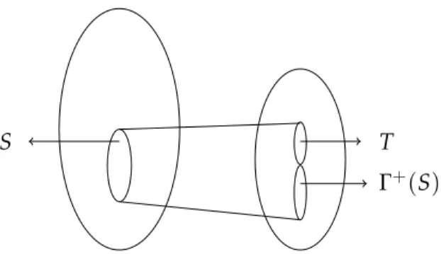
Proof. Consider the subgraph ofGinduced by S,Γ(S)and the edges that run between these sets. Partition the spaceΓ(S)intoΓ+(S)the set of unique neighbors and T :=Γ(S) \Γ+(S), the set of non-unique neighbors.
S
Γ+(S)
T
Figure 1.2 A representation of the set S⊆V and its neighborhood.
Note that we must have (
|Γ+(S)| + |T|)
=Γ(S) ≥γ|S|. (1.1)
On the other hand we can count the number of edges leaving both S andΓ(S)to conclude that
(|Γ+(S)| +2|T|) ≤∆V|S|. (1.2) Subtracting eq. (1.2) from twice eq. (1.1) yields the desired bound.
12
This lemma is at the heart of this analysis. It is important because it implies that the distance of the code is lower bounded.
Lemma 6. LetG be a (γ, δ)-expander such that γ ≥ ∆V/2. Then the distance of the associated codeC(G)is δn.
Proof. The distance of a code is the weight of the smallest codeword. Codewords by defi-nition will not be detected by any checks. Let e be an error such that its support is S ⊆V. Therefore at least one check will flag the pattern corresponding to|S|.
Expander graphs are interesting because they have a deceptively simple decoding algo-rithm called flip [24].
For the rest of the analysis we will require that γ ≥3∆V/4. Let x be the transmitted code-word and y be the received code-word. A check node c is said to be unsatisfied (or UNSAT) if the syndrome sc
sc:=
∑
v∈Γ(c)xv=1 (mod 2),
and satisfied (or SAT) otherwise. Equivalently, we shall say that the c-th syndrome bit is 1. The decoding algorithm flip is shown in algorithm1. The first few lines of the algorithm Algorithm 1 flip
Input: Received word yFn
2, syndrome s(e) ∈Fm2. Output: w ∈Fn
2
w :=y ▷Update w iteratively
F = ∅ ▷Flippable vertices
for u∈V do ▷Setup phase: update variable nodes
If u has more UNSAT than SAT neighbors, add it toF end for
while∃u∈ F do ▷Flip while flippable vertices exist
flip wu
UpdateΓ(u), and decide whether they are UNSAT UpdateΓ(Γ(u))and decide whether they are inF end while
Return w
are the setup phase. We shall iteratively maintain the word w until we arrive at the answer. If the algorithm terminates with no UNSAT checks, then we return w as the transmitted
codeword. The precomputation to obtain the syndrome is linear time. Indeed, there are m = O(n)check nodes and each has constant degree, so we can compute the syndrome vector s(e)in linear time.
The setup cost is linear time. There are n variable nodes and we can decide whether each node ought to be added toFin constant time as it only has a constant number of neighbors. Next, we study the main part of the algorithm within the while loop. Each step of the while loop is rather simple and takes constant time. How long does the while loop run? The number of unsatisfied checks is decreasing monotonically at each step. This immediately lets us prove the following claims.
Claim 7. LetG = (V∪C, E)be a bipartite graph with|V| =n and|C| =m be a(γ, δ)-expander graph. Let the total number of errors be ne, i.e. if y= x+e, then ne =wt(e). If we decode using flip, then
1. the decoding time is less than m.
2. the decoding time is less than∆Vne. Proof. We shall prove each claim in turn.
1. This is evident because the number of unsatisfied checks is monotonically decreasing. Since there are at most m checks, the algorithm will take time at most m.
2. If there are neerrors, then the number of unsatisfied checks is at most∆Vne. As above, we make use of the fact that the number of unsatisfied checks is monotonically de-creasing to arrive at the claim.
When does the flip algorithm return to the right codeword?
Claim 8. LetG = (V∪C, E)be a bipartite graph with|V| =n and|C| =m be a(γ, δ)-expander graph such that γ≥3∆V/4. Let the total number of errors be ne, i.e. if y=x+e, then ne=wt(e). If ne<δn/(∆V+1), then the decoding algorithm is guaranteed to succeed.
Proof. At each step of the algorithm, only a single bit is flipped. The weight of the error e is initially ne. Since the algorithm is guaranteed to conclude before∆Vnesteps, then the weight of the error can at most become(∆V+1)ne.
14
For the sake of contradiction, suppose that the algorithm has reached its last step. There are still uncorrected errors, but flip finds no more variable nodes to flip. In other words, there exist no variable nodes u such that they are connected to more UNSAT checks than SAT checks. However, since the weight of the error set is now at most(∆V+1)ne <δn, we can invoke the unique expander property. Therefore, if we let S denote the support of the error e, then it follows from lemma5that
|Γ+(S)| ≥ (2γ−∆V)|S| ≥ (∆V/2) |S|.
The second inequality follows from the assumption that γ ≥ 3∆V/4. Since the neighbor-hood of S contains at most∆V|S|elements, this means that there exists at least one variable node in S that has more unsatisfied neighbors than satisfied neighbors. Therefore this can-not be the penultimate step as there is at least one more variable node to flip.
This shows that the decoding algorithm terminates, and terminates on a codeword. How do we know that this is the right codeword? By assumption, the total number of errors on the word never exceeds (∆V+1)ne < δn. However, since the distance of the code is δn, we could not have mapped to the wrong codeword. In other words, if the algorithm had mapped us to some other word x′ ∈ C, then we would have h(x, x′) ≥ δn. This is impossible.
The flip algorithm takes as input a corrupted codeword y and returns the codeword x that was most likely transmitted. We have assumed that computing the syndrome in the setup phase of the algorithm could be done perfectly. When we consider the quantum equivalent, we shall see that we cannot directly peek at the quantum state, and our measurements might be imperfect. We will need to perform error correction in a fault-tolerant manner to ensure that we can overcome this. Although we will not cover the quantum proof because it is complicated, we offer a simpler, classical analogy.
In the face of syndrome errors, it will turn out that we cannot perform perfect error cor-rection. Rather, we will hope to merely reduce the number of failures on the code based on the number of errors on the syndromes. Buried within Spielman’s construction for effi-cient encoders [32] based on expander graphs is a proof that there exist good error-reduction codes(see lecture 18 of Prof. Sudan’s lectures). This construction merely uses flip again, showing that this simple algorithm suffices to reduce the error. In this generalized setting, flipwill accept as input both the corrupted codeword, as well as the corrupt syndrome and output the best possible word.
The construction begins with a n bit codeword x∈Fn
2. After transmission, we receive y := x+e, for some error e∈Fn
2. Let S= {v|yv ̸=xv} ⊆V be the set of indices corresponding to error locations. Similarly, let f ∈Fm
2 be the error on syndromes, i.e. the incorrect syndrome s′(y)is defined as s′(y) = s(y) + f for. Let E ⊆ C be the subset of check nodes whose syndromes are inferred incorrectly, i.e.
E= {c ⏐ ⏐ ⏐ fc =1 } .
In other words, these could correspond to either check nodes that are supposed to detect an error but do not, or check nodes that detect a phantom error.
We shall show the following result.
Lemma 9. Let G = (V∪C, E)be a (∆, 2∆)bi-regular (γ, δ)-expander. Suppose ∆ > 8 and γ> 78∆. Upon transmission of x, let the received word be y :=x+e and the syndrome be s′(y) = s(y) +f . If the total number of errors is nt≤δn/(∆+1), then flip(y, s′)outputs a word w such that the Hamming weight of w−x is upper bounded by 8|E|/∆.
Proof. Recall that the current state of the flip algorithm is labeled w ∈ Fn
2. Its syndromes corresponding to the c-th constraint is denoted sc(w)is said to be correct or SAT if
sc(w) =
∑
u∈Γ(c)wu (mod 2).
The idea here shall be that rather than iterate till all checks are SAT, we merely iterate till every message bit is adjacent to more SAT constraints than UNSAT.
Let nt <δn/(∆+1)be the total number of errors in both the codeword and the syndrome. The initial number of UNSAT constraints≤ ∆nt so the algorithm terminates in (at most) ∆ntiterations.
Over the course of the algorithm, each iteration flips at most one bit. Since the total number of iterations is upper bounded, the total number of message errors is upperbounded by (∆+1)nt <δn.
Note that Γ+(S) \E ⊆ UNSAT ⊆ Γ(S) ∪E. The first containment follows because the unique neighborhood of S will ideally detect the error pattern e. However, because the syndromes could have errors, it is onlyΓ+(S) \E that is guaranteed to be UNSAT. In other
16
The second containment follows because the set of UNSAT checks either correctly flags a real error in S or is detecting a phantom error and therefore in E.
This implies the following inequality: |UNSAT∩Γ(S)| ≥ (2γ−∆)|S| −2|E|. This follows because for two sets A, B, we have the identity|A∩B| = |A| + |B| − |A∪B|. Applying this above, we have
|UNSAT∩Γ(S)| = |UNSAT| + |Γ(S)| − |UNSAT∪Γ(S)| = |UNSAT| + |Γ(S)| − |Γ(S) ∪E| ≥ |Γ+(S) \E| − |E|
≥ (2γ−∆)|S| −2|E|.
This set is what we ultimately care about because it is the set that will determine if flip will terminate; if
|UNSAT∩Γ(S)| |S| >
∆ 2
then we are not done, as this means that at least one element of S has more than∆/2 un-satisfied neighbors. Equivalently, if the algorithm has stopped, then
2γ−∆−2|E| |S| ≤ ∆ 2 2|E| |S| ≥2γ− 3∆ 2 ≥ ∆ 4 |S| ≤ 8 ∆|E|.
The second chain of inequalities follows because γ≥7∆/8. Thus if ∆ >8, we are guaran-teed that the number of residual errors on the codeword is upper bounded.
1.3
Chapter summary
In this chapter, we reviewed the basic definitions of classical error correcting codes over the binary alphabet. We defined the central characteristics of a linear code – the number of bits n, the number of encoded bits k and the distance d. The distance was defined as the minimum number of bits that had to undergo an error for us to jump from one codeword in the codespace to another. We understood that codes could be defined using the parity check matrix. The parity check matrix checks that each codeword obeys certain linear constraints.
We proceeded to discuss an important class of classical codes called expander codes. We reviewed the definition of a bipartite graphG and how to associate a code to a graph. We noted that if the graphGis an expander graph, then many useful properties follow. Firstly, the distance of the associated code immediately follows from the expansion property. Fur-thermore, expansion also implies that the associated code possesses a simple decoding algorithm. This algorithm is called flip and simply flips bits to minimize the weight of the syndrome. We showed that this simple algorithm does indeed work if the graphGis a good expander. Finally we concluded by discussing how flip is fault tolerant. In other words, even if some of the syndrome bits are corrupted, flip succeeds in reducing the number of errors.
Chapter 2
Quantum Error Correction
How do we construct a quantum computer if circuit components are not perfect? As the size of the circuit increases, so does the likelihood of an error. The threshold theorem, one of the crown jewels of the theory of quantum computation, guarantees that we can in fact execute quantum computations of arbitrary length.
The key idea behind fault tolerance is to use quantum error correcting codes. Quantum error correcting codes serve as a buffer against noise – so long as too many errors do not accu-mulate, we can still recover the quantum information they encode. Error correcting codes thus permit us to simulate the circuit that we want to implement using another circuit that is more robust. This can then be repeated - we can encode the simulation in a simulation and reduce the error further until the desired level of robustness is achieved. The process is called concatenation and is the ingredient behind the first proofs of fault tolerance. At present, we believe that concatenation by itself will not suffice to build a quantum com-puter as the number of times we can reasonably concatenate a code is limited. Most efforts are focused on the surface code architecture, which in its simplest form does not involve concatenation. Another important difference is that the stabilizer generators of both surface codes and LDPC codes which we shall study later act on a constant-bounded number of qubits. These are much smaller than the number of errors t that the codes can correct. This contrasts with concatenated codes where each stabilizer acts onO(n) ≳ t qubits, so extra care must be taken when measuring a stabilizer in order not to create an uncorrectable er-ror in the process. Surface codes and LDPC codes thus have simpler syndrome extraction circuits. For a complete review of the fundamentals, see [33].
In this chapter we shall lay the foundation for what follows. We start by defining quantum error correcting codes and describing necessary and sufficient conditions for a quantum
code to be effective. Over the course of the chapter, we shall discuss guidelines for code construction. These guidelines, sometimes known as no-go results, are fundamental lim-its to quantum error correcting codes. We shall then overview techniques to manipulate encoded information and what we require to attain a universal gate set.
2.1
Quantum error correction
A quantum error correcting code is a way of storing quantum information redundantly. Broadly, a quantum error correcting codeCis a subspace of n-qubit states with some im-portant properties. Namely, these n qubits could be subject to some quantum noise channel E. A good code will allow us to recover the information stored inC by undoing the effect of the noise channelE.
At first glance, quantum error correction appears to be a wholly different enterprise than its classical counterpart. Quantum states could exist in coherent superpositions and mea-surement could potentially collapse the state. Further complicating the matter, errors on a qubit could be continuous rotations and therefore a continous set of errors against which to defend. However, the miracle of quantum error correction guarantees that it is possible to address these issues. We discuss each of them in turn.
Stabilizer group: A codeCis 2k-dimensional if it maps a k-qubit state|x⟩, where x∈ {0, 1}k is some k bit string, to an n-qubit state|x⟩for some n > k. Such a code space is spanned by vectors {|x⟩}x∈{0,1}k, where |x⟩ denotes the encoded version of the k qubit state |x⟩.
Each codeword|x⟩is itself the superposition of several computational basis states. We first address how to construct such states such that it facilitates measurement of the code space without collapsing the superposition. Codes shall be defined as the common eigenspace of a setS of commuting Pauli operators on n qubits.
C(S ) = {|ψ⟩ | |ψ⟩ ∈C2n
, S|ψ⟩ = |ψ⟩ ∀S∈ S }. (2.1) The setS is referred to as the stabilizer group and the generators of this group are called the stabilizer generators. Although the state ψ is in superposition, the stabilizer conditions stipulate that the code state can be measured without collapsing the state because it is an eigenstate of the stabilizer operator. In other words, the operators inS do not form a com-plete set of observables, so specifying their eigenvalue leaves some degenerate subspace where information can be stored. Equivalently, the code spaceCcan be specified by n−k independent stabilizer generators{Si}ni=−1k.
20
If the codewords ofCare corrupted due to some noise channelE, when can we recover the encoded quantum information? The fundamental theorem of quantum error correction due to Knill and Laflamme [34] states the conditions under which a quantum channel can be error-corrected by a specific codeC.
Theorem 10 (Knill-Laflamme). LetE be a noisy channel whose Kraus operators are{Ei}im=1, i.e. the action ofE on an n-qubit density matrix ρ is described as
E (ρ) =
∑
iEiρEi†.
The codeC is robust against the noise channelE if and only if
⟨x|Ei†Ej|y⟩ =cijδxy , (2.2)
where C=cij is some matrix.
The Knill-Laflamme condition helps us understand how we can correct against a very large class of (potentially continuous) errors. A key feature of eq. 2.2is that the constants cij do not depend on the codewords. A set of errors that obeys the Knill-Laflamme condition forms a linearly closed vector space, in the sense that if the set{Ei}obeys2.2, then so does the set{Fj}where each operator Fjis a linear combination of the operators{Ei}. Since the Pauli operators form an operator basis, any error Ei can be decomposed as a linear combi-nation of Pauli operators. We can therefore construct codes that correct a large number of Pauli errors, and by linearity this will extend to any error that is a linear combination of the correctable Pauli errors.
Of course, the quantum error correcting code is limited and cannot correct against all Pauli errors. One useful way of classifying correctable Pauli errors is by their weights, defined as the number of qubits on which the Pauli operator acts non-trivially. The minimum weight of an error E such that the Knill-Laflamme condition is violated represents the distance d of the codeC. It represents the minimum number of qubits that need to be affected to map one codeword to another. It follows that the Knill-Laflamme condition2.2 will hold for any set of errors of weight bounded by d−21. By linearity, 2.2 will also hold for any set of Kraus operators that are linear combinations of Pauli operators of weight bounded by d−21. Henceforth we focus on Pauli errors.
How to perform quantum error correction: Suppose a code state|ψ⟩ ∈ C, undergoes a Pauli error E,|ψ⟩ → |ψ′⟩ =E|ψ⟩. Error correction proceeds by measuring a set of stabilizer generators{Si}ni=−1k on the state|ψ
returns the outcome+1 by definition of the code spaceC. In the presence of errors however, we get Si ⏐ ⏐ψ′ ⟩ =SiE|ψ⟩ = ⎧ ⎪ ⎨ ⎪ ⎩ ESi|ψ⟩ = E|ψ⟩ = |ψ⟩′ if ESi = SiE −ESi|ψ⟩ = −E|ψ⟩ = − |ψ⟩′ if ESi = −SiE. ⎫ ⎪ ⎬ ⎪ ⎭ :=si(E) ⏐ ⏐ψ′⟩ . (2.3) These are the only two possibilities since Pauli operators either commute or anti-commute. In either case, the measurement outcome reveals the error syndrome bit si(E)which en-codes the commutation relation of the stabilizer generator Si and the error E that afflicted the system. The collection of all measurement outcomes(s1, s2, . . . sn−k)is called the error syndrome, and is used to determine the error E that occurred. The syndrome does not uniquely identify the error, so given an a priori distribution on the possible errors p(E), statistical inference is used to identify the most likely error. The algorithm that takes as input an error syndrome and returns an error guess is called a decoder. Note that multiple errors could have the same syndrome. We say that errors E and E′ are degenerate if for some stabilizer element S∈ S,
EE′ = S . (2.4)
Henceforth, such a code shall be called anJn, k, dK code. In other words, it uses n physi-cal qubits to encode k logiphysi-cal qubits and is capable of protecting the encoded information against(d−1)/2 errors.
Logical operators: The logical operatorsLof a stabilizer code map codewords of the code Cto other codewords of the codeC. Thus the logical operators map the codespace to itself, although their action on any individual codeword may be non-trivial. All the operators L ∈ L obey LS = SL, i.e. they commute with the codespace. Logical operators thus correspond to undetectable operators – if the code is afflicted by an error corresponding to L∈ L, we cannot detect it. Thus the distance d of the quantum error correcting codeCcan also be defined as the minimum weight of the logical operators inL. In what follows, this set may sometimes also be represented asN (S )or the normalizer of the stabilizer group. We focus on the logical X and Z operators of this space. Linear combinations and products of these operators generate the entire logical space, and clearly commute with the stabilizers. For simplicity, suppose the code only carried a single logical qubit, then there is only one pair of logical X and Z operators. Denoted by X and Z, their action on the codespace can
22
be described as follows. Let⏐⏐0⟩ denote the encoded logical|0⟩and ⏐
⏐1⟩ denote the encoded logical|1⟩. Then we have
X⏐⏐0 ⟩ = ⏐⏐1 ⟩ Z⏐⏐0 ⟩ = +⏐⏐0 ⟩ X⏐⏐1 ⟩ = ⏐⏐0 ⟩ Z⏐⏐1 ⟩ = −⏐ ⏐1⟩ .
These logical operators obey the anti-commutation relations XZ= −ZX.
In general, if the code carries k logical qubits, then the logical operators of the code can be described using 2k logical operators or equivalently, k pairs of Xiand Zi operators, where the subscript i indicates which logical qubit the operators correspond to. Each pair Xiand Ziobeys the corresponding anti-commutation relations.
2.2
CSS codes
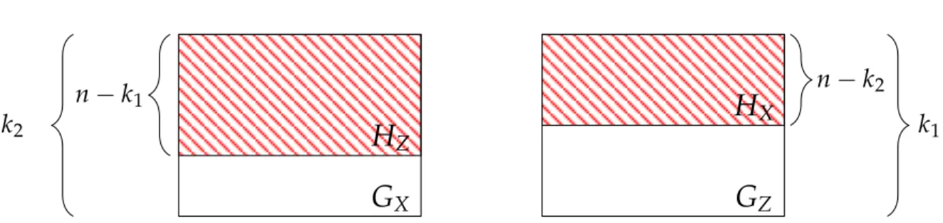
CSS codes are a template to form quantum codes from classical codes that obey certain constraints [35,36]. They are composed of two binary linear codesCZ = [n, k1, d1]andCX = [n, k2, d2]such thatC⊥Z ⊆ CX ⇔ CX⊥ ⊆ CZ. The spaceCX⊥andCZ⊥refer to the spaces of vectors that are orthogonal to all vectors inCX andCZ respectively. The resulting quantum code only contains stabilizers whose elements are all X or all Z. The constraints help guarantee that the resulting stabilizers commute. Suppose the parity check matrices of the codesCX andCZ are HX and HZ respectively. Let GX and GZ be the generator matrices for these spaces respectively.
To construct the code, we
1. map the ith row of HZ to Z stabilizer generator SZi by mapping 1’s to Z and 0’s to identity; and
2. map the jth row of HX to X stabilizer generator SXj by mapping 1’s to X and 0’s to identity.
This is depicted in fig. (2.1) where the red regions map to the stabilizer generators. For e, f ∈Fn
2, let X(e) = ⊗jXej and Z(f) = ⊗jZfj. Then Z(f)|w⟩ = (−1)⟨f ,w⟩|w⟩ X(e)|w⟩ = |w⊕e⟩ .
H
ZG
X n−
k1 k2H
XG
Z n−
k2 k1Figure 2.1 Quantum codes via the CSS construction. Two parity check matrices and codes
are shown. Red regions map to stabilizer generators.
The notation⟨f , w⟩ =∑i fiwi denotes the inner product between the strings f and w. With this correspondence between the space of vectors overFn2 and Pauli operators, it is easy to verify when two Pauli operators corresponding to X(e)and Z(f)commute. We have the condition[X(e), Z(f)] =0 if and only if⟨e, f⟩ =0 (mod 2).
The codewords correspond to cosets of CZ/CX⊥ and hence the code dimension is k := dim(CZ/C⊥
X )
=dim(CX/C⊥
Z).
The distance of a CSS code is then expressed as d=min{dX, dZ}where dX= min
e∈CZ\CX⊥
wt(e) dZ = min
f∈CX\C⊥Z
wt(f) .
This corresponds to the minimum weight of an undetectable error of X and Z type respec-tively.
Guidelines for code construction # 1: BPT bound
We have so far not discussed the geometry of our quantum error correcting code. It would be convenient if we could lay out our qubits in 2 dimensions, i.e. on a table top. Fur-thermore, it would be nice if we did not need to engineer too many connections – if each stabilizer was only connected to a handful of qubits. Finally, we might want to minimize ‘wire crossings’, i.e. such that all the qubits in the support of a stabilizer are right next to it. Unfortunately, such codes are highly restrictive.
The BPT bound, named after its discoverers Bravyi, Poulin and Terhal, states that the sur-face code captures everything we need to know about local codes (up to constant factors). They proved that anyJn, k, dK code in 2 dimensions defined by local stabilizer generators obeys the following bound:
24
Ignoring constants, this bound is saturated by letting d =O(√n). In the next chapter, we shall discuss one such code, called the surface code, which saturates this bound. If we want to get more bang for our buck, we might need to give up the constraint of locality.
2.3
Universal gate sets
A fault-tolerant computational scheme must be realized with a discrete set of universal gates. While physical gates can be tuned continuously, logical gates must belong to a dis-crete set to be correctable. Suppose for instance that the logical gate Rx(θ) := e−iθσx was permitted for any real value of θ in some fault-tolerant scheme. If some small error in the execution of the gate yielded the transformation Rx(θ+ϵ)instead, this would be indistin-guishable from an ideal circuit implementing a different logical gate, so this physical error would be promoted to an uncorrectable logical error.
Each gate in this discrete set can be corrected to any desired accuracy given an appropriate error-correcting code. If the gate set is universal, then any logical gate belonging to a con-tinuum can be approximated by a suitable sequence of gates from the discrete universal set. This is called gate synthesis.
The most common path to universality is formed of the CNOT, the Hadamard H and phase S := √σz = Rx(π4)which together generate the Clifford group. This is a finite maximal subgroup of the unitary group on n qubits. The Clifford group is the automorphism group of the Pauli group and its elements are completely characterized by their action on the generators of the Pauli group, i.e. on X and Z. For instance, the action of the Clifford group generators are
HXH† = Z CNOT(XI)CNOT†= XX HZH† = X CNOT(IX)CNOT† = IX
PXP† = iXZ CNOT(ZI)CNOT† = ZI PZP† = Z CNOT(IZ)CNOT† =ZZ
(2.5)
It is not universal and in fact Clifford circuits acting on computational basis state inputs and Pauli measurements can be efficiently simulated classically [37,38]. The fact that it is maximal means that adding any gate to this set produces a universal set of generators.
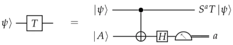
Common choices for this last gate are T := √S = Rz(π8), the Toffoli gate control-control-not, or the controlled-S gate. These all belong to the third level of the Clifford hierarchy, which means that for any Pauli operator P and any one of these third-level gate U, the combination UPU†is a Clifford gate. This will be important for state injection. In the case of T, efficient compilation algorithms are known [39] that take as input an arbitrary single-qubit gate U, and output a sequence of T and H of length 3 log(1
ϵ)that synthesize U to
accuracy ϵ.
2.4
Transversal gates
One of our main concerns when designing a fault-tolerant scheme is error propagation. If a qubit has suffered an error and is then involved in a two-qubit gate, then after the gate both qubits are potentially erroneous. If this occurred in a distance d = 3 code, then the
|φ⟩ |ϕ⟩
|ψ⟩
Figure 2.2 The state φ contains an error (indicated in red). After φ and ϕ interact via a
2-qubit gate, the resulting 2-2-qubit state ψ also potentially contains a 2-2-qubit error (indicated in red).
two-qubit gate has promoted a single-qubit correctable error to a two-qubit uncorrectable error.
One way to avoid this problem is to never couple two qubits from the same code block. Transversal gatesacting on single logical qubit are thus tensor products of single-qubit gates ⨂n
j=1Uj. Transversal gates involving logical qubits from two distinct code blocks are tensor products of two-qubit gates⨂n
k=1Uj1
k,j2k where the first qubit of a pair(j
1
k, j2k)belongs to the first code block and the second qubit belongs to the second code block, and each qubit appears in a single pair. While such a two-qubit transversal gate can transform a single-qubit error in a two-single-qubit error, these two errors will belong to different code blocks, so they will be correctable by the respective code on which they act.
Note that this definition of transversality was motivated by distance 3 codes which can correct at most one error. It ensures that all weight-one errors remain correctable, so if the physical error rate is ϵ, the effective logical error rate will beO(ϵ2). For a code with a larger minimum distance, we could demand that a generalized transversal gate increases the weight of an error by at most some constant a. Then, because the code can correct all
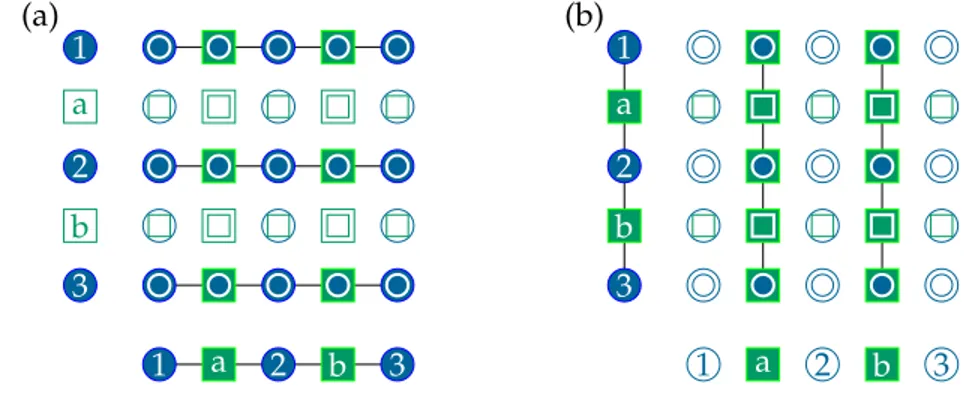
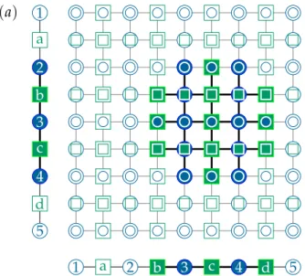
![Figure 3.1 (a) The surface code that results from a product of two [ 3, 1, 3 ] repetition codes.](https://thumb-eu.123doks.com/thumbv2/123doknet/4954358.122286/46.918.221.746.159.411/figure-surface-code-results-product-repetition-codes.webp)