A theoretical and experimental dissociation of two models of decision‐making

1

Université de Montréal

A theoretical and experimental

dissociation of two models of

decision-making

Matthew A. Carland

Département des neurosciences, Faculté de médecine

Mémoire présentée à la Faculté de médecine

en vue de l’obtention du grade de maîtrise

en sciences neurobiologique

August, 2014 © Matthew A. Carland, 2014

2

Abstract (French)

La prise de décision est un processus computationnel fondamental dans de nombreux aspects du comportement animal. Le modèle le plus souvent rencontré dans les études portant sur la prise de décision est appelé modèle de diffusion. Depuis longtemps, il explique une grande variété de données comportementales et neurophysiologiques dans ce domaine. Cependant, un autre modèle, le modèle d’urgence, explique tout aussi bien ces mêmes données et ce de façon parcimonieuse et davantage encrée sur la théorie. Dans ce travail, nous aborderons tout d’abord les origines et le développement du modèle de diffusion et nous verrons comment il a été établi en tant que cadre de travail pour l’interprétation de la plupart des données expérimentales liées à la prise de décision. Ce faisant, nous relèveront ses points forts afin de le comparer ensuite de manière objective et rigoureuse à des modèles alternatifs. Nous réexaminerons un nombre d’assomptions implicites et explicites faites par ce modèle et nous mettrons alors l’accent sur certains de ses défauts. Cette analyse servira de cadre à notre introduction et notre discussion du modèle d’urgence. Enfin, nous présenterons une expérience dont la méthodologie permet de dissocier les deux modèles, et dont les résultats illustrent les limites empiriques et théoriques du modèle de diffusion et démontrent en revanche clairement la validité du modèle d'urgence. Nous terminerons en discutant l'apport potentiel du modèle d'urgence pour l'étude de certaines pathologies cérébrales, en mettant l'accent sur de nouvelles perspectives de recherche.

Mots-clés: Prise de décision; modèle de diffusion; Modèle d’intégration; Modèle d’urgence; Discrimination perceptuelle; Compromis vitesse/précision; Mouvement aléatoire de points; Echantillonnage séquentiel; Test d’hypothèses; Temps de réponse; Comparaison de modèles; Neuro-économie; Taux de récompense

3

Abstract (English)

Decision-making is a computational process of fundamental importance to many aspects of animal behavior. The prevailing model in the experimental study of decision-making is the drift-diffusion model, which has a long history and accounts for a broad range of behavioral and neurophysiological data. However, an alternative model – called the urgency-gating model – has been offered which can account equally well for much of the same data in a more parsimonious and theoretically-sound manner. In what follows, we will first trace the origins and development of the DDM, as well as give a brief overview of the manner in which it has supplied an explanatory framework for a large number of behavioral and physiological studies in the domain of decision-making. In so doing, we will attempt to build a strong and clear case for its strengths so that it can be fairly and rigorously compared to potential alternative models. We will then re-examine a number of the implicit and explicit theoretical assumptions made by the drift-diffusion model, as well as highlight some of its empirical shortcomings. This analysis will serve as the contextual backdrop for our introduction and discussion of the urgency-gating model. Finally, we present a novel experiment, the methodological design of which uniquely affords a decisive empirical dissociation of the models, the results of which illustrate the empirical and theoretical shortcomings of the drift-diffusion model and instead offer clear support for the urgency-gating model. We finish by discussing the potential for the urgency gating model to shed light on a number of clinical disorders, highlighting a number of future directions for research.

Key words: Decision-making, Drift-diffusion model, Integration model, Urgency-gating model, Perceptual discriminations, Speed-accuracy trade-off, Random-dot motion, Sequential sampling, Hypothesis-testing, Response time, Model comparison, Neuroeconomics, Reward rate

4

TABLE OF CONTENTS

1. Introduction (p8)

1.1. The origins of decision models: the sequential sampling test (p8) 1.2. The “basic” drift-diffusion model (p11)

1.3. The “basic” DDM: a brief experimental history (p13) 1.4. The random-dot motion task (p13)

1.5. Model convergences (p15)

1.5.1. Noise (p16) 1.5.2. Biases (p16)

1.5.3. Non-decision delays (p17)

1.6. The ”pure” DDM (p17)

1.7. The ”pure” DDM: a brief experimental overview (p20) 1.8. Model divergences (p21)

2. Physiology (p22)

2.1. Neural evidence mechanisms (p23)

2.2. Neural evidence accumulation mechanisms (p24) 2.3. Neural threshold mechanisms (p27)

2.4. Summary: physiology (p29)

2.5. The current state of the sequential sampling framework (p30)

3. Revisiting the foundational assumptions of the DDM (p31)

3.1. Assumption #1: sequential sampling is required for simple perceptual judgements (p31) 3.2. Assumption #2: threshold settings are constant (p35)

3.3. Assumption #3: integration is required for noise compensation (p39) 3.4. Assumption #4: environments are generally stable (p40)

3.5. Assumption #5: sample commutativity (p41) 3.6. Summary (p43)

4. Introducing the urgency-gating model (p44)

4.2. Dynamical features of the UGM (p46) 4.3. Re-visiting physiology (p48)

4.3.1. Evidence signals (p48)

4.3.2. Accumulating and thresholding (p50)

4.3.3. Output variability in the UGM: intra- vs. inter-trial noise (p52)

4.4. Experimental differentiation of the models (p52)

5. Main experiment (p56)

5.1. Methods (p58) 5.2. Results (p63)

6. Discussion (p70)

6.1. Current evidence vs. total weight of evidence (p73) 6.2. The importance of filtering noisy input signals (p75) 6.3. Urgency, time pressure and reward rate (p77) 6.4. The wider significance of the UGM (p80)

6.4.1. Urgency signals and reward rate maximization: beyond RT (p80) 6.4.2. Potential physiological origins of the urgency signal (p84) 6.4.3. Urgency and delay discounting (p85)

6.4.4. Urgency in the aetiology of Parkinson’s disorder (p88)

5

LIST OF TABLES:

6

LIST OF FIGURES:

1: The “basic” drift-diffusion model (p11) 2: The “pure” drift-diffusion model (p18)

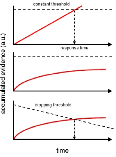
3: Evidence-accumulation and thresholding processes in area LIP (p28) 4: Constant vs. dropping thresholds (p38)

5: Sample commutativity in the DDM (p42)

6: The dynamic components of the urgency-gating model (p45) 7: Model turn-around times (p48)

8: The “tokens” task (p54)

9: The logic of the current experiment (p57) 10: VMD “bias” trial types (p61)

11: Reaction times for “no-pulse” trials in the blocked and interleaved conditions (p65) 12: Cumulative response time distributions for pulse- and no-pulse trials (p66)

7

LIST OF ABBREVIATED TERMS:

BA – Bias-against BF – Bias-for BG – Basal ganglia CMD – Constant-motion discrimination DDM – Drift-diffusion model DT – Decision time DU – Bias “down-up” FEF – Frontal eye fields LIP – Lateral intraparietal area PD – Parkinson’s disorder RDM – Random-dot motion RT – Response time

SC – Superior colliculus

TAFC – Two-alternative forced-choice task UGM – Urgency-gating model

UD – Bias “up-down”

8

Introduction

Writ large, “decision-making” can be abstractly described as an effortful, resource-intensive deliberation between competing options. By this formulation, decision-making is an essential feature of animal behavior and cognition, as animals must by necessity be able to acquire information about the environment and apply the information obtained therefrom to produce adaptive behaviors through which they can acquire the various resources they require for survival and propogation. To this end, animals are equipped with a brain that must accomplish this general task through sole reference to the information supplied to it by its sensory systems. As such, “adaptive behavior” necessarily entails the generation of- and deliberation amongst competing hypotheses both within and across multiple levels of the nervous system’s processes effectively mediating between sensory input, cognition, and motor output. Moreover, the brain must do so in real-time, and on the basis of a finite set of inherently probabilistic cues extracted from its diverse suite of sensory mechanisms. In this sense, then, “decision-making” is not only relevant to the complex cognitive processes connoted by its everyday meaning, but in fact comprises a fundamental computational process that is essential to the brain’s general operations (Gold & Shadlen, 2001; 2002; Bogacz et al., 2006; Yang & Shadlen, 2007).

The origins of decision models: the sequential sampling test

Importantly, the general process of employing probabilistic information to deliberate between multiple hypotheses is a problem that is not specific to animal cognition. In fact, the basic framework of hypothesis-testing can be formulated on purely mathematical grounds as a formal statistical problem (Gold & Shadlen, 2001; Bogacz, 2007). While the initial impetus for its mathematical formalization was provided by cryptographic efforts on the part of the Allies during World War II (for review see Gold & Shadlen, 2002), its core premises were subsequently adapted into a domain-general statistical process shortly following the end of the war efforts. The resulting domain-general formulation of hypothesis-testing involves three essential components (c.f. Good, 1979).

Firstly, the bearing of each “sample” on each of the hypotheses under consideration must be discretely quantified. In statistical terms, this amounts to defining a set of hypotheses, each of which implies a set of expectations about what kind of samples would be likely given that each hypothesis

9

were true. This allows for any given sample to be assigned a discrete probabilistic value according to how strongly it supports each of the hypotheses under consideration. Secondly, for any decision in which the informational content of a single sample is not sufficient to conclusively distinguish between the hypotheses (i.e. most decisions), a method is required by which individual samples can be combined to yield a quantitative measure of the total information presently available. This aspect of the hypothesis-testing procedure exploits a proven mathematical principle which states that multiple, statistically independent pieces of probabilistic information can be summated to produce a joint estimate of probability that is greater than any of its individual constituent parts (Pierce, 1878). This allows for multiple independent samples to yield a corresponding decrease in the uncertainty associated with two hypotheses for as long as more samples are acquired. Thirdly, a criterion must be set according to which either more samples are collected, or the decision is terminated in favor of one of the given hypotheses.

Together, these three features comprise the process of sequential analysis, in which the overall weight of evidence bearing on the hypotheses under consideration is updated given each new piece of evidence until sufficient information has been acquired to choose between one of two hypotheses at a desired level of confidence. Adapting this process from the domain of cryptography to a general statistical test resulted in the sequential sampling procedure (see Wald, 1945; Barnard, 1946; Wald, 1947; Wald & Wolfowitz, 1948; Lehmann, 1959) encompassing both a recursive sampling process as well as a “stopping rule,” or desired evidence criterion, which determines the point at which sampling is terminated and a corresponding hypothesis is chosen.

The addition of the “stopping rule” is crucial for two reasons. Firstly, it places a bound on the sampling procedure, which could otherwise be carried out indefinitely; this allows for a decision between hypotheses to be formally ended so that other, subsequent decisions can be made on the basis of the first decision’s outcome (Gold & Shadlen, 2000; 2002). Secondly, this stopping rule not only determines how many sampling iterations will be required, but also specifies the level of accuracy of the ensuing decision (Busemeyer & Townsend, 1993).

This abstract, domain-general process provides an appropriate conceptual framework for studying animal behavior, as animals must base their actions on a finite set of inferences about their environment, and accordingly must choose the actions that are the most likely to lead to the acquisition of their motivational needs (c.f. DeGroot, 1970). Thus, applying this conceptual framework

10

to animal behavior entails the following set of assumptions: (1) information is acquired in sequential fashion through the body’s extended range of sensory systems; (2) this information is interpreted with respect to a subset of potential reward-pursuit behaviors that are currently afforded by the environment, thereby providing “evidence” for- or against certain “hypotheses” representing specific courses of action; (3) this evidence is “accumulated” over the course of the deliberation process, resulting in a gradual decrease in the uncertainty associated with the potential actions under consideration which is proportionate to the total amount of accumulated evidence; (4) the deliberation ends when uncertainty has been reduced to a certain level corresponding to the desired accuracy of the decision, at which point the action entailed by the winning “hypothesis” is initiated. This conceptual framework enabled the formulation of empirical tests following the insight that the “length” of the sequential sampling procedure – as represented by the number of sampling iterations entailed by any particular instantiation of the test – is analogous to the amount of time used by an animal to make a decision on the basis of a given set of observations (Stone, 1960). Re-casting this abstract framework for hypothesis-testing into an explicitly temporal domain has two major consequences. Firstly, the quality of the evidence obtained will have a direct impact on how quickly the decision is made, such that more informative samples will cause the uncertainty to decrease at a faster rate (Ratcliff, 1978). Secondly, the stringency of the decision criterion will also determine how long a decision takes, with more accurate decisions requiring more sampling time (Busemeyer & Townsend, 1993; Gold & Shadlen, 2002; Bogacz et al., 2006).

Consequently, a trade-off necessarily arises between the speed of a decision and its accuracy (Swensson, 1972; Pachella, 1974; Wickelgren, 1977; Bogacz et al., 2006; Balci et al., 2011), and in this respect the sequential sampling framework conforms to a long-known principle governing action-based decisions (Woodworth, 1899; Garret, 1922; Hick, 1952). How this trade-off is managed is of no small consequence to real-world decision-makers, who must balance between maximizing both their total opportunities for reward (i.e. the total number of decisions they can make within a given period of time, as determined by the speed of their decisions) and their likelihood of successfully obtaining a reward from a given decision (i.e. the success or accuracy of their decisions; see Cisek et al., 2009; Balci et al., 2011; Thura et al., 2012). Thus, for any given environment, decision criteria that are less stringent will lead to faster but less accurate decisions, and criteria that are more stringent will lead

11

to slower but more accurate decisions (Ratcliff, 1978; Gold & Shadlen, 2002; Bogacz, 2007; Balci et al., 2012).

The basic drift-diffusion model

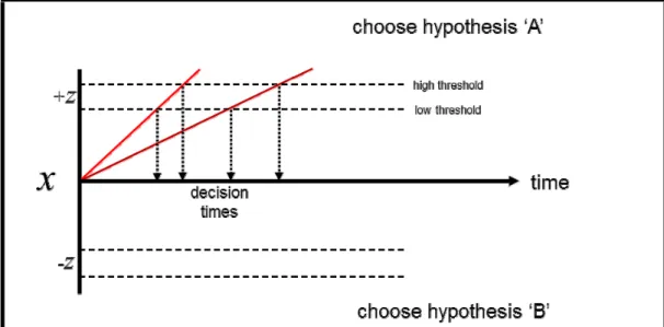
The sequential sampling framework served as the foundation for a number of early decision models which treat decisions as an iterative process during which a single variable tracks the cumulative evidence for favoring one hypothesis relative to another as increasing numbers of samples are obtained; sampling is continued until the total amount of accumulated information meets the decision criterion, at which point the decision process is terminated and a corresponding action is undertaken (Ratcliff, 1978; Mazurek et al., 2003). Any such model can be said to constitute a discrete analogue of a sequential sampling procedure, and therefore posits a set of broad mutual dependencies between evidence quality, decision criteria, and the amount of time required for a decision to be made. The basic foundational model is depicted in schematic form in figure 1.

Figure 1: the “basic” drift-diffusion model. Light and dark red traces represent the

model’s response to stronger and weaker evidence, respectively (captured by the

drift-rate variable A in formula #1). The point at which each trace crosses the

threshold determines the timing of the response. Response time (RT) is thus jointly determined by both the evidence strength (A) and the value of the threshold (±z).

12

We will refer to the basic, schematic model illustrated in figure 1 as the basic drift-diffusion model (DDM), which can be defined by the following equation:

dx = Adt, x(0) = 0

(1)

As illustrated in figure 1, the process encompassed by equation #1 above can be schematically conceptualized as unfolding within a two-dimensional decision space. One of its dimensions is symmetrically delineated by the decision bounds (±z). These are analogous to the “stopping rule” in the sequential sampling test, and therefore represent the quantity of evidence required to terminate the decision process in favor of each of the two hypotheses under consideration (NB: while these “decision bounds” are given different names among various models, for the sake of terminological consistency we will hereafter refer to these as the decision thresholds). A decision formally begins with the initialization of a decision variable (dx) at a starting value of zero; this value – together with the symmetry of the decision bounds (±z) – reflects the assumption that both hypotheses are considered to be equally likely prior to the acquisition of any samples. The variable (x) denotes the difference between the evidence supporting the two opposing hypotheses at any given time (t). The decision variable dx is continuously updated as the decision process unfolds, and thus at any given time reflects the sum of all previously-accumulated evidence. Adt represents the increase in x during

dt: A therefore determines the drift rate of the decision variable over the course of the decision

process, and is analogous to the “quality” of the evidence used as input to the model (i.e. higher values of A amount to a faster rate of change in the decision variable dx, and therefore lead to faster decisions).

As the evidence grows in favor of one hypothesis, support for the opposing choice necessarily dimishes; the evolution of dx over time as more samples are acquired subsequently resembles a

diffusion process between the two bounds (the feature after which the model was eventually named;

see Ratcliff, 1978). A decision is made when the decision variable dx crosses either of the two thresholds ±z, and the time of crossing is the response time (RT). Speed–accuracy trade-offs arise in the model as a direct result of the threshold setting (±z), such that lower thresholds lead to faster- but less accurate decisions, whereas higher thresholds lead to slower- but more accurate decisions (Domenech & Dreher, 2010; Forstmann et al., 2010; Balci et al., 2011).

13 The “basic” DDM: a brief experimental history

The mutual dependencies among decision factors entailed by the sequential sampling framework provided a set of tractable experimental hypotheses regarding the effects of evidence quality on the timing of decisions, and thereby laid the groundwork for experimental investigations of decision-making behavior. Empirical testing of the basic DDM model typically involved presenting subjects with a binary decision between two mutually-exclusive options, resulting in a class of task paradigms which came to be known as two-alternative forced-choice (TAFC) tasks (Schall, 2001; Gold & Shadlen, 2002). While many TAFC tasks were developed across a wide range of psychological domains (see Green & Luce, 1973; Ratcliff, 1978; Gronlund & Ratcliff, 1989; Ratcliff & McKoon, 1989; 1995; Wagenmakers et

al., 2004; 2008), the nascent field of decision-making research ultimately converged on a number of

psychophysical tasks, a handful of which today constitute the dominant experimental paradigms for most decision-making research. Early psychophysical tasks included judgments of dot separation, luminance discriminations, numerosity judgement, and binary color discriminations (Ratcliff & Rouder, 1998; Ratcliff et al., 1999; Rouder, 2000); however, the random-dot motion (RDM) task has come to be one of the prevailing and most ubiquitous experimental tasks for investigating the foundations of the decision-making process. In large part this is because it allows for the precise experimental definition of each relevant task factor, thereby facilitating the empirical quantification of changes in choice behavior engendered by manipulations to any of the discrete decision variables (Parker & Newsome, 1998).

The random-dot motion task

The RDM task is named after its stimulus, which consists of an image sequence showing a group of moving dots. Upon each frame, a fraction of these dots are selected to be re-drawn along a vector corresponding to the location of one of several peripheral targets, and the rest of the dots are moved randomly (Britten et al., 1993). The nature of this stimulus allows for the precise quantification and manipulation of “evidence strength,” expressable as the percentage of dots comprising its coherent motion signal. The relevance of this motion signal to the choice targets is easily learned, as the direction of the coherent motion signal corresponds to the location of the peripheral targets which are used by the subject to report the decision outcome. The strength of this signal then corresponds to “evidence strength” in a straightforward way, as a greater degree of motion coherence is more easily detectable, and is thereby analogous to higher-quality “samples” (Drugowitsch et al., 2012).

14

The RDM task yields two behavioral measures; the overt time of response corresponds to the duration of the cognitive procees underlying the decision, and accuracy rates (in the form of percentage of correct responses) allow for the inference of the value of the decision variable at the time of decision.

In its original formulation, the RDM task typically employed coherent motion signals that were

constant, in that they maintained a single value throughout the entire duration of a given trial (Britten et al., 1993; Cisek et al., 2009); however, some subsequent studies have adapted this task to

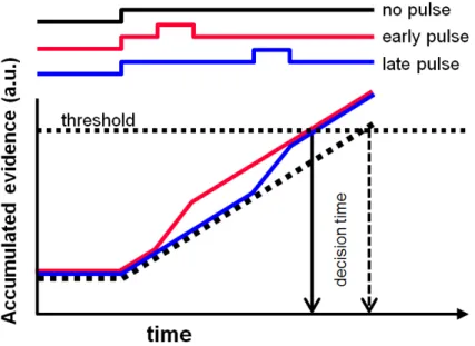
incorporate a changing-evidence signal, in which the evidence strength is varied throughout the course of a trial (e.g. Huk & Shadlen, 2005; Kiani et al., 2008; Tsetsos et al., 2012). This is most commonly accomplished via the insertion of motion “pulses” within trials, during which the motion signal is altered for a brief period (typically 100-200ms; see Roitman & Shadlen, 2002; Huk & Shadlen, 2005; Wong et al., 2007; Kiani et al., 2008; Thura et al., 2012). Despite the fact that these pulses are not consciously perceivable, they nonetheless have been shown to yield detectable effects on subject behavior; adding motion pulses tends to engender faster response times, whereas subtracting motion prolongs the decision duration, consistent with the predictions of the basic DDM (Roitman & Shadlen, 2002; Tsetsos et al., 2012). However, while motion pulses have been the most common way of varying the evidence presented in the RDM task over time, other studies have used more dynamic forms of changing evidence (Cisek et al., 2009; Thura et al., 2012; 2014), and we will discuss these in greater detail in later sections.

Importantly, because all the relevant task variables in the RDM can be precisely quantified, it allows for experimenters to manipulate individual variables and explain their impact on the subject’s overall behavior from within the basic framework of the DDM. For example, adjusting the motion coherence present in any given trial is equivalent to setting the drift-rate parameter (A; see equation #1); thus, the DDM predicts that for a given evidence strength, accuracy ought to improve as viewing time is increased, because the decision variable will be able to accumulate a greater number of samples, therefore resulting in more accurate decisions. Conversely, for any given amount of stimulus viewing time, the drift rate (A) will determine the final value of the decision variable, with greater values of (A) corresponding to more accurate decisions. Thus, accuracy in fixed-viewing-duration tasks ought to be directly related to the evidence strength (i.e. motion coherence) on any given trial (see figure 1).

15

Indeed, decision-making research is replete with behavioral studies that have extensively corroborated these predictions not only through the use of the RDM task (e.g. Britten et al., 1992; 1993; Gold & Shadlen, 2000; Roitman & Shadlen, 2002; Mazurek et al., 2003; Ditterich et al., 2003; 2006b; Ratcliff & Smith, 2004; Huk & Shadlen, 2005; Palmer, Huk & Shadlen, 2005; Bogacz et al., 2006; Kiani et al., 2008; Drugowitsch et al., 2012) but also through a variety of other psychophysical and cognitive tasks (Stone, 1960; Laming, 1968; Green & Luce, 1973; Pachella, 1974; Link, 1975; Link & Heath, 1975; Wickelgren, 1977; Ratcliff, 1978; Luce, 1986; Gronlund & Ratcliff, 1989; Ratcliff & McKoon, 1989; Link, 1992; Carpenter & Williams, 1995; Hanes & Schall, 1996; Schall & Thompson, 1999; Reddi et al., 2003; Wagenmakers et al., 2004; 2008; Smith & McKenzie, 2011). Thus, the early success of the DDM arose from its ability to attribute particular changes in overt measures of behavioral performance to manipulations of specific model parameters, and this ability has come to represent the benchmark test for all decision models in general. This overarching framework for evaluating decision models been referred to as the principle of “selective influence” (see Rae, Heathcote et al., 2014), by which a model is considered successful to the extent that it can capture an overt difference in behavior induced by a given experimental manipulation with a simple parametric change.

Ultimately, the employment of the basic DDM framework enabled the earliest decision-making researchers to amass a large body of behavioral data that subsequently guided the development of increasingly sophisticated sequential-sampling based models. Consequently, the first several decades of decision-making research led to a number of mechanistic additions to the basic DDM, several of which became universally adopted. We will discuss three of these in particular in what follows.

Model convergences

Originally, the mechanistic simplicity of the “basic” model outlined above consistenty led to major inaccuracies in its predictions. Chief among these was its fundamental inability to reproduce the variable distributions of response times commonly obtained in real animal subjects, who do not respond in exactly the same way to otherwise identical trials (Busemeyer & Townsend, 1993). Furthermore, the model was also unable to account for how erroneous decisions could arise – a major shortcoming, especially in light of the fact that subjects rarely attain perfect accuracy even for very easy discriminations (McElree & Dosher, 1989; Ratcliff, 1978; Reed, 1973; Usher & McClelland, 2001). Such problems were not unique to the basic DDM family of models, but also plagued a number

16

of other early models, such as signal-detection-theory models (Green & Swets, 1966) and stage theory

models (Sternberg, 1969; for historical overviews see Townsend & Ashby, 1983 and Busemeyer &

Townsend, 1993); however, the DDM ultimately superceded these other model classes when it fixed these shortcomings with the addition of a small number of features, to which we now turn.

Noise

The first – and most important – revision to the basic DDM was the addition of random variability in the model’s mechanisms. This addition was motivated not only by ubiquitous findings of variable RT distributions in behavioral data (Pachella, 1974; Link & Heath, 1975; Wickelgren, 1977; Ratcliff, 1978; Ratcliff & Smith, 2004), but was further grounded in the assumption that subjects cannot perfectly calibrate their decision-making parameters to exactly the same state across otherwise identical trials (see Ratcliff & Smith, 2004). This assumption was also plausible on biological grounds, as inherent variability arising at multiple levels of the nervous system would manifest as minor variations in decision behavior to otherwise identical stimulus input (Gold & Shadlen, 2001; 2002; Mazurek et al., 2003).

While noise could be implemented in any number of ways, the most common solution took the form of adding random variability to each “sample” fed to the model (Bogacz et al., 2006; Balci et al., 2011), thereby producing minor variations in the decision variable’s threshold-crossing time (Busemeyer & Townsend, 1993; Ratcliff, 2001). Adding noise to the models in this way allowed them to generate orderly, regular distributions of response times (Ratcliff & Smith, 2004; Bogacz et al., 2006). In fact, adding this single mechanism to previous, more rudimentary models was often enough to fix them considerably (Ratcliff & Smith, 2004; Bogacz et al., 2006; Bogacz, 2007). Ultimately, the role of noise in modeling the decision process is so crucial that its inclusion or omission is by itself often enough to make the difference between a model successfully accounting for data and its complete failure to do so (c.f. Van Zandt & Ratcliff, 1995).

Biases

However, there remained a few consistent discrepancies that were not fully redressed by the addition of sampling noise alone. For example, it was consistently observed that response-time distributions for correct trials differed significantly from those for error trials (Laming, 1968; Ratcliff, 1985; Ratcliff

17

variable’s initial value, such that noise-driven fluctuations during evidence accumulation were more likely to result in erroneous responses when the decision variable’s initial value had been biased slightly in favor of the incorrect choice (Laming, 1968; Luce, 1986; Ratcliff, 1978; 1981; Vickers, 1988). However, while the earliest implementations of these starting-point biases were implemented purely as noise, later models made such variability a freely-varying parameter in the model whereby the decision process could incorporate various “intentional,” “systematic” biases in choice behavior that were sometimes observed in decision tasks (Smith, 1994; Van Zandt & Ratcliff, 1995; Ratcliff & Rouder, 1998; Ratcliff, Van Zandt, & McKoon, 1999). This allowed for the basic DDM to effectively incorporate a broader range of latent cognitive processes related to choice preference, expected value, differences in choice costs, etc. (see Busemeyer & Townsend, 1993), thereby extending the ecological validity of the schematic model.

Non-decision delays

Lastly, given the prominence of response times as a core empirical measure for most tasks, obtaining accurate measurements thereof was obviously of crucial methodological importance (c.f. Pachella, 1974). While most early empirical studies employed cued-response tasks (Stone, 1960; Laming, 1968; Link, 1975; Link & Heath, 1975; Ratcliff, 1978; Kiani et al., 2008) in which the decision time was dictated by the experimenter, the increasingly widespread use of free-response paradigms (Luce, 1986; Link, 1992; Carpenter and Williams, 1995; Roitman and Shadlen, 2002; Mazurek et al.., 2003; Ratcliff and Smith, 2004; Lo and Wang, 2006) led to refinements in empirical measures of decision time. Because subjects in free-response conditions could respond while the stimulus was still being presented, the overt measure of their response time would necessarily be contaminated by a number of covert sensory- and motor-related delays – which if uncompensated for would lead to over-estimations of the subjects’ “true” decision time (Pachella, 1974; Ratcliff & Tuerlinckx, 2002). Most tasks began to include obligatory estimations of subjects’ mean reaction time, which could subsequently be subtracted from their overt response times to yield a more veridical estimate of the duration of the underlying decision process (Luce, 1986; Balci et al., 2012).

The “pure” DDM

Subsequent to the solution of these modeling discrepancies, the “basic” DDM was updated to include the above three features, and consequently became the dominant decision model on which most

18

models are based. Having thus reviewed the motivations behind these fairly ubiquitous model additions, we now re-introduce the relatively simple version of the DDM defined previously with a richer, more elaborate version which has served as the de facto standard model to the present day.

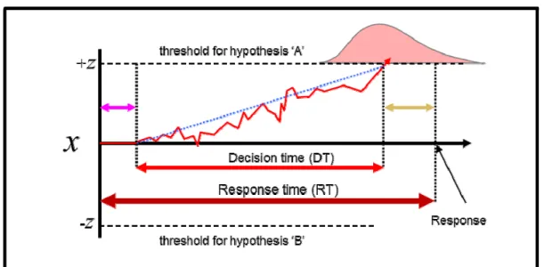
Figure 2: the “pure” drift-diffusion model. The pink and yellow arrows

indicate sensory and motor delays (respectively) – which when subtracted from the overt response time (RT) yield an estimation of the “true” decision time (DT) spent accumulating evidence to threshold. As before, the average time taken for the decision process is determined both by the threshold setting (±z) and the average quality of the evidence (A, dotted blue line); however, for any given decision, small noise-driven offsets in the value of the evidence input will cause slight variations in the overall decision time, yielding a stereotypical distribution of response times (light red distribution, top). Offsets in the initial value of x (variable b in formula #2; not pictured above) provide a further means of changing response time by making one hypothesis more or less likely at the onset of the decision process.

19

Adding the features discussed above to the “basic” DDM defined by formula #1 yields the following first-order stochastic differential equation, which we will subsequently refer to as the “pure” DDM:

dx = Adt + σdW, x(t

) = b

(2)

As in the previous formula, the decision variable dx effectively implements a random walk between two symmetric decision thresholds, and the rate at which this decision variable “drifts” between them is determined by the magnitude of the evidence values drawn from the distribution A. However, in this model, each sample drawn from A is assumed to contain an unknown amount of noise, supplied in the above formula by the term dW, which represents white noise drawn from a Gaussian distribution with a mean of 0 and a variance of σ2dt (c.f. Balci et al., 2012). Furthermore, the

decision variable is assigned an intial value of b; this value can be freely adjusted to implement an initial bias in the decision process such that a positive value of b makes the positive threshold a priori more likely to be chosen by decreasing the distance between the starting point of evidence accumulation and the positive threshold (and vice versa for negative values). Lastly, while the decision

time (DT) in this formulation is identified with the time of first crossing of the decision variable across

one of the decision bounds (±z), the model yields an additional time measure – the response time (RT) – which is the sum of the decision time and the sum of non-decision-related latencies t0 reflecting the

contribution of various sensory encoding- and motor execution delays to the observed time of a subject’s response. Subtracting an estimate of these non-decision delays from the overt response times observed during experimention thus yields a more precise estimate of the underlying cognitive decision process (Balci et al., 2012).

The specific implementation of noise in this “pure” DDM results in each sample having a small, random offset (either positive or negative) from its “true” value. However, while this adds a degree of uncertainty to the value of each sample, the assumption of a normal distribution of noise with a mean of 0 means that adding multiple noisy samples together over time will tend to cause the noise component to cancel out, leaving a veridical estimate of the underlying signal. Because the DDM effectively adds multiple independent samples together over time, this very process of successive sample integration provides the model with an intrinsic means for counteracting the distorting influence of noise (Ratcliff & Rouder, 1998; Bogacz et al., 2006; Bogacz, 2007; Balci et al., 2011). Consequently, in this version of the DDM “…the relative contribution of noise to the decision variable

20

diminishes as the number of samples accumulated increases, thereby decreasing the likelihood for noise-driven errors to arise as decision thresholds are increased, and thereby reinforcing the relationship between decision threshold and accuracy already latent in the basic DDM” (Bogacz et al., 2006). This cancellation of noise via the addition – or integration – of multiple samples over time has explicitly served as a further theoretical argument in favor of the pure DDM, because the coupling of this implementation of noise with the integrative process of sequential sample summation endows the model with all the benefits of intra-trial variability in the stochastic decision process while simultaneously providing a concrete mechanism by which much of its potential distorting effects can be canceled out (Bogacz, 2007). The mechanisms of this model therefore not only effectively provide some protection against noise, but further allow the model to account for speed-accuracy trade-offs better than the noiseless, “basic” version of the DDM (Laming, 1968; Ratcliff et al., 1999; Mazurek et

al., 2003; Bogacz et al., 2006; Bogacz, 2007). The “pure” DDM: a brief experimental overview

The “pure” DDM has been successfully applied to all manner of tasks across a number of distinct psychological domains, wherein it successfully predicts and explains the influence of various task manipulations involving evidence strength and viewing time on overall decision behavior (Stone, 1960; Laming, 1968; Vickers, 1970; Link, 1975; Link & Health, 1975; Ratcliff, 1978; Luce, 1986; Hanes & Schall, 1996; Schall & Thompson, 1999; Ratcliff & Rouder, 2000; Schall, 2001; Shadlen & Newsome, 2001; Gold & Shadlen, 2002; Ratcliff, Thapar, & McKoon, 2003; Ratcliff, Gomez, & McKoon, 2004; Smith & Ratcliff, 2004). In other words, it accurately describes and replicates discrete changes in decision behavior by uniting the various latent cognitive factors into a singular mechanistic framework that explains and predicts their interactions on overall decision behavior. Moreover, its ability to do so conforms to the previously-stated principle of “selective influence,” by which a model is evaluated according to the extent that it can successfully describe empirically meaningful changes in behavior in terms of manipulations of a small number of the model’s relevant parameters.

Due to its foundations in the sequential sampling framework it also describes speed-accuracy trade-offs, which are intrinsic to the model and arise as a straightforward consequence of the mechanisms it encompasses. Furthermore, the DDM’s mathematical tractability supplies it with a further advantage, in that a mathematically optimal set of parameters for the DDM can be objectively derived for any given task setting, which will produce the greatest average reward rate for any task,

21

provided that the distribution of trial difficulties are specified (Ratcliff & Smith, 2004; Bogacz et al., 2006; Bogacz, 2007; Simen et al., 2009). This aspect of the DDM has allowed for the empirical demonstration and quantification of optimality in natural animal behavior. Such demonstrations are typically founded on the assumption that in most experimental settings as well as in real-world environments, animals are motivated to achieve the highest possible reward rate over time (as opposed to optimizing their decision process on an individual-trial basis; see Cisek et al., 2009; Balci et

al., 2011; Thura et al., 2012). Thus, sequential sampling models – and, by extension, the “pure” DDM

derived therefrom – can therefore provide discrete mathematical solutions to speed-accuracy trade-off-related phenomena that are a typical feature of cognitive tasks in general (Swensson, 1972; Wickelgren, 1977; Luce, 1986; for overview see Balci et al., 2011).

Model divergences

In presenting the “pure” DDM above, it bears mentioning that the sequential sampling framework from which this model was developed has ultimately given rise to a large number of derivative models, among which there are almost as many specific mechanistic differences as there are individual models. This diverse plurality of models can in part be attributed to the fact that the sequential sampling framework was originally developed from outside the context of any particular domain of application, therefore leaving many of its finer implementational details unspecified; in other words, its basic mathematical formulation does not greatly constrain the particular ways in which its essential dynamics may be implemented. While the “pure” DDM – or integration model – shown above is currently the prevailing, dominant model in the field, it is nonetheless only the most prominent member within a diverse family of models which all have their theoretical roots in the sequential sampling framework.

Nonetheless, even where individual sequential-sampling-based models differ in subtle ways, in general they tend to agree on substantive questions of interpretation (Donkin, Brown, Heathcote & Wagenmakers, 2011). In fact, most models can be mathematically incorporated into the DDM, even when they differ significantly in the dynamics they afford. This has been demonstrated mathematically in a number of large-scale model-comparison studies (see Ratcliff & Smith, 2004; Bogacz et al., 2006; Bogacz, 2007). Accordingly, the “pure” DDM can be considered a fair representative for the many closely-related models that have their common roots in the sequential sampling framework (c.f. Cisek et al., 2009).

22

The ultimate test for any model is how well it can constrain and explain the actual physiological implementation of the decision process as it occurs in the brain (Platt & Glimcher, 1999; Gold & Shadlen, 2002; Purcell et al., 2010; Turner et al., 2013). Where models make identical or similar predictions, but differ in their mechanistic implementations, the most sensible recourse for deciding between them is to assess their individual mechanisms in terms of their biological plausibility.

In this light, the convergence of many models on a limited range of essential features provides a set of concrete and empirically well-established proscriptive hypotheses regarding what sorts of decision-making mechanisms may exist in the brain (Ratcliff & McKoon, 1995; Gold & Shadlen, 2002; Churchland et al., 2008). Specifically, these ought to include functionally-analogous neural implementations of several major decision factors including 1) sensory evidence signals; 2) the encoding of accumulated integrated evidence, and 3) decision thresholds. Finding evidence for similar mechanistic processes in the brain would therefore constitute further proof that sequential-sampling models are the appropriate framework for studying natural decision-making behavior. In what follows, we briefly outline the body of physiological evidence that has emerged as a result of the DDM’s considerable history of empirical success.

Physiology

The convergence of multiple models on the limited range of essential features encapsulated in the extended DDM model presented above can be considered to provide a set of relatively concrete and empirically-corroborated tentative hypotheses regarding what sorts of decision-making mechanisms may exist in the brain (Gold & Shadlen, 2002; Bogacz, 2007). However, given the mathematical complexity of many of the operations involved in the models, it is unlikely that real-world decision-makers are actually computing precise probability estimates, integrating samples perfectly, etc. (Cisek

et al., 2009; Rae, Heathcote et al., 2014). Instead, the models are taken as representing the “essential

dynamic properties” (c.f. Tuckwell, 1988) of the decision process, and the specific mathematical computations implied by such models are otherwise assumed to be realized in approximated form by the underlying neural system (Busemeyer & Townsend, 1993). Therefore, the mathematical descriptions and procedures suggested by the DDM and related sequential-sampling-based models are taken only as a general framework whose dynamic properties and individual mechanisms neural

23

computations can plausibly be fitted to approximate, and any neurobiological theory of decision-making will have to be constrained by the types of computational mechanisms that are actually achievable by biological neural networks. Accordingly, the search for neural implementations ought to entail looking for plausible, neurally-realizable approximations of the essential dynamic properties exhibited in abstract form by the models themselves (c.f. Tuckwell, 1988; Busemeyer & Townsend, 1993).

Neural evidence mechanisms

The extensive use of psychophysically-oriented experimental paradigms in decision-making research meant that the well-characterized anatomical localization of much of the brain’s sensory-processing hierarchies could be exploited to constrain potential areas of interest, given the provisional assumption that the evidence signals relevant to a given decision ought to be at least in part supplied by sensory areas whose functional profiles correspond to the discriminations entailed by a given task. In fact, the RDM task was itself originally developed from a simple noisy motion-detection task meant to elucidate the functional properties of extrastriate visual cortical area V5/MT (Morgan & Ward, 1980; Seigel & Anderson, 1986), and was subsequently taken up by Newsome & Paré (1988) who adapted it to its current form for the purposes of providing direct proof for its role in supplying the evidence during perceptual decisions in the RDM task. To date, a wide array of subsequent single-cell recording studies have now yielded substantial evidence that the firing rates of direction-selective cells in area MT during a random-dot motion task are linearly correlated with the relative strength of the coherent motion in the stimulus, and that this activity can be “read-out” to predict the accuracy of a subject’s decision (Newsome et al., 1989; Britten et al., 1992; Britten et al., 1993; Britten et al., 1996; Shadlen et al., 1996). Moreover, its role in the decision process has been further demonstrated by both focal chemical inactivation (Newsome & Paré, 1988) and electrical microstimulation (Salzman

et al., 1990; 1992; Salzman & Newsome, 1994; Ditterich et al., 2003) of MT cells, such that

manipulations of neuronal activity in this region can effectively delay or hasten the ensuing behavioral response. The ability for manipulations of MT activity to influence the decision process suggests a directly causal role for area MT in supplying evidence for decisions relying on motion-based stimulus cues such as the RDM, in a manner that is mechanistically analogous to the evidence signal posited by the DDM (specifically, its activity essentially appears to encode the drift-rate variable (A) from formula #2 above; see Ratcliff & Smith, 2004; Bogacz et al., 2006; Balci et al., 2011).

24

Furthermore, the general role of supplying evidence for a perceptual discrimination appears to generalize beyond the specific functional contributions of area MT to a RDM task. A number of other studies have located similar evidence-coding activity during other tasks, supplied by different sensory processing areas whose respective functional profiles correspond to the nature of the perceptual discrimination being tested; these have included cortical areas related to somatosensory (Salinas et

al., 2000; Romo & Salinas, 2003; Houweling & Brecht, 2008; Hernández et al., 2010), auditory (Sally &

Kelly, 1988; Kaiser et al., 2007; Yang et al., 2008; Jaramillo & Zador, 2011; Bizley et al., 2013; Znamenskiy & Zador, 2013), olfactory (Uchida & Mainen, 2003; Uchida et al., 2006) and non-motion-related visual processing (Heekeren et al., 2004; 2008; Yang & Maunsell, 2004; Kosai et al., 2014). Thus, taken together, this extensive body of studies has demonstrated a neural implementation of evidence signals derived from sensory input that provide a quantitatively-graded signal compatible with the putative role of evidence signals in the decision process as posited by the DDM.

Neural evidence accumulation mechanisms

The evidence-coding signals provided by the cortical regions identified above appear to represent the current evidence, but do not perform the accumulative functions otherwise crucial to the DDM’s essential dynamics; thus, such signals had to be found elsewhere. As before, the search for evidence-accumulating functions was guided by a number of provisional hypotheses afforded by the experimental history of the DDM. In the case of most of the experimental tasks employed in decision-making studies, subjects are already aware of the mapping between the relevant stimulus dimensions and the specific motor responses used to report the decision outcome (Gold & Shadlen, 2000; Yang & Shadlen, 2007). For example, the “motion evidence” for a RDM task is not evidence about “motion direction” in an abstract sense, but rather is evidence for the specific behavioral response used to report the decision and thereby obtain a reward (Platt & Glimcher, 1999; Gold & Shadlen, 2000; 2002; Yang & Shadlen, 2007). Consequently, this insight motivated the adoption of the provisional physiological hypothesis that evidence accumulation may take place in high-level motor command structures responsible for issuing the behavioral response required by a given task (Platt & Glimcher, 1999; Gold & Shadlen, 2000).

This prediction has been borne out by a wide range of studies which have yielded extensive evidence for such mechanisms among a diverse range of cortical and extracortical sites. In the superior colliculus (SC), for example, a number of experimental studies featuring tasks in which a subject’s

25

decision is reported with a saccade have revealed that the relative activity of collicular neurons strongly covaries with both the probability and magnitude of a reward associated with the cell’s spatial target over the course of the decision period (Basso & Wurtz, 1998; see Ratcliff, Cherian & Seagreaves, 2003 for overview). Other studies have revealed a number of suggestive correlations between the build-up of activity in individual collicular neurons and both the likelihood (Dorris & Munoz, 1998; Dorris et al., 2000) as well as the latency (Basso & Wurtz, 1998; Everling et al., 1999; Dorris et al., 2000) of an ensuing saccade into the response field of the recorded cells. Finally, the baseline activity levels of these collicular cell populations at the time of a decision’s onset appear to reflect a predisposition to choose a target in the corresponding space of the visual field (Horwitz & Newsome, 1999; 2001), consistent with the biasing mechanisms featured in the “pure” DDM defined in equation #2. Collectively, these studies provide compelling support for the hypothesis that the superior colliculus serves as a physiological site for bridging the accumulation of decision evidence with the principal behavioral output of that decision (i.e. a saccade), which is itself consistent with the well-established functional role of the SC in coordinating and executing oculomotor behaviors (Basso & Wurtz, 1998; Dorris & Munoz, 1998; Everling et al., 1999).

Physiological assays of other cortical regions have furnished further support for this overarching neural hypothesis. For example, the well-characterized functional role of the frontal eye fields (FEF) in coordinating and initiating eye movements motivated a series of studies using the RDM task to establish a direct correspondence between neural activity in FEF cells and the development of an ongoing decision. These studies ultimately showed that direction-selective cells in this region appear to implement the accumulation of information during a RDM task, with neural activity building up as a function of both motion strength and viewing time (Gold & Shadlen, 2000; Ding & Gold, 2012), consistent with the dynamics of the decision variable in a DDM model (for an analogous example of such neural activity recordings from Roitman & Shadlen’s (2002) study of area LIP see figure 3, below).

Finally, similar findings have also been obtained in the lateral intraparietal area (LIP), another cortical area with an empirically well-substantiated role in the spatial coordination of oculomotor behavior (see Platt & Glimcher, 1999; Roitman & Shadlen, 2002). Here, once again, a number of physiological assays have revealed the effective neural implementation of a developing decision via single-cell recordings in this area (Gnadt & Anderson, 1988; Hanes & Schall, 1996; Platt & Glimcher, 1997; Colby

26

& Goldberg, 1999; Platt & Glimcher, 1999; Shadlen & Newsome, 2001; Roitman & Shadlen, 2002; Leon & Shadlen, 2003; Dorris & Glimcher, 2004; Sugrue, Corrado & Newsome, 2004; Hanks, Ditterich & Shadlen, 2006; Ipata et al., 2006; Yang & Shadlen, 2007). Further consistent with corresponding studies of other brain areas mentioned previously, area LIP also exhibits quantitatively-graded decision-related buildup of activity whose rate of growth is commensurate with the strength of the evidence both for tasks in which the evidence input is continuous (as in an RDM task; see see Roitman & Shadlen, 2002; Ratcliff, Cherian & Segraves, 2003; Smith & Ratcliff, 2004; Gold & Shadlen, 2007; Kiani, Hanks & Shadlen, 2008) as well as when the evidence arrives in discrete units over time (Yang & Shadlen, 2007). Additionally, further single-unit recording studies of cellular activity in LIP have led to the suggestion that the encoding of accumulated evidence appears to take place in probabilistic units of log-likelihood, which is further consonant with the general framework of sequential sampling at large (see Wald, 1947; Gold & Shadlen, 2002; Yang & Shadlen, 2007). In other words, the qualitatively-graded activity of LIP cells appears to reflect the brain’s ability to extract and accumulate probabilistic evidence from sensory information over time (Yang & Shadlen, 2007).

Finally, physiological recording in area LIP has established that the temporal profile of decision-related activity in this region is consistent with the hypothesis that LIP is in direct receipt of input from a number of extrastriatal visual areas known to play a role in the types of psychophysical discriminations commonly featured in decision tasks (see Roitman & Shadlen, 2002; Shadlen & Newsome, 2001; Hanks, Ditterich & Shadlen, 2006; Huk & Shadlen, 2005; Yang & Shadlen, 2007; and references therein). For example, Kiani, Hanks & Shadlen (2008) used an RDM task to show that the total latency between the time of stimulus onset and LIP responses falls within a window of ~210-260ms, which suggests a delay between LIP and its putative motion-related evidence input from MT that is only approximately ~100ms (Britten et al.., 1996; Bair et al.., 2002; Roitman and Shadlen, 2002; Osborne et al.., 2004; Huk and Shadlen, 2005). Conversely, this suite of temporal relationships between LIP and the cortical sensory areas which presumably provide it with its fundamental input is further consonant with anatomical studies that suggest that sensory areas including MT/V5 and V4 are anatomically well-poised to supply feedforward input to areas encoding the total accumulated evidence, such as FEF and LIP. This has been demonstrated in explicit anatomical terms by a number of physiological studies documenting reciprocal cortico-cortical connections across a range of visual sensory and parietally-situated motor control centers, including those between LIP and MT & V4 (Blatt, Anderson & Stoner, 1990) as well as between MT and both LIP and FEF (Ungerleider &

27

Desimone, 1986). Thus, LIP in particular appears to be a central hub in decision-making activity, which together with a diverse set of cortical sensory-processing areas appear to constitute a widely-distributed network for decision-making.

However, it must be noted that LIP’s role in decision-making is not wholly accounted for; for instance, it has been shown that LIP activity can exhibit responses to a number of extended factors which can not themselves be definitively attributed to evidence-related processing, such as target value (Platt & Glimcher, 1999; Sugrue et al., 2004), reward expectation (Sugrue, Corrado & Newsome, 2004; Dorris & Glimcher, 2004), or even the mere passage of time (Ditterich, 2006a; Beck et al., 2008; Churchland

et al., 2008; Hanks et al., 2011; Standage et al.., 2011). Ultimately, however, such findings are not

themselves inconsistent with the general role of area LIP in evidence accumulation presented here; in fact, these influences may all be indicative of a more general role for LIP in coordinating behavior in response to a wide variety of task-relevant variables (Rao, 2010). However, we will return to the topic of non-evidence-dependent activity in LIP in later sections, and will for now merely note that its wider functional profile has not been entirely determined.

Neural threshold mechanisms

Lastly, while empirical evidence has been presented for the neurobiological implementation of evidence estimation and accumulation in a number of brain regions, the implementation of a decision threshold remains to be established. The DDM posits that the threshold is set at a constant level, and that the crossing of this threshold by the decision variable determines the timing of the ensuing response. This therefore suggests that demonstrating the existence of analogous neural decision thresholds would require measuring neuronal activity while a decision was completed, and analysing this activity to see whether decision times could be predicted on the basis of the decision variable having reached a common activity level across multiple trials. Importantly, however, most behavioral tasks studied in laboratory experiments have been fixed-duration studies (Rieke et al., 1997; Parker & Newsome, 1998); thus, when the stimulus viewing duration is controlled by the experimenter, the true decision time is covert, thereby prohibiting a precise estimation of the subjects’ actual decision time (Britten et al. 1993; Shadlen & Newsome 2001; Parker et al. 2002; DeAngelis & Newsome 2004; Krug 2004; Krug et al. 2004; Uka & DeAngelis 2004). Therefore, the use of free-response tasks was empirically necessary to identify neural mechanisms analogous to the threshold mechanisms suggested by the DDM (see Kiani, Hanks & Shadlen, 2008).

28

Figure 3: Evidence-accumulation and thresholding processes in area LIP.

Responses of LIP neurons during a random dot-motion discrimination task, from Roitman & Shadlen (2002). Left: alignment of neural activity on stimulus onset reveals that the rate of neural activity build-up diverges as a function of the evidence strength. Right: alignment of neural activity on saccade onset reveals that the oculomotor response is initiated when LIP activity reaches a fixed common level of activity corresponding to the threshold in the DDM.

To date, the clearest demonstration of direct neural mechanisms of thresholding comes from a physiological study of area LIP by Roitman & Shadlen (2002), who recorded single-cell activity rates over the course of a decision in a RDM task. The free-response nature of this task enabled the researchers to directly investigate what happens in these neural populations at the time when accumulation stops and an overt behavioral response is initiated. They found that aligning neural activity on the estimated time of decision onset revealed that the transition from gathering sensory evidence to acting on this information appeared to occur at the moment at which accumulative

29

neural activity in area LIP reached a fixed, absolute level that was consistent across trials (see figure 3). Additionally, the threshold at which the build-up of neuronal activity terminated and triggered an outcome-reporting movement was identical for both correct and incorrect trials, therefore indicating that these LIP neurons do not reflect the objective direction of the stimulus motion, but rather indicate the subjects’ belief about the decision evidence (Roitman & Shadlen, 2002; Yang & Shadlen, 2007).

A series of subsequent studies have also corroborated the finding of absolute neural activity thresholds during decision-making, the crossing of which predicts both the ultimate choice and the timing of the subject’s behavioral report (Ratcliff, Cherian & Segraves, 2003; Mazurek et al., 2003; Kiani et al., 2008; Ding & Gold, 2012). Taken together, these studies have collectively shown that LIP activity can be consistently seen to rise toward a common firing-rate threshold that is independent of a specific trial’s motion coherence as well as the ensuing decision time. The fact that the final firing rate value was common across all conditions suggests that the threshold is constant, with variations in decision timing being due to corresponding differences in the underlying factors governing the rate at which this activity builds up, at least part of which would be evidence-related (Roitman & Shadlen, 2002; Mazurek et al., 2003; Kiani et al., 2008).

Summary: physiology

In general, the studies reviewed in the foregoing would appear to confirm the neural implementation of evidence signals, evidence accumulation, and thresholding mechanisms as posited by the DDM. More recently, the anatomical and functional details of the emerging neurobiological scheme has led to the suggestion that decision processes take place on a level of neural organization that effectively links sensory, cognitive and motor processes within a common domain, thereby facilitating the rapid conversion of sensory information into behavior in real-time, consistent with the ecological demands of real-world behavior (Gold & Shadlen, 2000; Cisek, 2007).

Ultimately, the emergent functionality of these many individual neural mechanisms strongly conform to the mechanistic predictions made by the DDM, and therefore have typically been interpreted as evidence for a more-or-less direct (if approximate) neurobiological implementation of the decision process as outlined in mathematical abstraction by the sequential sampling framework at large (Gold & Shadlen, 2002). More broadly, these findings appear to substantiate the notion that animal

30

behavior is broadly analogous to hypothesis-testing, for which evidence is accumulated over time and summated to provide an informed (but still inherently probabilistic) estimate of the state of the world, and therefore by extension the best course of action that the environment currently affords (Gold & Shadlen, 2002; Bogacz et al., 2006).

The current state of the sequential sampling framework

As we noted earlier, a number of crucial mechanistic additions were made to the “basic” DDM (equation #1) in order for it to successfully capture a number of common features in behavioral data. While these mechanisms were universally adopted (and led to the highly successful “pure” DDM; equation #2), many divergent and increasingly-complex models continued to be developed over time. Problematically, however, the progressive diversification and mechanistic embellishment of the ever-growing family of sequential-sampling-based models has been accompanied by a corresponding tendency for the ensuing models to become capable of mutual “mimicry,” by which any sufficiently complex model can match the output of any other by mere virtue of the fact that its mechanistic complexity ensures that a set of parameters can almost always be found which will reproduce the output of a competing model (see Bogacz, 2007; Tsetsos et al., 2011; 2012; Rae, Heathcote et al., 2014). Thus, as models become more complex they necessarily become more flexible in their ability to fit data – but it cannot therefore be concluded that such a model necessarily represents the best or most parsimonious explanatory framework for the observed phenomena. Instead, an alternative evaluative framework is required to resolve disputes between models without recourse to the models’ abilities to reproduce the predictions of another.

On this point, several recent studies have presented data that resists explanation by the DDM (Usher & McClelland, 2001; Cisek et al., 2009; Thura et al., 2012; Tsetsos et al., 2012). While adherents of the DDM have sucessfully addressed a few of these challenges with parametric modifications (see Ratcliff & Smith, 2004; Bogacz et al., 2006; Bogacz, 2007; Kiani et al., 2008), many of these empirical challenges remain outstanding. Despite these suggestive demonstrations of the DDM’s potential shortcomings, however, these studies have generally not considerably undermined the DDM’s status as the prevailing model. In fact, the DDM has been continued to be acknowledged as the de facto model even by modelers with personal allegiances to alternative models (see Usher & McClelleand, 2001; Wang, 2002; Wong & Wang, 2008; Cisek et al., 2009; Balci et al., 2011; Thura et al., 2012; Tsetsos et al., 2012).

31

Thus, the persistence of the DDM in the face of such empirical challenges serves to highlight a broader potential problem with the reigning methodology of decision research; that is, it could be argued (and has been: see Rae, Heathcote et al., 2014) that the ability of the DDM to replicate the output of models that otherwise differ substantially in their dynamics may have unintentionally precluded the search for alternative (and potentially more parsimonious) models by obscuring the theoretical utility of such alternatives behind a strategy of continued parametric revisions. Instead, to prevent over-commitment to a singular, increasingly-mechanistically-embellished model, the core assumptions on which models are built must be continually questioned to clear the ground for potential alternatives. Accordingly, we proceed along these lines by revisiting and reconsidering some of the core assumptions underlying the DDM in its current form to see if there may be just cause to resume the search for models that deviate substantially from the essential framework of the DDM which, because of the DDM’s status as the default paradigm, would not otherwise be searched for.

Revisiting the foundational assumptions of the DDM

Assumption #1: sequential sampling is required for simple perceptual judgments

The core functionality of the DDM rests on the assumption that a single sample is rarely sufficient to make an informed decision; thus, it relies on the integration of multiple samples over time to exploit the intrinsic relationship by which decision accuracy can be increased by accumulating additional samples, and this mechanism is directly responsible for the model’s output of a decision variable that grows over time. Taking the logic of the DDM to its natural conclusion, then, would lead to the straightforward prediction that decision accuracy ought to increase monotonically for as long as sampling is continued. That is, even a particularly difficult perceptual discrimination, if given enough time, ought to eventually reach near-perfect levels of accuracy. Problematically, however, this prediction is not borne out in the extensive body of data on perceptual discrimination tasks. Instead, it has been consistently observed that success rates tend to asymptote after a certain amount of viewing time, even when additional sampling time is provided (Wickelgren, 1977; Shadlen & Newsome, 2001; Usher & McClelland, 2001; Roitman & Shadlen, 2002; Huk & Shadlen, 2005; Kiani et

al., 2008). For example, when Roitman & Shadlen (2002) controlled their subjects’ viewing time

32

difficult trials in which additional viewing time should have been of significant benefit to the subject. While this appears to occur in all trials regardless of difficulty, the amount of time it takes for accuracy to stabilize at a consistent final level appears to be dependent on the strength of the evidence in a given trial; very strong evidence leads to near-instant saturation of accuracy rates, whereas relatively difficult discriminations appear to lead to asymptoting accuracty rates after between 800ms (Roitman & Shadlen, 2002; Kiani, Hanks & Shadlen, 2008) and 1000ms (Usher & McClelland, 2001; Tsetsos et al., 2012).

However, the above studies all employed RDM tasks, which therefore leave open the possibility that this phenomenon could be task-specific. However, a number of studies using different behavioral tasks have also yielded data suggesting that decisions tend to be made on the basis of information arriving in a window of time which is often substantially shorter than the full length of the decision process itself (Cook & Maunsell, 2002; Ludwig et al., 2005; Luna et al., 2005; Ghose, 2006; Uchida et

al., 2006; Yang et al., 2008; Kuruppath et al., 2014; but see also Burr & Santoro, 2001). Together,

these studies would appear to argue against a traditional conceptualization of integration as a decision-making mechanism, and instead seem to suggest that there is some limit to the utility of extended sampling that instead motivates subjects to base decisions on only a subset of the total information presented to them. In other words, the apparent mechanisms purportedly implementing evidence integration may actually be serving a different purpose.

Two resolutions to these observations have been previously proposed. On one hand, adherents to the DDM family of models have proposed that the decision process is cognitively taxing, and that subjects therefore simply allot a limited amount of time to the formulation of a decision. Consequently, they argue that the saturation of accuracy rates can be explained by an early truncation of the decision process such that subjects are satisfied with a given level of performance for a given difficulty; accordingly, they claim that subjects integrate samples until they reach the desired threshold, and simply ignore all further information (Kiani et al., 2008).

If this were true, then it would follow that manipulations of evidence within a trial should only be effective in changing subjects’ behavior if these changes occur early in the trial, i.e. while the animal is still integrating evidence. In other words, decision-makers ought to exhibit primacy biases, such that early decision information should matter more than later information. Indeed, such primacy biases have been shown by several studies (Huk & Shadlen, 2005; Kiani et al., 2008). However, other studies