This is an accepted manuscript of an article published by Elsevier in Transportation Research Part D on June 6 2014, available at http://dx.doi.org/10.1016/j.trd.2014.05.001 This manuscript version is made available under de CC-BY-NC-ND 4.0
license http://creativecommons.org/licenses/by-nc-nd/4.0/ Please cite as:
Carrier, M., Apparicio, P., Séguin, A.-M., & Crouse, D. (2014). The application of three methods to measure the statistical association between different social groups and the
concentration of air pollutants in Montreal: A case of environmental equity. Transportation Research Part D: Transport and Environment, 30, 38-52. doi:10.1016/j.trd.2014.05.001
Title: The application of three methods to measure the statistical association between
different social groups and the concentration of air pollutants in Montreal: a case of
environmental equity
Journal: Transportation Research Part D
Authors and affiliations
Mathieu Carrier, PhD candidate* - Corresponding author
385 rue Sherbrooke Est, Montréal (Québec), Canada
H2X 1E3
[email protected]
(514) 499-8249
Philippe Apparicio, PhD
385 rue Sherbrooke Est, Montréal (Québec), H2X 1E3
[email protected]
Anne-Marie Séguin, PhD
385 rue Sherbrooke Est, Montréal (Québec), H2X 1E3
[email protected]
Dan Crouse, PhD
805 rue Sherbrooke Ouest, Montréal (Québec), H3A 0B9
McGill University
[email protected]
Référence complète de l’article:
Carrier, M., Apparicio, P., Séguin, A-M. et Crouse, D. (2014) The application of three methods to measure the statistical association between different social groups and the concentration of air pollutants in Montreal: A case of environmental equity, Transportation Research Part D, 30, 38-52.
Abstract
Analyzing the spatial dispersion of pollutants has led researchers to develop measures in order to determine whether certain population groups are disproportionately exposed to these hazards. A proxy of the distance from major roads, mathematical modelling, and exposure as established by pollutant measurement are three of the main techniques developed to determine environmental inequity with regard to a particular group in the broader population. A number of the studies performed have concluded that the low-income population and, to a lesser extent, visible minorities tend to reside in the most polluted areas. The main objective of this article is to compare the results obtained from three techniques for analyzing the spatial concentration of pollutant emissions on the Island of Montreal. The second objective is to determine whether groups vulnerable to air pollutants—namely, individuals under 15 years old and the elderly—and those who tend to be located in the most polluted areas—i.e., visible minorities and the low-income population—are affected by environmental inequities associated with air pollution. The results obtained from the three techniques for evaluating environmental equity firstly show that there are differences between these techniques. Secondly, they show that the groups selected based on age are not affected by environmental inequities. Finally, they indicate that the low-income population and, to a lesser extent, visible minorities in Montreal more frequently live near major roads and in areas with higher pollutant concentrations.
Keywords: environmental equity, air pollution, transportation, pollutant indicators, GIS Highlights
Three techniques are used to measure air pollution in residential areas
We compare the results obtained from the three techniques
We determine whether the selected groups tend to live in polluted areas
The environmental equity assessment varies according to the three techniques
1. Introduction
In urban areas, vehicular exhaust along transportation networks is the primary source of ambient air pollution, including nitrogen oxides (NOx) and, to a lesser degree, carbon monoxide (CO) and particulate matter (PM). Both short- and long-term exposure to urban air pollution can be harmful to human health (Brunekreef and Holgate, 2002). Moreover, living within 200 metres of a major road is considered a potential risk to cardiovascular health (Brugge et al., 2007; Rioux et al., 2010), and for the development of asthma (Jerrett et al., 2008; McConnell et al., 2006) and lung development deficits among children (Gauderman et al., 2007). Previous studies have argued that the combination of socioeconomic inequalities and exposure to air pollutants contributes to physiological vulnerability among members of low-income households (Brulle and Pellow, 2006; Kohlhuber et al., 2006; O'Neill, 2007). Other studies have noted that the health impacts of pollution are greater among children and the elderly. Indeed, children are more vulnerable to the effects of exposure to air pollutants because their organs and nervous systems are not fully developed (Bolte et al., 2009) and they breathe in more air per unit of body mass (Landrigan et al., 2004). In the case of the elderly, this vulnerability to air pollution is heightened due to their reduced immunity to disease particularly as a result of the aging of their vital organs. In addition, because children and the elderly are less mobile, they are more confined to their residential environments (Day, 2010; Greenberg, 1993; Philipps et al., 2005). If these environments offer poor conditions, these groups will be more affected than those in other age categories.
1.1 Environmental equity and air quality
The literature on environmental equity focuses especially on the distribution of nuisances and resources, which, because of the unequal spatial distribution of different social groups, leads to an increased exposure to risks or to less access to beneficial elements for certain populations. The current view associated with environmental equity can be defined as follows: “Environmental justice policies seek to create environmental equity: the concept that all people should bear a proportionate share of environmental pollution and health risk and enjoy equal access to environmental amenities” (Harner et al., 2002). Studies performed in various countries have shown that low-income households tend to be exposed to substantially higher levels of ambient pollution than more affluent households, even though they have fewer vehicles (Brainard et al., 2002; Chakraborty, 2009; Kingham et al., 2007; Morello-Frosch et al., 2001). Results from environmental equity research related to ethnic minorities vary between countries and by context (Ringquist, 1997). For example, in the United States, a
number of studies (e.g., (2009; 2002; 2001) have shown positive associations between the presence of ethnic minorities and concentrations of air pollutants. In Canada, however, with the exception of Latin Americans in Hamilton, Buzzelli and Jerrett (2004, 2007) found no relationship between the proportions of ethnic minorities and concentrations of ambient pollution in the cities of Hamilton and Toronto. In a previous study in Montreal, Crouse et al. (2009b) found only weak positive associations between exposure to nitrogen dioxide (NO2) and the percentage of visible minorities at the census tract level. Despite their physiological vulnerability to exposure to air pollution, the categories of children and the elderly have been addressed less often in environmental equity studies. Chaix et al. (2006) have nonetheless reported that children under 15 years old from low-income households in Malmö, Sweden, were in general exposed to higher NO2 levels than children of the same age with higher socioeconomic status. As for the population over 65 years of age, Brainard et al. (2002), Mitchell and Dorling (2003), and Chakraborty (2009) found no environmental inequity experienced by children in relation to air pollution exposure in Birmingham (United Kingdom) and Tampa Bay (United States). Collins et al. (2011), on their part, examined disparities linked to risks of cancer from pollutant emissions in El Paso, Texas, and concluded that Hispanics aged 65 and older were more likely to develop various health problems compared with the white population of the same age. So, studies on children and the elderly have arrived at different conclusions in different geographical contexts.
1.2 Local measurements of air pollution
In the past 20 years or so, various methodological approaches have been proposed for evaluating pollutant exposure among vulnerable groups by using spatial analysis methods. First among these is proximity to sources that generate air pollutants, an approach that has often involved defining “buffer zones” ranging from 0 to 300 metres (m) around major roads (Amram et al., 2011; Bae et al., 2007; Cesaroni et al., 2010; Chakraborty, 2006; Chakraborty et al., 1999; Green et al., 2004; Gunier et al., 2003; Houston et al., 2006; Jacobson et al., 2005) or creating density indices based on road network hierarchy (Houston et al., 2004). To evaluate environmental equity, logistic regression is often modelled with a binary dependent variable indicating whether a census tract or city block is located at least n metres from a section of highway (200 m, for example), and with independent variables describing the proportions of targeted groups (e.g., ethnic minorities) within buffers of various radii. This approach has come under criticism, however, as the use of a binary variable may conceal substantial variations in exposure in terms of concentration. Two different city blocks may, for instance, be located within 200 m of a highway: one at 10 m, and the other at 190 m.
Furthermore, some blocks may be located at the same distance from the highway (50 m, for example), but be surrounded by very different overall lengths of highway sections within a 200-metre radius. To solve this problem, some authors (Apparicio et al., 2008; Gunier et al., 2003; Houston et al., 2004; Rioux et al., 2010) recommend creating density indices, based on either traffic volume or roadway hierarchy.
The second most frequently used technique is mathematical modelling. This approach consists in estimating pollutant concentrations based on data relating to traffic volumes as well as meteorological information such as temperature, wind force, and wind direction (Kingham and Dorset, 2011). The advantage of this technique is that it enables the generation of a spatial dispersion map for air pollutants on a large scale: for example, a given city. However, some authors, such as Kingham and Dorset (2011), point out that the accuracy of these models can vary significantly depending on the data and parameters integrated into the model, and particularly according to meteorological factors. A few studies have used a mathematical dispersion model to study environmental equity. Their general aim is to measure statistical associations between pollutant levels such as PM10 (Kingham et al., 2007; Pearce and Kingham, 2007), NO2 (Brainard et al., 2002; Chaix et al., 2006; Kruize et al., 2007; Mitchell and Dorling, 2003), or several pollutants (Briggs et al., 2008) obtained through modelling, on the one hand, and several variables related to deprivation and to proportions of ethnic minorities or children, on the other. To this end, several statistical methods have been used, including regression models, and nonparametric tests. The final technique consists in constructing spatial statistical or geostatistical models to predict pollutant concentrations for an entire territory based on locations where pollutants are measured using samplers (most often for NO2) over a given period. NO2 is the pollutant most often used to measure pollution concentrations generated by road transportation, since it has high co-locational association with other types of pollutants such as PM and CO (Beckerman et al., 2008; Wheeler et al., 2008). Once the pollution measurements are collected at n points across a study area, several different kinds of models can be used to generate a surface map, including geostatistical interpolation methods such as kriging (Buzzelli and Jerrett, 2004; Jerrett et al., 2001), or land-use regression (Croland-use et al., 2009a; Jerrett et al., 2007). The advantage of this spatial modelling, as Kingham and Dorset (2011) have noted, is that it allows pollutants to be measured at a much finer scale, and at relatively low cost. However, the technique has no longitudinal scope since it is based on pollution data measured at a specific time and under conditions specific to the time of sampling.
2. Research questions and objectives
A few authors have highlighted the fact that the spatial association between certain groups and an environmental phenomenon may be different if a measure is taken directly versus provided through a proxy (Kingham and Dorset, 2011; Maantay et al., 2010; Walker, 2010). Bowen (2002) also showed that the results could be different depending on the scale and the method used. Most et al. (2004) analyzed the impacts of spatial scale and population assignment choices in an excessive noise case in the United States. Their findings reported that the results vary according to the methodological choices (Most et al., 2004). In light of these studies, we can say that the methodological choices directly influence the environmental equity assessment. We therefore present here an evaluation of environmental equity related to pollution exposure in Montreal using the three abovementioned techniques. To our knowledge, no previous studies have applied all three techniques in a single study area to evaluate whether they produce different results in terms of an environmental equity assessment of air pollution. It is clear that all three approaches have distinct advantages and disadvantages. In light of this literature review, two research questions have emerged. First, across city blocks, how similar are the estimates obtained from the three techniques? Second, despite their respective particularities, do these three types of exposure estimates produce substantially different results in terms of environmental equity for population groups that are vulnerable to exposure to ambient air pollution (specifically, the low-income population, visible minorities, children, and the elderly)? The first objective is to compare the results obtained from the three techniques for analyzing the spatial concentration of transportation-related pollutant emissions on the Island of Montreal. The second objective is to determine whether groups vulnerable to air pollutants—namely, individuals under 15 years old and the elderly— and those who are usually studied—i.e., visible minorities and the low-income population— are affected by environmental inequities associated with air pollution. To address these questions, we define our study area, the targeted groups, our data sources, and the methods of statistical analysis used. Finally, we discuss our results according to the local geography of Montreal and based on the literature on environmental equity.
3. Methodological approach
3.1 Study area, targeted groups, and scale of analysis
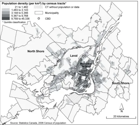
This study focuses on the Island of Montreal (Canada), which, in 2006, was home to 1.85 million people spread across 499 km2. This territory is the central part of the Montreal census metropolitan area (CMA), which is the second most populous metropolis in Canada (with 3.92 million inhabitants). The Island of Montreal represents the most densely populated area of the CMA (Figure 1). We have only considered the Island of Montreal because air pollution data were only available for that geographic area. The Island of Montreal is also an area of interest due to the presence there of the primary sources of pollutants from the road transportation network that enables users to travel to the metropolitan area’s main employment centres, in particular (Crouse et al., 2009b). It is also important to analyze the spatial distribution of environmental nuisances from road transportation given the continual increases in traffic volumes on the Island of Montreal’s main road network since the 1990s (MTQ, 2013). Finally, the socioeconomic profile of the population of the Island of Montreal differs from that in the metropolitan area’s suburbs, in that it includes higher proportions of low-income individuals and visible minorities.
3. Methodological approach
3.1 Study area, targeted groups, and scale of analysis
This study focuses on the Island of Montreal (Canada), which, in 2006, was home to 1.85 million people spread across 499 km2. This territory is the central part of the Montreal census metropolitan area (CMA), which is the second most populous metropolis in Canada (with 3.92 million inhabitants). The Island of Montreal represents the most densely populated area of the CMA (Figure 1). We have only considered the Island of Montreal because air pollution data were only available for that geographic area. The Island of Montreal is also an area of interest due to the presence there of the primary sources of pollutants from the road transportation network that enables users to travel to the metropolitan area’s main employment centres, in particular (Crouse et al., 2009b). It is also important to analyze the spatial distribution of environmental nuisances from road transportation given the continual increases in traffic volumes on the Island of Montreal’s main road network since the 1990s (MTQ, 2013). Finally, the socioeconomic profile of the population of the Island of Montreal differs from that in the metropolitan area’s suburbs, in that it includes higher proportions of low-income individuals and visible minorities.
Research in the field of environmental justice initially concentrated on the presence of environmental hazards in neighbourhoods dominated by poor populations or specific racial groups. Today, researchers are introducing new social categories (Walker, 2009) defined by age, level of disability, or gender (Buckinham and Kulcur, 2009). Walker (2009) suggests that different categories of people be taken into account, especially owing to differentiated vulnerabilities that vary from one group to another.
Our analysis of environmental equity focuses on the low-income population, visible minorities, children under 15 years old, and people aged 65 and older. The first variable represents individuals living in households spending 20% or more of their total before-tax income on food, shelter and clothing, compared with the average Canadian equivalent household (Statistics-Canada, 2006). Visible minorities refer to “persons, other than Aboriginal peoples, who are non-Caucasian in race or non-white in colour” (Statistics Canada, 2006: 116). The numbers of individuals in these groups and for the total population were extracted by Statistics Canada from the 2006 census at the “Dissemination Area” (DA) scale. The DA is the most accurate unit of analysis on which socioeconomic data are available. Generally, 400 to 700 people reside in a DA, and this spatial unit corresponds to a small area composed of one or more neighbouring blocks (Statistics-Canada, 2011).
Determining the existence of environmental inequity for a given group requires analysis at a fine spatial scale, since pollution levels can vary greatly at the scale of a neighbourhood. As a result, we selected the city block (dissemination block) as a spatial unit of analysis. Generally, a city block has a population of less than 300 people, and a few of these spatial units are included in one DA. It should be noted, however, that Statistics Canada only provides data on the total population and the number of dwellings at the city block scale. To address this issue, we estimated the numbers of each group consistent with the approach recently put forward by Pham et al. (2012) at the city block level:
𝑡
𝑖= 𝑡
𝑎𝑇
𝑖𝑇
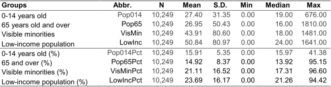
𝑎where ti represents the estimated population of the group (the low-income population, for example) in the block, ta the group’s population in the dissemination area, and Ti and Ta the total population in the block and in the dissemination area respectively. The summary statistics for the socioeconomic variables analyzed at the city block level are reported in Table 1.
Table 1. Univariate statistics of studied groups at the city block scale
Groups Abbr. N Mean S.D. Min Median Max
0-14 years old Pop014 10,249 27.40 31.35 0.00 19.00 676.00
65 years old and over Pop65 10,249 26.95 50.43 0.00 16.00 1810.00
Visible minorities VisMin 10,249 43.91 80.60 0.00 18.00 1481.00
Low-income population LowInc 10,249 50.84 80.97 0.00 24.00 1641.00 0-14 years old (%) Pop014Pct 10,249 15.91 5.35 0.00 15.97 41.38
65 and over (%) Pop65Pct 10,249 14.92 8.37 0.00 13.92 95.15 Visible minorities (%) VisMinPct 10,249 21.11 16.52 0.00 17.31 96.60 Low-income population (%) LowIncPct 10,249 23.69 16.17 0.00 21.26 94.42
3.2 Air pollution indicators
We constructed three kinds of air pollution indicators for the Island of Montreal. The first kind of indicators is based on the typology of Montreal’s roads and highways produced in 2006. The second group of indicators is based on a mathematical model developed by the Quebec Ministry of Transportation in 2011. The third type of indicators was developed by using a land-use regression model created in 2006 at a fine spatial resolution. We describe these three categories of indicators below. The summary statistics for the air pollution indicators calculated at the city block level are reported in Table 2.
Table 2. Univariate statistics of the pollutant indicators at the city block scale
Indicator Abbr. N Mean S.D. P25 P50 P75
Proximity indicators to major roads
A. Highways (metres) Highways 10249 30.88 133.03 0.00 0.00 0.00
B. Collectors or arterials (metres) CollExp 10249 391.52 374.76 0.00 352.31 660.50 C. Highways and collectors (metres) HCE 10249 422.40 417.47 0 361.90 692.36 Pollutant indicators from MOTREM model
D. CO concentration CO 9023 3331.91 6272.85 876.08 1634.51 3113.98
E. NOx concentration NOx 9023 362.62 756.87 86.78 157.75 312.81
F. PM2.5 concentration PM2.5 9023 6.97 14.40 1.62 2.97 5.95
Pollutant indicator from land-use regression
G. NO2 concentration NO2 10249 11.80 2.63 9.79 11.37 13.77
S.D.: Standard deviation; P25: first quartile; P50: median; P75: third quartile.
3.2.1 Indicators of proximity to major roads
To construct our first type of indicators of exposure to ambient pollution, we proceeded as follows. Based on road network data for the Island of Montreal (Geobase), we constructed indices of road typology in buffer zones within a 200-metre radius of the centroids of city blocks, specifically: 1) the lengths of highway sections within the buffer zone; 2) the lengths of
secondary roads—collector, arterial and express roads—within the buffer zone; and, finally, 3) the lengths of highways and secondary roads within the buffer zone.
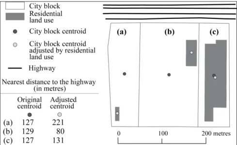
The selected distance was 200 m, since the effects of air pollutants are rarely experienced beyond this distance (Brugge et al., 2007). It is also worth noting that to improve the accuracy of these measurements, the location of the city block centroid was adjusted according to the occupation of residential land, as illustrated in Figure 2. These operations were performed in GIS using ArcGIS version 10 (ESRI, 2011).
Figure 2. Adjustment of location for the city block centroid.
3.2.2 Pollution indicators obtained through mathematical modelling
For pollution indicators obtained through mathematical modelling, we used data from Montreal’s regional MOTREM transportation model developed by the provincial Ministry of Transportation in 2011. MOTREM modelled the levels of three pollutants (i.e., CO, NOx and PM2.5) over 12,691 road sections on the Island of Montreal at five times during a normal fall day in 2011: morning peak hours (6:30 a.m. to 9:30 a.m.), daytime (9:30 a.m. to 3:30 p.m.), afternoon peak hours (3:30 p.m. to 6:30 p.m.), evening (6:30 p.m. to 12:00 a.m.), and night (12:00 a.m. to 6:30 a.m.). These 12,691 road sections cover the entire Island of Montreal, and represent a sample of 45% of the total length of the Montreal road network. The parameters integrated into the MOTREM model also include traffic volumes, vehicle typology, road geometry, and average meteorological conditions (MTQ, 2011).
Based on the MOTREM model, we constructed three air pollution indicators, namely, the average concentration of each pollutant (CO, NOx, and PM2.5) within a 200-metre radius of the adjusted city block centroid. This exercise was performed in two steps. First, we calculated
pollutant concentrations for each period. For example, for period t, the CO measurement within the 200-metre buffer zone around the adjusted city block centroid is calculated as follows: COit = Σ(ls COs/ L)
where COit is the measurement of pollutant CO within buffer zone i for period of the day t, ls is
the road section length included within the buffer zone, COs is the measurement of this pollutant that the model attributes to the section, and L is the total length of the network for which modelling within the zone was performed. Next, we carried out a weighted summation according to the number of hours in each period as follows:
COit = Σ(3COAm peak + 6.5CODay +3COPm peak + 5.5COEvening +6CONight)/24
where COit represents the measurement of CO pollution for the entire day. These air pollution indicators were calculated in only 9,023 city blocks, because no pollutant measurements were available in the spatial units that include local streets exclusively.
3.2.3 Pollution indicators obtained through land-use regression
As reported previously, Crouse et al. (2009a) collected samples of NO2 concentrations during the months of August and December 2005 and May 2006 at more than 133 locations across the Island of Montreal and used these to generate a land-use regression model at a spatial resolution of 5 m. We then used the resulting exposure surface to calculate the average NO2 concentration within a 200-metre distance from each of 10,249 city block centroids where the total population of these city blocks was above 0.
3.3 Statistical analyses to measure environmental inequity
Once all of the indicators are generated for the three types of techniques, i.e., the lengths of major roads, mathematical modelling, and land-use regression, the first step is to assess the association between these indicators by using the Spearman’s rank correlation coefficient. Then, to determine whether environmental inequities exist in relation to our four targeted groups (low-income individuals, members of visible minorities, young people, and the elderly), we conducted four statistical analyses largely used in studies on environmental equity (Apparicio et al., 2010; Briggs et al., 2008; Kingham et al., 2007; Pham et al., 2012). First, a T-test between each group and the rest of the population is performed, in this case to compare their respective averages in terms of pollution indicators (for example, between the population under 15 years old and the population over 15 years old). Secondly, environmental equity is often assessed using the proportion of targeted groups within the total population of given
spatial units. In this vein, we calculated the Spearman’s rank correlation coefficients to verify the existence of significant linear relationships between the proportions of the four studied groups and the seven indicators of pollution exposure. Thirdly, we compared the averages of extreme quintiles based on a T-test (quintile 1 versus quintile 5 in the percentage of the low-income population, for example), an exercise conducted, among others, by Kingham et al. (2007) and Briggs et al. (2008). These analyses were performed in SAS version 9.2 (SAS Institute Inc).
Finally, several multivariate regression analyses were performed, with each of the seven pollution indicators as the dependent variable in each case and the four population groups as the independent variables. We were thus attempting to see whether the associations between the different pollution indicators and a given population group were significant once we had controlled for the proportions of the other three population groups. A number of studies on environmental equity have however shown the spatial dependence of conventional regression models, whether in terms of dependent variables relating to air pollution (Buzzelli, 2003; Chakraborty, 2009), or in terms of those relating to the presence of urban vegetation (Pham et al., 2013; Pham et al., 2012). As we wanted to control for spatial dependence, we constructed two spatial autoregressive models, i.e., the spatial lag and spatial error models (Anselin, 2009). Because city blocks in Montreal are mostly regular and have similar sizes and shapes, we used a row standardized Queen contiguity matrix. For each pollution indicator model, the choice of either spatial lag or spatial error was based on the value of Moran’s I and the Lagrange Multiplier and Robust Lagrange Multiplier (LM and Robust LM) tests calculated using the residuals from the OLS models (Anselin, 2005). The spatial regressions were computed in R by using the spdep library (Bivand, 2013).
4. Results
4.1 Comparison of the pollution indicators
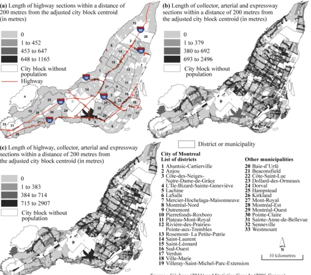
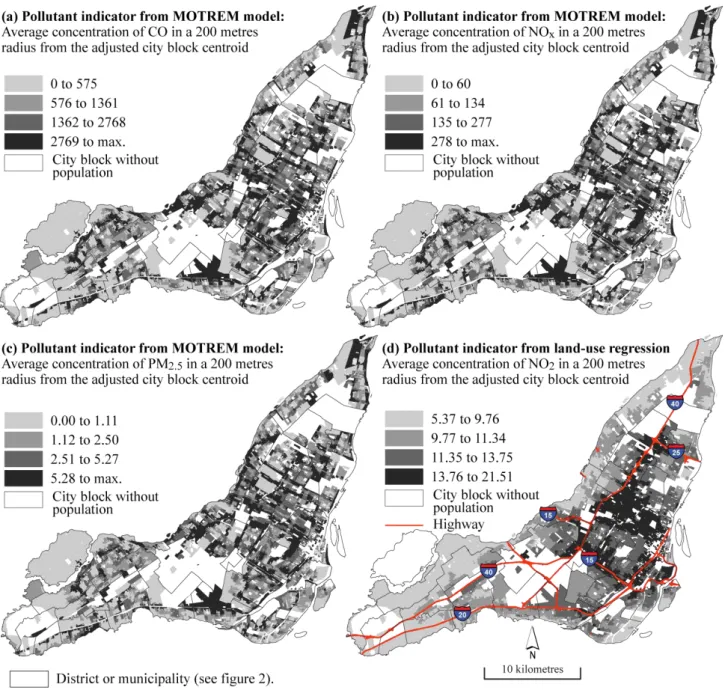
The city blocks exhibiting the greatest lengths of collector streets are mainly located in the city core (Figure 3.b). As for the mathematical modelling (MOTREM model), the highest concentrations of the three pollutants were located in city blocks near the highway network and the main roads that cross Montreal running north and south (Figures 4.a to 4.c). Finally, the NO2 indicator generated by land-use regression is fairly high in areas near the intersections of two or more highways, along highways 40 and 15, and in the city’s central boroughs (Figure 4.d).
Figure 3. The three indicators of proximity to major roads calculated at the city block scale, Island of Montreal.
Figure 4. The three indicators of pollution modeled or measured at the city block scale, Island of Montreal.
To compare the seven indicators, we calculated Spearman’s rank correlation coefficients (Table 3). Overall, with the exception of correlations between the three indicators from mathematical modelling, which are quite strong (i.e., r = >0.95), all other correlations are moderate or low (i.e., ranging from 0.13 to 0.50), but significant (p<0.0001). More specifically, first, the correlations between the indicators of the lengths of highways and secondary roads and the pollution indicators from the MOTREM model are moderate (ranging from r = 0.40 to 0.50 in absolute value). This can be explained by the intrinsic construction of the MOTREM model, i.e., the parameters used: namely, average speed, number of traffic lanes, traffic data volumes and the proportion of heavy vehicles. Second, the correlations are relatively low (r =
0.20 to 0.30 in absolute value) between the indicators of the lengths of major roads and the pollution indicators from the MOTREM model in relation to the land-use regression indicator (NO2).
Table 3. Spearman correlation coefficients between the pollution indicators
Length of major roads MOTREM model regression Land-use
Indicators A B C D E F G A Highways -- 0.134 0.322 0.400 0.407 0.405 0.195 B CollExp 0.134 -- 0.970 0.400 0.410 0.423 0.263 C HCE 0.322 0.970 -- 0.479 0.490 0.502 0.282 D CO 0.400 0.400 0.479 -- 0.977 0.963 0.222 E NOx 0.407 0.410 0.490 0.977 -- 0.995 0.224 F PM2.5 0.405 0.423 0.502 0.963 0.995 -- 0.213 G NO2 0.195 0.263 0.282 0.222 0.224 0.213 --
Highways: length of highways by city block (in metres); CollExp: length of collector, arterial and express roads (in metres) by city block; HCE: length of highways, collector, arterial and express roads (in metres) by city block; CO, NOx and PM2.5: mean concentration in (grams per kilometre) of each pollutant by city block; NO2: mean concentration (in ppb) of NO2 by city block.
All the values are significant ( p<0.0001). N=10,249 for Highways, CollExp and HCE. N=9,023 for CO, CO, NOx and PM2.5.
4.2 Determining environmental inequity
Comparison of averages between the groups and the rest of the population (T-test)
We carried out a T-test to compare the average of the seven indicators weighted by the number of people in each group (compared with the average for the rest of the population (Table 4). We found no substantial differences in absolute exposures between groups based on any of the seven indicators, although the targeted groups generally had slightly higher exposures. The greatest differences between groups were observed for the low-income population (versus the non-low-income population). For example, the average NO2 concentration weighted by the low-income population was 12.87 parts per billion (ppb) (95% CI: 12.82 ppb to 12.92 ppb) versus 12.07 ppb (95% CI: 12.01 ppb to 12.12 ppb) for the non-low-income population, for a difference of 0.80 ppb. The average length of highways and secondary roads in metres weighted by the low-income population was 494 m (95% CI: 486 m to 503 m) versus 423 m (95% CI: 415 m to 431 m) for the rest of the population, for a difference of 71 m. There was no significant difference in terms of exposure to the modelled pollutants (CO, NOx and PM2.5) for young people and the elderly, although it is worth noting the lower and significant exposure for the measured pollutant (NO2) for both of these groups. The averages for highways are likewise non-significant for these two age groups.
Table 4. Means of pollutant indicators from the T-test for the four studied groups and the rest of the population Highways (metres)* Collectors, arterials and express roads (metres)
Mean Difference Mean Difference
Group 1 (G1) Group 2 (G2) G1 G2 Diff P G1 G2 Diff P
0-14 years old ˃ 15 years old 30.8 29.1 1.7 0.372 382.6 420.0 -37.3 0.000 65 years old and over less than 65 years old 31.7 28.9 2.8 0.099 425.6 412.1 13.5 0.010 Visible minorities No visible minorities 39.3 26.0 13.3 0.000 425.3 410.5 14.8 0.005 Low-income population No low-income population 34.0 27.4 6.6 0.000 460.4 395.3 65.1 0.000
HCE (metres) CO*( μg/m-3)
0-14 years old ˃ 15 years old 413.4 449.0 -35.6 0.000 3284.2 3217.5 66.7 0.099 65 years old and over less than 65 years old 457.3 441.0 16.3 0.004 3232.2 3226.8 5.3 0.110 Visible minorities No visible minorities 464.6 436.5 28.1 0.000 3656.9 3080.9 576.0 0.000 Low-income population No low-income population 494.4 422.7 71.7 0.000 3316.6 3189.1 127.5 0.000
NOx*( μg/m-3) PM2.5*( μg/m-3)
0-14 years old ˃ 15 years old 362.0 348.2 13.7 0.464 7.04 6.75 0.29 0.902 65 years old and over less than 65 years old 350.3 350.3 0.0 0.346 6.79 6.79 0.00 0.765 Visible minorities No visible minorities 407.1 330.9 76.2 0.000 7.99 6.38 1.61 0.000 Low-income population No low-income population 363.1 344.8 18.3 0.000 7.08 6.67 0.41 0.000
NO2 (ppb)
0-14 years old ˃ 15 years old 12.10 12.34 -0.24 0.000 65 years old and over less than 65 years old 12.10 12.33 -0.23 0.000 Visible minorities No visible minorities 12.61 12.20 0.41 0.000 Low-income population No low-income population 12.87 12.07 0.80 0.000
If the variances of the two groups are unequal (with P<0.05), the Satterthwaite variance estimator is used for the T-test; otherwise, the pooled variance estimator is used.
* For the four indicators, the p-value is computed after transformation of the variable due to non-normality. However, the mean for each indicator is displayed at the original scale to facilitate interpretation.
Correlation between pollutants and group proportions
We then calculated Spearman’s rank correlation coefficients to verify the existence of significant linear relationships between the percentages of the four studied groups across the seven indicators of pollution exposure (Table 5). Here, we found moderate, positive associations between the proportion of low-income individuals and: 1) the lengths of collector roads, arteries and express roads (r = 0.330, 95% CI: 0.312 to 0.347); 2) the total lengths of highways and secondary roads (r = 0.321, 95% CI: 0.304 to 0.339); and 3) the NO2 level (r = 0.436, 95% CI: 0.422 to 0.453). We also found a moderate, negative association between the proportion of young people and the NO2 level (r = -0.301, 95% CI: -0.318 to -0.283), which indicates that this group benefits from an advantageous situation. Another observation is that the correlations are all positive and significant between the seven indicators and the percentages of the low-income population and members of visible minorities, which suggests a situation of inequity, although fairly low, for these two groups.
Table 5. Spearman coefficients between the pollution indicators and the presence of different groups by city block
Group
Length of major roads MOTREM model Land-use regression
Highways CollExp HCE CO NOx PM2.5 NO2
0-14 years old (%) 0.013 -0.271 -0.257 -0.069 -0.056 -0.052 -0.301 65 years old and over (%) 0.020 -0.024 -0.016 -0.030 -0.016 -0.013 -0.086 Visible minorities (%) 0.083 0.134 0.135 0.094 0.129 0.139 0.121 Low-income population (%) 0.055 0.330 0.321 0.120 0.146 0.153 0.436 Bold: significant at the level of P<0.0001. N=10249 for Highways, CollExp and HCE N=9023 for CO, NOx and PM2.5.
Comparison of averages between the extreme quintiles of group proportions
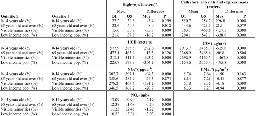
As the Spearman’s rank correlation coefficients are globally moderate, it is possible that the associations between the proportions of the different groups and the pollution indicators are not linear. Consequently, in cases like this, we suggest a final analysis aiming to compare the averages of extreme quintiles based on a T-test. Here, the output of this analysis, shown in Table 6, further suggests some environmental inequity for the low-income population and visible minorities. For example, the NO2 average for the highest quintile in the percentage of low-income individuals is 13.24 ppb (95% CI: 13.14 ppb to 13.35 ppb) versus 10.22 ppb (95% CI: 10.15 ppb to 10.31 ppb) for the lowest quintile, representing a difference of 3.02 ppb in the concentration of this pollutant. In comparison, the gap between NO2 averages weighted by the number of low-income individuals and those not belonging to this category was only 0.80 ppb (Table 3). The results are similar for the group of visible minorities and the average for the pollutant NOx—which is almost twice as low in the lowest quintile (278.2 μg/m-3, 95% CI: 245.7 μg/m-3 to 310.7 μg/m-3) as in the highest (469.3 μg/m-3, 95% CI: 432.3 μg/m-3 to 506.4 μg/m -3), for a difference of 191.1 μg/m-3—as well as the average for the pollutant CO, for which the discrepancy between extreme quintiles is -1,467.8 μg/m-3. These results are consistent with those for the average lengths of highways and secondary roads. Finally, as with the two preceding analyses, it appears that elderly people are not subject to inequity: only one T-test is significant (at p <0.01): namely, the T-test for NO2. Furthermore, the value for pollution is lower in the highest quintile of seniors than in the lowest. Lastly, city blocks with a high concentration of young people show lower levels of NO2 pollution and a lower presence of main road networks other than highways. However, for young people, the results appear contradictory for two of the modelled pollutants (CO and NOx): the averages are higher for the last quintile, which represents an inverse relationship compared with the averages observed with the Spearman’s rank correlation coefficients, which were slightly negative.
Table 6. Comparison of values for pollutant indicators associated with the minimal and maximal quintiles of the studied groups
Highways (meters)* Collectors, arterials and express roads (meters)
Mean Difference Mean Difference
Quintile 1 Quintile 5 Q1 Q5 Moy P Q1 Q5 Moy P
0-14 years old (%) 0-14 years old (%) 27.2 30.6 -3.4 0.299 550.7 254.7 296.0 0.000 65 years old and over (%) 65 years old and over (%) 32.6 40.6 -8.0 0.012 444.6 423.3 21.3 0.079 Visible minorities (%) Visible minorities (%) 15.0 50.8 -35.8 0.000 303.1 460.6 -157.5 0.000 Low income pop. (%) Low income pop. (%) 21.6 37.8 -16.2 0.000 204.1 542.1 -338.0 0.000
HCE (meters) CO*( μg/m-3)
0-14 years old (%) 0-14 years old (%) 577.9 285.3 292.6 0.000 2973.7 3488.7 -515.0 0.000 65 years old and over (%) 65 years old and over (%) 477.1 463.9 13.3 0.326 3368.9 3465.6 -96.8 0.504 Visible minorities (%) Visible minorities (%) 318.1 511.4 -193.2 0.000 2692.9 4160.7 -1467.8 0.000 Low income pop. (%) Low income pop. (%) 225.7 579.9 -354.2 0.000 3154.6 3350.4 -195.8 0.000
NOx*( μg/m-3) PM2.5*( μg/m-3)
0-14 years old (%) 0-14 years old (%) 302.7 397.1 -94.3 0.000 5.74 7.64 -1.90 0.163 65 years old and over (%) 65 years old and over (%) 358.6 382.9 -24.3 0.874 6.84 7.26 -0.41 0.877 Visible minorities (%) Visible minorities (%) 278.2 469.3 -191.2 0.000 5.18 9.36 -4.18 0.000 Low income pop. (%) Low income pop. (%) 346.5 367.2 -20.7 0.000 6.33 7.27 -0.94 0.000
NO2 (ppb)
0-14 years old (%) 0-14 years old (%) 13.09 10.90 2.19 0.000 65 years old and over (%) 65 years old and over (%) 12.38 11.68 0.70 0.000 Visible minorities (%) Visible minorities (%) 11.23 12.45 -1.22 0.000 Low income pop. (%) Low income pop. (%) 10.22 13.24 -3.02 0.000
If the variances of the two groups are unequal (with P<0.05), the Satterthwaite variance estimator is used for the T-test; otherwise, the pooled variance estimator is used.
* For the four indicators, the P-value is computed after transformation of the variable due to no-normality. However, the mean for each indicator is displayed at the original scale to facilitate interpretation.
Multivariate analysis
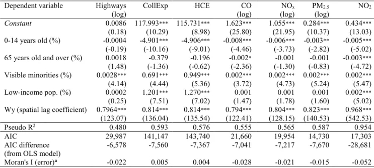
Due to lack of space, we are reporting only the fit diagnostic and the diagnostic for spatial dependence for the conventional model (Table 7). The Moran’s I values calculated among residuals clearly show the spatial dependence of the OLS models. Moreover, the higher values for the Lagrange Multiplier and Robust Lagrange Multiplier tests for lag compared with those for error suggest the relevance of using a spatial error model, for all seven pollution indicators. It should first be noted that the AIC values show that the spatial lag models represent a marked improvement over the OLS models. Globally, the results of the spatial models corroborate those obtained from the bivariate analyses (Table 8). Young people under 15 years old are in quite a favourable situation since they present significant and negative coefficients with six of the seven pollution indicators. This means that, as the proportion of this group increases in a city block, there are fewer major roads and lower concentrations of pollutant emissions. The percentage of people aged 65 and older is only negatively and significantly associated with the NO2 indicator. Conversely, all the correlations are positive and significant between the percentage of visible minorities per city block and the seven pollution indicators. On the other hand, only three coefficients are significant and positive between the percentage of low-income individuals and: the lengths of major roads and highways, and the NO2 concentrations. It is also worth noting that the coefficients for the first two indicators—the lengths of major
roads and highways—are higher for the percentage of low-income individuals than for the percentage of visible minorities.
Table 7. Diagnostic of the ordinary least squares regressions of the pollution indicators Dependent
variable Highways (log) CollExp HCE (log) CO (log) NOx PM(log) 2.5 NO2 OLS fit diagnostic
R2 0.010 0.147 0.129 0.024 0.028 0.029 0.245
Adjusted R2 0.010 0.147 0.128 0.023 0.028 0.028 0.245 F statistic 26.73*** 441.60*** 377.70*** 54.70*** 65.02*** 66.75*** 831.60***
AIC 36,565 148,707 151,107 28,701 27,171 22,400 45,984 Diagnostic for spatial dependence of the OLS models
Moran's I (error)a 0.561*** 0.585*** 0.577*** 0.650*** 0.650*** 0.658*** 0.886***
LM (lag) 7,742*** 8,517*** 8,269 *** 8,268*** 8,278 *** 8,483*** 19,635***
LM (error) 7,719*** 8,378*** 8,148*** 8,234*** 8,243*** 8,446*** 19,219***
RLM (lag) 24.99*** 215.03*** 184.14*** 40.98*** 45.11*** 48.13*** 798.87***
RLM (error) 1.47 76.29*** 63.14*** 6.92** 10.57*** 11.43*** 382.05*** a Moran’s I is computed with a row standardized Queen matrix; P is obtained with a randomization procedure
(999 permutations).
LM: Lagrange Multiplier. RLM: Robust Lagrange Multiplier. * p < 0.05. ** p < 0.01. *** p < 0.001.
Table 8. Spatial lag regressions of the pollution indicators Dependent variable Highways
(log) CollExp HCE (log) CO (log) NOx PM(log) 2.5 NO2
Constant 0.0086
(0.18) 117.993(10.29) *** 115.731(8.98) *** 1.623(25.80) *** 1.055(21.95) *** 0.284(10.37) *** 0.434(13.03) *** 0-14 years old (%) -0.0004
(-0.19) -4.901(-10.16) *** -4.906(-9.01) *** -0.008(-4.46) *** -0.006(-3.73) *** -0.003(-2.82) ** -0.005(-5.02) *** 65 years old and over (%) 0.0018
(1.48) (-1.36) -0.379 (-0.62) -0.196 -0.002(-2.36) * (-1.30) -0.001 (-0.83) -0.001 -0.003(-4.72) *** Visible minorities (%) 0.0028***
(4.14) 0.691(4.44) *** 0.949(5.36) *** 0.002(3.72) *** 0.002(4.73) *** 0.002(5.24) *** 0.002(5.47) *** Low-income pop. (%) 0.0002
(0.25) 1.201(7.51) *** 1.270(7.02) *** (1.47) 0.001 (1.78) 0.001 (1.60) 0.001 0.002(5.02) *** Wy (spatial lag coefficient) 0.7964***
(123.07) 0.814(136.04) *** 0.814(135.54) *** 0.794(122.41) *** 0.804(128.15) *** 0.823(140.53) *** 0.968(542.53) ***
Pseudo R2 0.480 0.593 0.576 0.555 0.565 0.587 0.954
AIC 29,987 141,147 143,740 21,660 19,954 14,730 17,303
AIC difference
(from OLS model) -6,578 -7,560 -7,367 -7,041 -7,217 -7,670 -28,681 Moran's I (error)a -0.022 0.005 0.004 -0.028 -0.021 -0.015 -0.052 a Moran’s I is computed with a row standardized Queen matrix; P is obtained with a randomization procedure (999
permutations).
5. Discussion
Our results regarding environmental equity with three different methods of exposure assessment for four different population groups in Montreal are consistent with those of previous studies. In particular, our results for each group corroborate those reported by Crouse et al. (2009b) at the level of census tracts in Montreal. In addition, we offer a broader view of the environmental equity diagnosis for these four groups by considering multiple exposure estimates, while other studies generally use only one indicator to evaluate a situation of
inequity. First, the bivariate analysis demonstrated a higher exposure to estimates of pollution for the low-income population and, to a lesser extent, for visible minorities. Secondly, as in other studies (Brainard et al., 2002; Chakraborty, 2009; Mitchell and Dorling, 2003), we found no inequity for young people or the elderly, although we did not introduce control variables, such as deprivation. Our results for these four groups can largely be explained by the urban landscape and social geography of Montreal.
To begin with, it is not surprising that the low-income population are more exposed to pollutants since they are concentrated in Montreal’s central neighbourhoods (Apparicio and Seguin, 2006). These spaces are above all characterized by higher residential density, the diversity of urban functions, and the greater concentration and lengths of collector roads, arteries, expressways, and highways that link together the main poles of attraction on the Island of Montreal, as well as the access toward the bridges and the major suburbs of the CMA, hence the higher traffic data volumes. So the geography of road transportation and the location of this group in the centre of the Island of Montreal explain, in part at least, the higher concentration of pollutants for this group (Carrier et al., 2014). The values of some of the pollution indicators are thus more strongly explained by the presence of individuals from low-income households.
Visible minorities on the Island of Montreal were found to have only slightly higher exposures than non-visible minorities. This finding is consistent with those of two other Canadian studies conducted in Hamilton and Toronto (i.e., the studies by Buzzelli and Jerrett (2004, 2007). Moreover, the lower degree of ethnic residential segregation in large Canadian cities compared with their American counterparts might well explain these significantly lower levels of environmental inequity in terms of pollution (Buzzelli and Jerrett, 2004).
Young people under 15 years old appear to reside in areas with fewer major roads and lower pollution levels, especially as reflected by NO2 measurements. Since the 1950s, the presence of young people under 15 years old has been falling in the city’s central boroughs while it has considerably increased in the suburbs on the outskirts of the Island of Montreal (Apparicio et al., 2010). These areas are characterized by low urban density and low functional diversity— the vast majority of homes being single-family houses—along with a roadway network organized so as to serve residential neighbourhoods, thus minimizing the presence of major roads.
Finally, individuals aged 65 and older residing on the Island of Montreal do not appear to be faced with environmental inequity either. This is not surprising, since a recent study on the evolving distribution of elderly people in Montreal from 1981 to 2006 has demonstrated that this group has become decentralized (Séguin et al., 2013). In other words, the elderly are
increasingly dispersed across the island and, in particular, they are increasingly present in the inner suburbs.
Some authors focusing on environmental equity have recently measured the difference associated with the likelihood of developing certain illnesses within the same group based on the combination of two socioeconomic variables, such as, for example, age and ethnic origin (Collins et al., 2011). So it would have been interesting here to compare the differences in pollutant concentrations and the lengths of major roads measured between individuals in the same group: for example, young people under 15 years old that are not low-income individuals and those in low-income situations. The use of census microdata would have been necessary for this type of analysis. However, the numbers of the groups considered are low at the city block level, which does not enable us, moreover, to perform comparative analyses combining two socioeconomic variables, as done by Collins et al. (2011).
5.1 Environmental inequity, pollutant exposure inequity or environmental
injustice?
One of the main issues in environmental equity is to assess the health risk associated with living in a residential area with higher concentrations of air pollutants (Walker, 2011). The objective then becomes to establish whether the targeted groups are exposed to pollutant concentrations that can affect health (Janssen and Mehta, 2006). The World Health Organization (WHO) has determined that annual concentrations of NO2 should not exceed 40 μg/m-3 (Forastiere et al., 2006). The average concentration of this pollutant in our study area is 13.24 ppb in city blocks with high concentrations of the low-income population (the last quintile), which is equivalent to 24.62 μg/m-3, i.e., a level much lower than the threshold set by the WHO.
This finding nuances the observation of environmental inequity in connection with the low-income population in Montreal. Although lower-low-income individuals tend to live in more polluted areas than the rest of the population, the concentration is deemed “not harmful” to health, according to the World Health Organization. In addition, the low-income population that reside near the downtown area can benefit from certain amenities related to their location. Apparicio and Séguin (2010) have demonstrated that central neighbourhoods, especially deprived ones, have better access to services and equipment than those on the periphery of the Island of Montreal. Moreover, residential proximity to major roads sometimes offers better access to public transportation networks, thus improving mobility for households without vehicles (Feitelson, 2002). However, it should also be kept in mind that, owing to their socioeconomic
position and hence their limited mobility, the low-income population have fewer resources to protect themselves from high concentrations of pollutants in their areas of residence (O'Neill et al., 2003). Conversely, more wealthy households that reside in significantly more polluted environments can more easily get out of the city: for example, by acquiring a second house (Forastiere et al., 2007). It therefore seems important to consider several elements relating to the urban environment before making a diagnosis of environmental inequity for a given group within the population. Indeed, studies on environmental equity, including this one, have tended to focus on one single element in the urban environment, a fact that has recently come under criticism (Kruize et al., 2007; Walker, 2011).
Finally, environmental equity is often confused with environmental justice. The distinction between the two concepts, according to Cutter (1995), is that environmental justice involves more than an equal sharing of harmful environmental agents. It must, for instance, provide sufficient protection for various population groups exposed to such hazards (Perlin et al., 1995). Walker and Bulkeley (2006) have also noted that “an unequal distribution of environmental bads by itself may not necessarily be unjust (Walker et al., 2005)—it is rather the ‘fairness’ of the processes through which the distribution has occurred and the possibilities which individuals and communities have to avoid or ameliorate risk, which are important” (Walker and Bulkeley, 2006). So the data brought together in the context of this article do not enable us to demonstrate that the situation of inequity existing in regard to low-income households is the result of discriminatory processes leading to environmental injustice.
5.2 Comparability of the three techniques used
We have shown that moderate or weak correlations exist between the three techniques used (with Spearman coefficients ranging from 0.20 to 0.50 in absolute value). These findings are consistent with the fact that the spatial association between some groups and an environmental phenomenon could be different if a measure is taken directly or provided through a proxy (Kingham and Dorset, 2011; Maantay et al., 2010; Walker, 2010). This study shows that the assessment of environmental equity differs depending on the choice of the exposure estimate (Bowen, 2002).
At first glance, the most unexpected element is the relatively weak correlation between the measured pollutant (NO2) and the modelled pollutants (CO, NOx, PM2.5) (± 0.20). Because of the typical co-localization of NO2 with the pollutants PM and CO, one might have expected higher correlation coefficients. The results of this study remind us of the differences that may occur between a proxy and a measure taken directly. This situation can be explained in part
by two principal factors. The first has to do with the time frame for data collection. The MOTREM model uses data on traffic data volumes for one day during the fall—a time of year when traffic data volumes are at their highest—while the NO2 data represent an average of measurements collected in the summer, winter and spring. The second explanatory factor has to do with geographical scale: the MOTREM model has a regional scope, while the use of NO2 samplers has a local scope. It should be noted that a number of studies have shown significant spatial variability in pollution at the intra-urban level (Briggs et al., 2000; Jerrett et al., 2005) caused by the interaction between meteorological factors (Seaman, 2000), urban functions, and local particularities of traffic (Crouse et al., 2009a). We did unexpectedly find weak correlations between the NO2 estimates and the indicator of the length of highways (coefficient = 0.195). As some authors have pointed out (Kingham and Dorset, 2011; Maantay et al., 2010), the mere presence of a highway within a 200-metre radius is insufficient to explain NO2 concentrations, since highway sections can have different traffic volumes. In addition, NO2 pollution is generated not only by highways, but also by other road types, especially collector, arterial and express roads.
Finally, revealing a situation of environmental inequity for a given group across all three measurement techniques would clearly demonstrate the existence of this inequity, compared with a traditional approach based on the use of a single method for measuring pollutants. It should be noted that the three statistical analyses performed here have all shown much greater inequity for the low-income population with regard to NO2 exposure than with regard to pollutants modelled at a more regional scale. Indeed, the correlation between this group and NO2 is three times higher compared with the modelled pollutants (0.44 versus values below or equal to 0.15). In a context where the literature on environmental equity seeks to measure health consequences associated with pollutant exposure, the variable of exposure must be as accurate as possible according to the scale of analysis (Walker, 2010). The land-use regression method—which land-uses several elements from the built environment and urban functions, at a fine scale, to predict pollutant levels—therefore appears more appropriate for studies on environmental equity. This is particularly true in light of the existence of micro-spaces of poverty in Montreal (Séguin et al., 2012).
6. Limits of the study
Operationalizing these techniques has shown the approximate level of the pollutants, i.e., their concentration (Janssen and Mehta, 2006). It is important to distinguish between the notions of pollutant concentration and exposure. Exposure has to do with the period of time that an individual spends in an environment and the quantity of pollutants to which the person is
exposed (Janssen and Mehta, 2006). This makes it complex to measure individuals’ actual exposure to pollutants, since it is difficult to ascertain the time period during which they remained at their residence, for example (Kingham and Dorset, 2011; Maantay et al., 2010). In addition, this analysis only takes into account selected pollutants, while individuals may also be exposed to many other pollutants (Crouse et al., 2009a). The Quebec provincial Ministry of Transportation specifies the limitations of its mathematical model: polluting emissions produced by the MOTREM model are at the regional level—since this model includes only the upper hierarchy of the road network—and, as such, these emissions do not necessarily take into account phenomena produced at the micro-local level (MTQ, 2011). Furthermore, the MOTREM model did not estimate pollution for roughly 1,000 city blocks—located mainly in the western suburbs of Montreal, where the proportions of young people are very high—since these areas almost exclusively contain a network of local streets with low traffic data volumes. If values had been assigned to these blocks, they would probably have been very low and would therefore have contributed to lowering or inverting the discrepancy between the extreme quintiles of young people under 15 years old (Table 5).
7. Conclusion
The results of this analysis are consistent with those of a number of studies on environmental equity: the low-income population and, to a lesser extent, visible minorities do tend to reside in more polluted areas. We found these associations to be consistent across seven different estimates of exposure. On the other hand, in Montreal, young people under 15 years old, as well as elderly people, tend to be located in less polluted areas. Yet, while a situation of distributional inequity is associated with pollution in this city, it would be hasty to conclude that this represents a situation of environmental inequity that is highly harmful to the health of the low-income population.
We have also shown that diagnoses of environmental equity relating to air pollution vary from one technique to another. Indeed, the observed inequalities were stronger for the NO2 pollutant indicator than for the other pollutant indicators. We can therefore say that, in general, an erroneous diagnosis of environmental equity may be reported if only one method is used. According to numerous authors (Bowen, 2002; Walker, 2010), it is essential to accurately measure a studied phenomenon in order to properly assess health risks for targeted groups. Although, in the context of this study, the associations were stronger with the land-use regression method, it is difficult for us to conclude that this is the most appropriate technique irrespective of the data, the scale of analysis, and the context of a given study. However, the combined use of different approaches to measure pollutants and their divergent results call
for caution in our diagnosis of environmental equity. Moreover, this shows that more sophisticated measurements have to be developed in order to accurately assess greater pollution exposures for specific social groups.
Acknowledgements
This study has been funded by the Social Sciences and Humanities Research Council of Canada (SSHRC). We thank Mark Goldberg (department of medicine, McGill University) for the provision of the NO2 data pollution. We thank the anonymous reviewers for their careful reading of our manuscript and their many insightful comments and suggestions.
8. References
Amram, O., Abernethy, R., Brauer, M., Davies, H., Allen, R., 2011. Proximity of public elementary schools to major roads in Canadian urban areas. International Journal of Health Geographics 10(68), 1-11.
Anselin, L., 2005. Exploring spatial data with GeoDaTM : A workbook. Spatial Analysis Laboratory, Department of Agricultural and Consumer Economics, University of Illinois. Anselin, L., 2009. Spatial regression, In: Rogerson, I.A.S.F.P.A. (Ed.), The Sage Handbook of Spatial Analysis. Sage, London.
Apparicio, P., Cloutier, M.-S., Séguin, A.-M., Ades, J., 2010. Accessibilité spatiale aux parcs urbains pour les enfants et injustice environnementale : exploration du cas montréalais. Revue Internationale de Géomatique 20(3), 363-389.
Apparicio, P., Seguin, A.-M., 2006. Measuring the accessibility of services and facilities for residents of public housing in Montreal. Urban Studies 43(1), 187-211.
Apparicio, P., Séguin, A.-M., 2010. Accessibility to proximity services in poor areas of the Island of Montreal, Modeling Urban Dynamics: Mobility, Accessibility and Real Estate Value. Wiley.
Apparicio, P., Séguin, A.-M., Naud, D., 2008. The quality of the urban environment around public housing buildings in Montréal: an objective approach based on GIS and multivariate statistical analysis. Social Indicators Research 86(3), 355-380.
Bae, C.H.C., Sandlin, G., Bassok, A., Kim, S., 2007. The exposure of disadvantaged populations in freeway air-pollution sheds: a case study of the Seattle and Portland regions. Environment and Planning B: Planning and Design 34(1), 154-170.
Beckerman, B., Jerrett, J., Brook, J.R., Verma, D.K., Arain, M.A., Finkelstein, M., 2008. Correlation of nitrogen dioxide with other traffic pollutants near a major expressway. Atmospheric Environment 42(2), 275-290.
Bivand, R., 2013. Spdep: Spatial Dependence: Weighting Schemes, Statistics and Models.R Package Ver.0.5-56. .
Bolte, G., Tamburlini, G., Kohlhuber, M., 2009. Environmental inequalities among children in Europe-evaluations of scientific evidence and policy implications. European Journal of Public Health 20(1), 14-20.
Bowen, W., 2002. An analytical review of environmental justice research: what do we really know ? Environmental Management 29(1), 3-15.
Brainard, J., Bateman, I., Lovett, A., Fallon, P., 2002. Modelling environmental equity: access to air quality in Birmingham, England. Environment and Planning A 34(4), 695-716.
Briggs, D., Abellan, J., Fecht, D., 2008. Environmental inequity in England: small area associations between socio-economic status and environmental pollution. Social Science and Medecine 67(10), 1612-1629.
Briggs, D., de Hoogh, C., Gulliver, J., Wills, J., Elliott, P., Kingham, S., 2000. A regression-based method for mapping traffic-related air pollution : application and testing in four contrasting urban environments Science of the Total Environment 253, 151-167.
Brugge, D., Durant, J., Rioux, C., 2007. Near-highway pollutants in motor vehicle exhaust: A review of epidemiologic evidence of cardiac and pulmonary health risks. Environmental Health 6(23), 1-12.
Brulle, R., Pellow, D., 2006. Environmental justice: human health and environmental inequalities. Annual Review of Public Health 27, 103-124.
Brunekreef, B., Holgate, S., 2002. Air Pollution and Health. Lancet 360(9341), 1233-1242. Buckinham, S., Kulcur, R., 2009. Gendered geographies of environmental injustice. Antipode 41(4), 659-683.
Buzzelli, M., 2003. Comparing Proximity Measures of Exposure to Geostatistical Estimates in Environmental Justice Research. Environmental Hazards 5(1), 13-21.
Buzzelli, M., Jerrett, M., 2004. Racial gradients of ambient air pollution exposure in Hamilton, Canada. Environment and Planning A 36(10), 1855-1876.
Buzzelli, M., Jerrett, M., 2007. Geographies of susceptibility and exposure in the city: environmental inequity of traffic-related air pollution in Toronto. Canadian Journal of Regional Science 30(2), 195-210.
Carrier, M., Séguin, A.-M., Apparicio, P., Crouse, D., 2014. Les résidences pour personnes âgées de l’île de Montréal appartenant aux parcs social et privé : une exposition inéquitable à la pollution de l’air ? Cahiers de géographie du Québec (Sous presse).
Cesaroni, G., Badaloni, C., Romano, V., Donato, E., Perucci, C., Forastiere, F., 2010. Socioeconomic position and health status of people who livre near busy roads : the Rome longitudinal study (RoLS). Environmental Health 9(41), 1-12.
Chaix, B., Gustafsson, S., Jerret, M., Kristerson, H., Lithman, T., Boalt, A., Merlo, J., 2006. Children's exposure to nitrogen dioxide in Sweden: investigating environmental injustice in an egalitarian country. Journal of Epidemiology and Community Health 60(3), 234-241.
Chakraborty, J., 2006. Evaluating the environmental justice impacts of transportation improvement projects in the US. Transportation research Part D 11(5), 315-323.
Chakraborty, J., 2009. Automobiles, air toxics, and adverse health risks: environmental inequities in Tampa Bay, Florida. Annals of Association of American Geographers 99(4), 674-697.
Chakraborty, J., Forkenbrock, D., Schweitzer, L., 1999. Using GIS to Assess the Environmental Justice Consequences of Transportation System Changes. Transactions in GIS 3(3), 239-258.
Collins, T., Grineski, S.E., Chakraborty, J., McDonald, Y., 2011. Understanding Environmental Health Inequalities through Comparative Intracategorical Analysis: Racial/ethnic Disparities in Cancer Risks from Air Toxics in El Paso County, Texas. Health & Place 17(1), 335-344.