https://doi.org/10.1007/s00027-018-0573-4
RESEARCH ARTICLE
Seasonal and inter-annual variations in carbon fluxes in a tropical river
system (Tana River, Kenya)
Naomi Geeraert1 · Fred O. Omengo1,2 · Fredrick Tamooh1,3 · Trent R. Marwick1 · Alberto V. Borges4 · Gerard Govers1 · Steven Bouillon1
Received: 2 July 2017 / Accepted: 17 February 2018
© Springer International Publishing AG, part of Springer Nature 2018 Abstract
The hydrological status of river systems is expected to change due to dam operations and climate change. This will affect the riverine fluxes of sediment and carbon (C). In rivers with strong seasonal and inter-annual variability, quantification and extrapolation of sediment and C fluxes can be a challenge as measurement periods are often too short to cover all hydrologi-cal conditions. We studied the dynamics of the Tana River (Kenya) from 2012 to 2014 through daily monitoring of sediment concentrations at three sites (Garissa, Tana River Primate Reserve and Garsen) and daily monitoring of C concentrations in Garissa and Garsen during three distinct seasons. A bootstrap method was applied to calculate the range of sediment and C fluxes as a function of annual discharge by using daily discharge data (1942–2014). Overall, we estimated that on average, sediment and carbon were retained in this 600 km long river section between Garissa to Garsen over the 73 years (i.e., fluxes were higher at the upstream site than downstream): integration over all simulations resulted in an average net retention of sediment (~ 2.9 Mt year− 1), POC (~ 18,000 tC year− 1), DOC (~ 920 tC year− 1) and DIC (~ 1200 tC year− 1). To assess the
impact of hydrological variations, we constructed four different hydrological scenarios over the same period. Although there was significant non-linearity and difference between the C species, our estimates generally predicted a net increase of C retention between the upstream and downstream site when the annual discharge would decrease, for example caused by an increase of irrigation with reservoir water. When simulating an increase in the annual discharge, e.g. as a potential effect of climate change, we predicted a decrease in C retention.
Keywords Carbon fluxes · Tropical rivers · Inter-annual variability · Intra-annual variability · Long term simulations ·
Carbon retention
Introduction
The riverine flux of carbon (C) to the ocean is an important component of the global C budget, and of interest both from a terrestrial perspective (representing a loss of terrestrial
organic C), and from a marine perspective (representing an input of organic and inorganic C). Efforts to constrain these fluxes were initiated several decades ago, and either established relationships between the total annual river flow and the total organic carbon (TOC) load or calculated as the loss of organic carbon (OC) based on the spatial extent of terrestrial ecosystems and their expected areal rate of C loss (Garrels and Mackenzie 1971; Schlesinger and Melack
1981; Degens et al. 1982, 1991; Meybeck 1987). Increas-ingly refined models incorporated global spatial datasets of precipitation, temperature and vegetation (Ludwig et al.
1996), the most recent being the Global Nutrient Export from Watersheds (NEWS and NEWS2) models, which include relationships with ecological, climatic and geomor-phologic characteristics of the catchment (Seitzinger et al.
2005; Mayorga et al. 2010). In recent models, the particulate OC (POC) flux is often estimated based on the sediment
Aquatic Sciences
* Naomi Geeraert
1 Department of Earth and Environmental Sciences, KU
Leuven, Celestijnenlaan 200E, 3001 Louvain, Belgium
2 Kenya Wildlife Service, P.O. Box 40241-00100, Nairobi,
Kenya
3 Department of Zoological Sciences, Kenyatta University, P.O
Box 16778-80100, Mombasa, Kenya
4 Unité d’Océanographie Chimique, Institut de Physique (B5),
flux and the OC% in the solid flux (Ludwig et al. 1996; Beusen et al. 2005), while the dissolved OC (DOC) flux is estimated based on relationships with soil characteristics in the catchment, either through the C/N ratio or through the C content and vegetation cover (Ludwig et al. 1996; Ait-kenhead and McDowell 2000). Inorganic C (IC) fluxes are estimated based on the variation of weathering and erosion-related parameters between and within catchments (Ludwig et al. 1998).
The robustness of these global C flux estimates strongly depends on the reliability and representativeness of the underlying datasets. The historical paucity of datasets rep-resenting tropical river systems has been a strong impetus for the burgeoning research on sediment and C fluxes within these systems over the past decade, and has also witnessed a broadening geographical coverage. While the Amazon has traditionally functioned as the archetype for tropical riv-ers (Richey et al. 2002; Moreira-Turcq et al. 2003, 2013; Mayorga et al. 2005; Abril et al. 2014), there has been an increase in data availability from other systems in Latin-America (Depetris and Kempe 1993; Laraque et al. 2013; Mora et al. 2014), as well as a range of systems in Asia (Sarin et al. 2002; Aldrian et al. 2008; Bird et al. 2008; Zhou et al. 2013), small islands (Wiegner et al. 2009; Lloret et al.
2011), and Africa (Coynel et al. 2005; Brunet et al. 2009; Bouillon et al. 2012; Wang et al. 2013; Zurbrügg et al. 2013; Tamooh et al. 2014; Borges et al. 2015).
Although the spatial extent of river basins where C dynamics have been studied is expanding, the temporal res-olution is often relatively low, with many studies based on a limited number of longitudinal cruises. Monitoring cam-paigns most often achieve only monthly measurements or, in a few cases, biweekly or weekly measurements (e.g. Bouil-lon et al. 2012; Brunet et al. 2009; Tamooh et al. 2014). The monitoring period lasted 1 or 2 years in most of these cases. However, tropical rivers are often characterized by a strong seasonality and a high inter-annual variability (Syvitski et al.
2014), which is difficult to capture with either longitudinal or relatively short monitoring campaigns.
Efforts to unravel the C dynamics of the Tana River (Kenya) experienced an increase in the temporal resolution: from longitudinal surveys (Bouillon et al. 2009; Tamooh et al. 2012, 2013) and monthly sampling efforts in the lower Tana River (Tamooh et al. 2014) to daily samples during three distinct wet seasons (Geeraert et al. 2017). Here, we merged the available data on sediment and C concentration in the lower Tana River (1) to explore the long term sedi-ment and C balance and (2) to assess the impact of hydro-logical changes in C fluxes, irrespective of whether those changes are due to climate change or dam operations.
To achieve this, we first investigated the seasonal distri-bution of the fluxes, as dam operations have been reported to alter the seasonal discharge (Maingi and Marsh 2002).
Subsequently, we looked at the relationship between the annual discharge and the downstream change in C fluxes and C speciation. This information was needed to assess the changes in case the area gets wetter due to climate change or when the discharge decreases due to increased abstraction and evaporation from the reservoir behind the dam. Because our method relied on the identification of two distinct hydro-logical regimes, we started the discussion with identifying the errors that would be induced when failing to recognise the two regimes before we discussed the expected changes.
Methodology
Study area
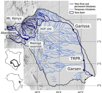
The Tana River, with a length of ca. 1100 km, is the longest river in Kenya (Fig. 1). It originates in the highlands of the Aberdare Mountain Range and Mount Kenya. Five major reservoirs have been built in the upper reaches of the catch-ment of which Masinga Reservoir is the largest (~ 1.56 km3).
A considerably larger dam, the High Grand Falls (HGF) dam (5.7 km3), is planned downstream of the existing dams (Tana
and Athi Rivers Development Authority 2016). Approxi-mately 600 km from the river mouth, the river enters a semi-arid environment, where it starts meandering through a forested floodplain seldom wider than 5 km. Beyond the floodplain, the landscape is characterized by open savannah vegetation. The last 70 km before reaching the Indian Ocean,
Fig. 1 Hill shade map of the Tana River Basin. The insets show Kenya in Africa (bottom left) and the Tana River Basin within Kenya (middle left). (TRPR Tana River Primate Reserve, HGF High Grand Falls dam)
there is a deltaic system with mangrove forests and season-ally flooded grasslands.
The focus of this research is the lower reach of the Tana River, with sampling sites at Garissa, Tana River Primate Reserve (TRPR) and Garsen, measured along the river at 455, 155 and 70 km from the river mouth (Fig. 1). No permanent tributaries are present over this distance, which makes it an ideal setting to compare incoming and outgo-ing fluxes of water, sediment and C (Geeraert et al. 2017). Some “lagas” (temporary rivers) are present, but they are only active for a few days per year.
Precipitation is concentrated within the upper catchment where the average annual rainfall exceeds 1500 mm year− 1,
whereas the average annual precipitation near Garissa is less than 350 mm year− 1. The majority of rainfall occurs
across two wet seasons; the long wet season spanning March through May, and the short wet season which takes place from October to December. Besides the spatial and seasonal variability, the inter-annual variability in the amount of pre-cipitation and the onset and ending of the wet seasons is very high (Indeje et al. 2000).
Long‑term discharge dataset
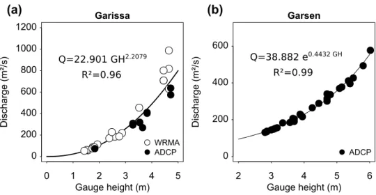
Daily water levels were recorded by government institu-tions (at present the Water Resource Management Author-ity, WRMA) at Garissa and are available either as discharge (from 18th of April, 1941 until January, 2012) or as gauge height (from 1st of April, 2010 until 31st December 2014). A discharge rating curve based on 19 manual measurements (SEBA F1 Universal current meter) by WRMA between 2007 and 2011 and 11 measurements with an Acoustic Dop-pler Current Profiler (ADCP, Teledyne RiverRay, our data) in 2012 and 2013, was constructed to convert the recent measurements from gauge height to discharge (Fig. 2a).
Gaps in the daily discharge series (1754 missing days out of 26,952 days) were filled by taking the average value of the discharge at that date (Julian day) over all the observa-tion years. This simple method was suitable for our purpose as we used the discharge dataset as a realistic hydrological input for a whole range of annual discharge patterns and not to reconstruct historical fluxes related to a specific year.
The discharge dataset of Garsen covers the period between September 1950 and November 2014. To main-tain consistency in the dataset for the flux reconstructions since 1941, the regression equation between the discharge in Garissa and the discharge in Garsen is based on the period for which gauge heights were available (24th of October, 2010 until 25th of November, 2014). The conversion from gauge heights to discharge was based on 28 discharge meas-urements with the ADCP in 2012 and 2013 (Fig. 2b).
The regression equation between the discharge in Garissa and Garsen was biphasic according to the discharge in Garissa with a breakpoint at 550 m3 s−1. Under non-flooded
discharge conditions, the travel time of the water was approximately 5 days. Above 550 m3 s−1, there was no
con-sistent relationship between the upstream and downstream discharge due to the longer and varying water retention time caused by extensive flooding as well as the additional inflow from the floodplain to the river during the falling stage. Therefore, a constant discharge value (QGSA=550 m3
s−1 in the first equation) was used during high discharges
in Garissa:
with QGSN and QGSA being the discharge in m3 s−1 at Garsen
and Garissa and i being the date.
QGSN(i) = 32.2665 + 0.6456 QGSA(i − 5) for QGSA(i − 5) < 550 m3s−1,
QGSN(i) = 387 m3s−1 for QGSA(i − 5) > 550 m3s−1,
Fig. 2 Discharge rating curves for a Garissa and b Garsen based on data by the Water Resources Management Author-ity (WRMA) between 2007 and 2011 and measurements with an Acoustic Doppler Current Pro-filer (ADCP) in 2012 and 2013
There were no discharge observations available at TRPR. Therefore, we calculated the discharge at TRPR as a dis-tance-weighted average between Garissa and Garsen.
Relationships between discharge and concentrations of suspended sediments and different C pools were expected to be dependent on flow conditions (non-flooded and flooded). Therefore, we defined the start of a flooded period at the third day that the discharge at Garissa exceeded 550 m3 s−1,
provided that the total duration of the period for which this threshold value was exceeded was at least 5 days (consist-ent with the criteria in Geeraert et al. 2015). We assumed that the flooded state persisted until the discharge at Garissa dropped below 150 m3 s−1, which was at the beginning of
the dry season. Flooding in TRPR and Garsen was assumed to occur with a delay of 4 and 5 days with respect to Garissa, respectively.
Fluxes of sediment and carbon
Riverine fluxes of suspended sediment and different C pools were calculated using a combination of different datasets. Data on total suspended matter (TSM) concentrations were gathered during (1) monthly or biweekly monitoring between January 2009 and December 2013 at Garissa and between September 2011 and December 2013 at TRPR, (2) daily sampling in Garissa, TRPR and Garsen between May 2012 and March 2014, and (3) three wet season campaigns conducted in Garissa and Garsen in 2012, 2013 and 2014. The sampling protocol for TSM concentrations is further explained in Geeraert et al. (2015).
TSM concentrations for non-sampled days were cal-culated in R based on non-linear least-squares regression equations between the untransformed discharge and TSM,
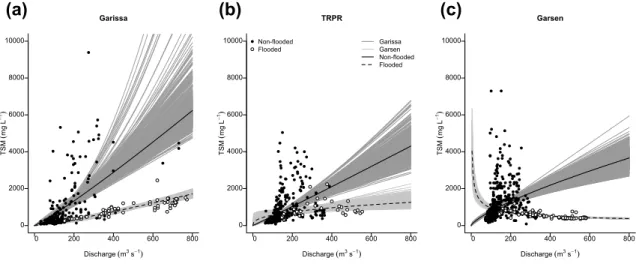
whereby a distinction was made between non-flooded and flooded conditions, according to the previously discussed thresholds. Suspended sediment transport was related to dis-charge through a power function, TSM = a × Qb, whereby
TSM denotes the suspended sediment concentration in mg
L− 1, Q the discharge in m3 s− 1 while a and b are regression
coefficients (Fig. 3; Table 1). Daily sediment fluxes were obtained by multiplication of the daily concentration with the daily discharge, and summing over each year resulted in the annual sediment flux.
Data on concentrations of POC, DOC, and dissolved IC (DIC) were similarly combined from different datasets. Daily POC, DOC and DIC concentration data at Garissa and Garsen were obtained during three wet season cam-paigns in 2012 (n = 37 per site), 2013 (n = 52 per site) and 2014 (n = 45 per site) (Geeraert et al. 2017). The dataset of Garissa was further expanded with data from monthly (Tamooh et al. 2014) and biweekly (unpublished data) monitoring over the period January 2009 - December 2013 (nPOC = 85, nDOC = 68, nDIC = 86). The sampling protocols
(a)
(b)
(c)
Fig. 3 Non-linear least square regression curves of the TSM as a function of discharge for a Garissa, b TRPR and c Garsen differ-entiated according to the hydrological condition (flooded vs.
non-flooded). The grey background colours indicate the range of the regression curves from the 200 bootstrap simulations
Table 1 Non-linear regression coefficients for the equation TSM = a × Qb at the three sites under non-flooded and flooded
condi-tions
n is the number of observations
Site Condition a b R2 n Garissa Non-flooded 3.659 1.113 0.35 246 Flooded 0.595 1.192 0.75 77 TRPR Non-flooded 4.408 1.030 0.24 566 Flooded 95.683 0.385 0.15 40 Garsen Non-flooded 25.297 0.744 0.12 676 Flooded 7551.566 -0.450 0.58 100
used to obtain concentrations of POC, DOC and DIC have been presented in Geeraert et al. (2017) for the wet season campaigns, and in Tamooh et al. (2014) for the biweekly and monthly samples of DIC, as an empirical relationship with total alkalinity (TA) was used to calculate the DIC concen-tration instead of the calculation based on TA and pCO2.
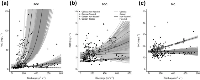
The annual fluxes of POC and DOC were calculated in R based on nonlinear least-squares regression equations between the untransformed C concentration and the dis-charge (Fig. 4). The regression coefficients for POC and DOC were calculated for the equation C = a × Qb whereby
C denotes the C concentration in mg L− 1. Due to the
absence of a convergent solution for the non-flooded con-centrations of DIC, the DIC concentration was estimated based on a single linear regression curve (C = aQ + b) at each site, including both the non-flooded and flooded observations. A maximum POC concentration of 125 mg L− 1 was set for both sites to avoid an unrealistic
overesti-mation during non-flooded conditions. Daily C concen-trations were multiplied with daily discharge and the sum per year was made for each of the C species.
The uncertainty in the regression curves of TSM and the C species was simulated by a bootstrap method. By using the package ‘Boot’ in R (version 1.3–18), a subset of the original dataset was constructed by randomly omit-ting certain observations and selecomit-ting other observations multiple times in such a way that the initial number of observations is maintained. Regression coefficients were calculated for 200 of those subsets. A maximum limit was set for the daily concentrations of POC (125 mg L− 1) and
TSM (1000 mg L− 1), as some regression lines resulted in
unrealistically high values at high, but not yet flooded, discharge conditions. Subsequently, the annual fluxes were calculated from the daily concentrations from each regression line, or by a combination of regression lines
for the species where the distinction between flooded and non-flooded conditions was made. The ranges of the flux difference and percentage contribution obtained through this bootstrap method are graphically presented by the grey–shaded areas in Figs. 3, 4, 7 and 8.
Analysis of seasonal variation
To examine seasonal patterns in sediment and C fluxes, we focus on the years 2012 and 2013 since this period has the most dense data availability for TSM, POC, DOC and DIC, and the gaps in the daily discharge dataset during this period (135 days in Garissa, 9 days in Garsen) occurred mainly dur-ing dry conditions, where data filldur-ing is relatively straight-forward and does not substantially influence the annual flux estimates. The delineation of the season was done by fixed dates in order to have the same number of days per season for each year. The long wet season ran from April 1st until June 15th (n = 76 days), while the short wet season ran from October 15th until December 31st (n = 78 days). Together, the two remaining periods of the year formed the dry season (n = 212 days in 2012 and 211 days in 2013).
Analysis of different hydrological conditions
The expected changes in the hydrology were assessed by constructing different discharge series under four differ-ent scenarios: (1) an overall increase of 10%, (2) an overall decrease of 10%, (3) 10% increase during the wet seasons and 10% decrease during the dry season, (4) 10% increase during the wet season and no change during the dry season. These changes were applied to the 73 years of discharge measurements. The dry seasons occurred from January to March and from mid-July to the end of September, while the wet seasons lasted from April to mid-July and from October
(a)
(b)
(c)
Fig. 4 Regression curves for a POC, b DOC and c DIC, whereby a distinction is made for non-flooded and flooded conditions for POC and DOC. The grey background colours indicate the range of the regression curves from the 200 bootstrap simulations
to December. A linear regression was made between the dif-ferent seasons to obtain smooth changes. The flooded days and fluxes were calculated as explained in Sects. “Study area” and “Fluxes of sediment and carbon” by using the regression coefficients for the whole dataset without boot-strap method. A loess smoothing function with a span of 0.4 (package ggplot2 2.2.1 in R 3.4.0) was applied in the plots to improve the visual distinction between the different scenarios.
Analysis of sampling frequency
To assess the influence of the sampling frequency on the annual TSM flux, we used the TSM measurements of Garsen. A total of 644 samples was collected at this site over 657 days (May 2012–March 2014), of which 55 sam-ples were taken under flooded conditions: the latter were all taken in 2013 as no flooding occurred in 2012. Subsets of the total dataset were taken at regular intervals at a frequency of 1, 2, 3, 4, 7, 14, 21 and 30 days. Up to four different starting dates were chosen per interval in order to assess the variability within a certain sampling interval, resulting in a total of 26 subsets.
Three regression curves were fit to each subset: one with all data included and two where the distinction was
made between flooded and non-flooded conditions accord-ing to the previously discussed criteria. The scenario with all data included simulates the situation where there is no prior knowledge about the existence of different hydrologi-cal conditions. No distinction according to conditions was made for a sampling frequency of 30 days and for one sub-set of 21 days because there were insufficient observations during flooded conditions. Subsequently, the annual fluxes were calculated for 2012 and 2013 by applying the regres-sion curves to the daily water discharge measurements and summing the daily sediment fluxes.
Results
Seasonal variations
The total dry season discharge was constant, both spatially (Garissa vs. Garsen) and temporally (2012 vs. 2013), with values of 1.9 and 2.1 km3 in Garissa and 1.9 and 2.0 km3
in Garsen, in 2012 and 2013 respectively (Fig. 5a). The dry seasons still accounted for at least one-third of the total annual discharge (34–44%), which is smaller than their proportion in time (~ 58% of the year). The varia-tions between the water fluxes of the wet seasons were
(a)
(b)
(c)
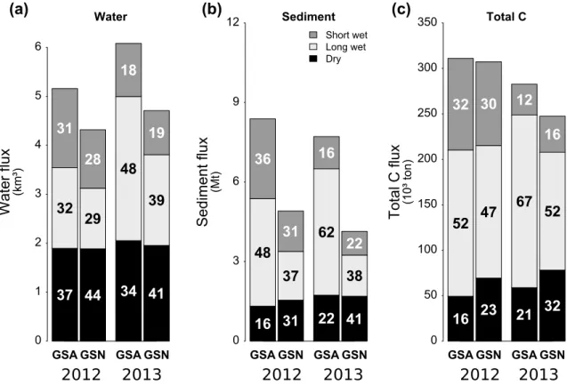
Fig. 5 Flux of a water, b sediment and c total C in 2012 and 2013 according to the seasons at Garissa (GSA) and Garsen (GSN). The numbers are the percentage share of each season in the annual flux
the main source of variation in annual discharge and of variation between the two sites. During each wet season, we observed a significant downstream decrease in dis-charge of ca. 25% in both seasons of 2012, and of 37 and 17% during the long and short wet seasons of 2013. This decrease is caused by infiltration in the river bed and/or floodplain, evaporation and the absence of considerable tributaries. The two wet seasons of 2012 had a comparable relative contribution to the annual water flux at each site (28–32%), while in 2013 the flooded long wet season prised a significantly larger share (48 and 39%) in com-parison to the suppressed short wet season (18 and 19%). The dry seasons had a lower relative contribution in the annual flux of the sediment and total carbon (TC) than they had in the water flux (Fig. 5b, c). Furthermore, a clear downstream increase of the TC flux was observed during the dry season. The downstream increase in TC during the dry seasons in 2012 and 2013 was less than the decrease observed during the wet seasons, leading to a net down-stream decrease in TC over the whole year. The relative contribution of the dry season to the total annual fluxes of water, sediment and C was always greater downstream in Garsen than it was upstream in Garissa, which illustrates that the floodplain downstream of Garissa acted as a buffer
during the high flows by reducing and/or delaying fluxes. The large differences in the relative seasonal contribu-tion of the water, sediment and C fluxes indicated that the daily averaged concentration of TSM and C varies strongly between the seasons (Fig. 5).
POC was found to be the dominant C pool on both the annual scale and during the wet seasons (Fig. 6). During the dry season, the POC and DIC fluxes were similar in magni-tude. The POC flux strongly increased downstream during the dry season and to a lesser extent during the short wet sea-son of 2013, while during the long wet seasea-sons, a decrease was observed. The DOC flux during the dry seasons was constant in space and time. During the non-flooded wet sea-sons, there was a slight downstream decrease in DOC flux, while there was no change during the flooded wet season in 2013. The DIC flux increased slightly during the dry season, while there was a limited decrease during all wet seasons.
Differences in longitudinal fluxes
The difference between the incoming flux at Garissa and the outgoing flux at Garsen determines whether the river stretch was either a retention area or a source area for the sediment or C with respect to the various riverine pools.
Fig. 6 Distribution of riverine
C species at Garissa (GSA) and Garsen (GSN) in 2012 and 2013 for the a whole year, b dry season, c long wet season, d short wet season. The numbers represent the absolute values of the fluxes in 103 t
(a)
(b)
While we use the term retention when the downstream flux was smaller than the upstream flux (FGarissa − FGarsen > 0),
it does not imply anything about the fate of the retained C, which can either be stored in the river or floodplain or can be further processed (including outgassing to the atmosphere in the case of DIC). The flux differences (Garissa–Garsen) were calculated for random combinations of the 200 annual fluxes per year at each site and were plotted as a function of the total annual discharge at Garissa (Fig. 7, left graphs). Similarly, the difference in fluxes was also expressed as a
percentage of the upstream flux at Garissa (Fig. 7, right panels).
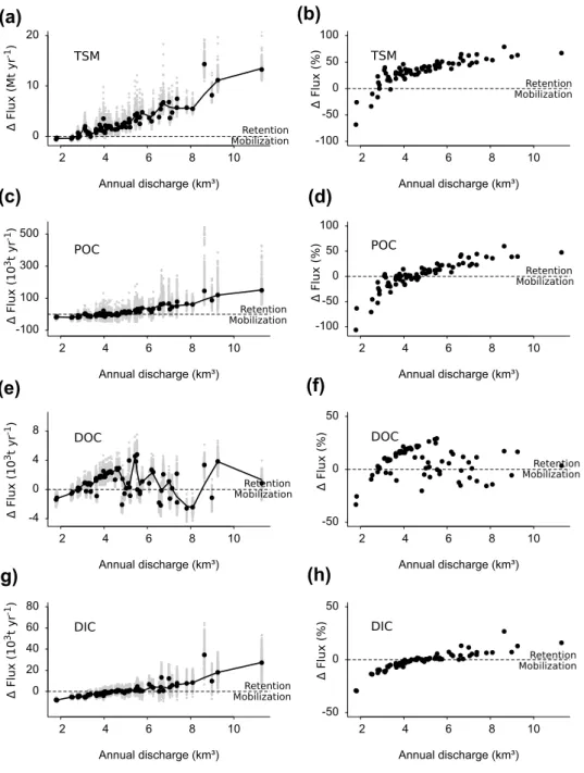
Retention of sediment occurred under all annual water fluxes, except where the water flux was < 3 km3 year− 1.
Fur-thermore, a larger annual water flux led to a larger absolute deposition of sediment (Fig. 7a). The POC flux difference exhibited a slightly different pattern: below a water flux of ca. 3.5 km3 year− 1 there was usually a net downstream
increase in C flux, between 3.5 and 6 km3 year− 1 the C fluxes
were balanced, while above 6 km3 year− 1 a general retention
Fig. 7 Retention (positive) or mobilization (negative) based on the difference in fluxes (GSA-GSN) in absolute (left graphs) and relative (right graphs) values of a, b TSM, c,
d POC, e, f DOC and g, h DIC
between Garissa (GSA) and Garsen (GSN) as a function of the annual discharge at Garissa. The trendline is a LOWESS smoothing with the default parameter values in the stats package in R
(a)
(b)
(c)
(d)
(e)
(f)
of POC was estimated (Fig. 7c). Both for TSM and POC, the relative change ranged between − 106 and 78%. The pattern of DOC was less consistent (Fig. 7e, f). Initially, there was an increase in DOC flux difference between the sites with increasing discharge. However, once more days with flooded conditions were occurring, there was considerable scatter, whereby the negative differences (net export over the river stretch considered) occurred in years with a high number (> 100) of flooded days. The relative change in DOC fluxes (− 33 to 29%) had a smaller range than for POC. Finally, the DIC fluxes indicated a larger downstream DIC flux than the upstream DIC flux at an annual discharge below ~ 5 km3
year− 1, while at higher discharge, the upstream DIC flux
became larger (Fig. 7g-h). This is contrasting to what might be expected from the rating curves, but can be explained by the large downstream decrease in water discharge. As was the case for DOC, the relative change in DIC fluxes was limited (− 29 to 27%).
The cumulative effect over all the annual net differences over the whole historical observation period resulted in a net average annual sediment deposition rate of ~ 2.9 Mt year− 1.
This deposition implies that a large amount of unconsoli-dated sediment is available for autogenic processes to keep the sediment concentration near transport capacity (Geer-aert et al. 2015). The long-term balance of the C species also suggests a net retention of C within the river stretch for POC, DOC and DIC, with an average annual amount of ~ 18,000, ~ 920 and ~ 1200 tC year−1, respectively. Although
these measurements give no indication to the fate of the retained C, part of the POC will likely be deposited in the floodplain while some will be respired, while the excess DIC is expected to have evaded to the atmosphere, as has been quantified for distinct wet seasons in the Tana River (Geer-aert et al. 2017).
Carbon species differentiation as a function of discharge
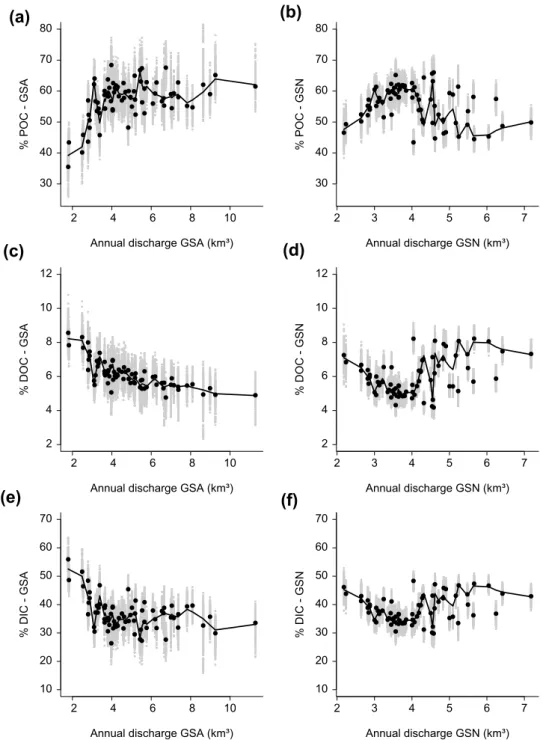
The relative contribution of each C species in the TC flux was also correlated with the annual water flux (Fig. 8). The contribution of POC in Garissa was relatively low (~ 30–40%) during dry years, but increased notably with increasing annual discharge and became stable around 60–70%. At Garsen, the contribution of POC was also relatively low at low discharge, but higher than in Garissa (~ 40–50%). At annual discharges between 3 and 4 km3, 60%
of the TC in Garsen was accounted for by POC, while it was very variable at higher annual discharge. Both dissolved fractions showed the opposite pattern: the contribution of DOC in Garissa decreased from ca. 9–5%, while in Garsen it decreased initially between 8% and 4%, and became scat-tered at high annual water fluxes. The DIC was the most
important C species at an annual discharge below 3 km3
year− 1 at Garissa and below 2.75 km3 year− 1at Garsen, but
then decreased significantly. The scatter which was observed at high discharge in Garsen was related to the occurrence of flooded conditions, whereby the years with a high number of flooded days had a higher contribution of DIC and DOC.
Hydrological scenarios
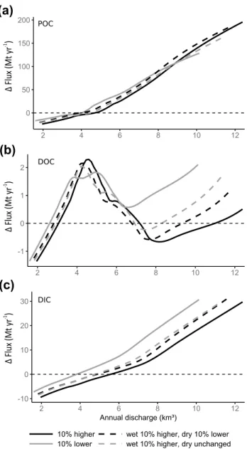
The different hydrological scenarios show non-linear behav-iour (Fig. 9): while the retention of all the C species is gen-erally larger when the daily discharge is reduced, this is no longer the case for POC at very high annual discharge and for DOC at a medium discharge range. This can be explained by the fewer days under flooded conditions for which the rating curve with low concentrations at high discharge is required during the dryer scenario.
Comparison of the scenarios with 10% increase in dis-charge during the wet season, but wetter, dryer or similar discharge during the dry season reveals different behaviour of the different C species. POC retention at intermediate discharge is lowest when both seasons got wetter, while at high discharge retention of POC will increase when the dry seasons will become both wetter or dryer compared to the current situation. The DOC retention shows the largest varia-tion at high discharge because years with many flooded days had often a net mobilisation of DOC (Fig. 7). The DIC is hardly influenced by a decrease in discharge during the dry season, but an increase during the dry season lowered the amount of DIC retention significantly.
The long-term balance of the different scenarios shows an overall retention of all C species (Table 2). The highest POC retention occurred in the scenario with increased wet season discharge and decreased dry season discharge. Both dissolved fluxes retained most C when the discharge was 10% lower throughout the year, while a general increase in discharge led to less retention.
Discussion
Sampling frequency and timing
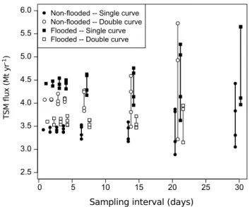
The applied methodology relied strongly on the differentia-tion between the two hydrological condidifferentia-tions: flooded vs. non-flooded rating curves. The high-frequency sampling of the sediment allowed us to assess what errors would be made if we failed to identify the two conditions or failed to have enough observations of each of the conditions. Two major observations can be drawn from the analysis for a year with-out (2012) and with flooding (2013) (Fig. 10). Firstly, the large scatter in annual flux estimates at lower sampling fre-quencies indicates that when the sampling interval is above
ca. 10 days, total annual fluxes could not be estimated with a high precision. Secondly, calculated fluxes differ considera-bly if the different rating curves for flooded and non-flooded conditions were used (double curve) or not (single curve). In 2012, when no flooded conditions were observed, the annual flux was lower when all sampling points (including flooded points in the dataset) were used for the construction of the rating curves. The opposite was true for the year 2013 when flooding occurred. This clearly shows that the identification
of different regimes is important in order to correctly esti-mate annual fluxes (Fig. 10).
When the sampling became less frequent, the number of samples taken under flooded conditions decreased rapidly and became very small when the sampling interval exceeded 7 days (Table 3). It may therefore be worthwhile to increase the sampling frequency during the wet seasons, in order to be able to identify different regimes. Similar results were obtained in a small stream where additional measurements
Fig. 8 Percentage contribution of a, b POC, c, d DOC and e,
f DIC in the total C flux as a
function of the annual water flux in Garissa (left panels) and Garsen (right panels). The trendline is a LOWESS smooth-ing with the default parameter values in the stats package in R
(a)
(b)
(c)
(d)
during high discharge events increased the accuracy of the DOC load significantly (Büttner and Tittel 2013).
The results of the annual C flux calculations showed that the hydrological characteristics of the wet seasons in a spe-cific year formed the dominant factor for the sediment and C flux estimates in that year. Years with a similar total annual discharge may still show important differences in sediment and C flux, as the discharge in 1 year can be well distributed over small peaks and not lead to significant flooding or a period of significant floods in combination with a prolonged period of low discharges may be experienced. This again illustrates that, for river systems with a high day-to-day vari-ation in discharge, very high frequency measurements (e.g. daily) are a requirement for an accurate calculation of annual fluxes.
Despite the uncertainty related to the inter-annual vari-ability, our annual flux estimates showed clear tendencies as a function of annual discharge. As more data are collected, these trends can be further refined. In addition, the sampling effort can be made more efficient through the identification of the different hydrological regimes and the adaptation of the sampling frequency to the characteristics of the regime. Finally, a perfect rating curve is not possible because there will always be a considerable amount of scatter associated with the natural variability of the concentrations.
Influence of flood season length
In this river system, the identification of the two different hydrological regimes during the wet season was important to calculate the annual fluxes. To recognise other river systems where this distinction is important, we made some simple calculations to identify the importance of the length of the wet/flooded season, the difference in concentration between the wet season without flooding and with flooding and the magnitude of the discharge during the wet season.
In those calculations, a very simple hydrological year was constructed, where only two discharges occurred: low discharge (dry season) and high discharge (wet season). The timing of the high discharge was not important because the daily concentration was calculated based on the daily dis-charge and independent from the other days. Therefore, vari-ations in the length of the flooding season were simulated by varying the number of high discharge days in the year between 0 and 20% days with increments of 1%.
(a)
(b)
(c)
Fig. 9 Retention (positive) or mobilization (negative) of a POC, b
DOC and c DIC based on the difference in fluxes between Garissa and Garsen as a function of the annual discharge at Garissa for four different discharge scenarios. The trendline is a loess smoothing with a span of 0.6 in the ggplot package in R
Table 2 Annual average of the difference in C fluxes between Garissa (upstream) and Garsen (downstream) over 73 years of discharge measurements for the original discharge values and four different scenarios
POC (tC year− 1) DOC (tC year− 1) DIC (tC year− 1)
Original discharge ~ 18,000 ~ 920 ~ 1200
All 10% higher 22,394 756 261
All 10% lower 15,172 1024 2470
Wet 10% higher, dry 10% lower 24,454 773 1241
Subsequently we calculated for each of these hydrologi-cal years, with varying length of wet season, the annual constituent flux of (1) a river with one discharge regime, which was characterized by low concentrations during low
discharge and high concentrations during high discharge and (2) a river with two discharge regimes, which had low concentrations during low discharge and also low concen-trations during high discharge (Table 4). The annual fluxes were compared by taking the ratio of the double discharge regime over the single discharge regime. The concentration and the discharge were varied in different scenarios to see how much effect each of them has on the annual flux under the two discharge regimes.
The first observation drawn from these calculations was that the difference between the two situations (single dis-charge vs. double disdis-charge regime) converged to a specific value (Fig. 11). That value was depending on the difference between the concentration during the wet season. Even in a year with only 1% flooded days (= 3.65 days), there was already a flux difference of 13% between the two situations at the intermediate parameters. The magnitude of the dis-charge determined how fast the difference converged towards the percentage determined by the concentration difference. For example, there was a 17% reduction in flux with 1% flooded days in the situation of 700 m³ s− 1, while this was
only 8% when the discharge was only 300 m³ s− 1 during
those 3.65 days. So, rivers with large differences in concen-trations at high discharge will be most prone to errors due to missing out on concentration measurements during high discharge and thereby missing out on variations in the hydro-logical regime. Special efforts to capture that variation and preferably to find a systematic pattern will increase the reli-ability of the flux measurements, because even by missing
Fig. 10 Effect of the sampling frequency and the identification of dif-ferent hydrological conditions on the sediment flux calculations in Garsen in 2012 (non-flooded) and 2013 (flooded). Different regres-sion equations for flooded and non-flooded conditions were applied in the ‘Double curve’ fluxes. The range per sampling interval was obtained by choosing up to four different starting dates for the time series. For each sampling interval, the estimated fluxes were slightly shifted along the x axis to improve visibility
Fig. 11 Ratio between the annual flux of a river with two discharge regimes and a river with one discharge regime over a varying length of
flooded season and for a different concentrations during the single discharge regime or b different discharges during the flooded conditions
Table 3 Number of
observations (± 1, depending on the starting date) that were used in the construction of the rating curves for different sampling frequencies
Sampling interval
1 day 2 days 3 days 4 days 7 days 14 days 21 days 30 days
n—all 644 322 215 161 92 46 31 22
n—non-flooded 589 594 196 147 85 42 28 20
reduced concentrations during only 4 days, an annual over-estimate of 10% can easily be obtained.
Comparison with other measurements
Previous annual flux estimates for the Tana River by Tamooh et al. (2014) were based on monthly samplings from 2009 to 2011 at Garissa (n = 39) and TRPR (n = 40), the latter located ca. 80 km upstream of Garsen (measured along the river). The annual fluxes were calculated using two software applications which use different calculation methods. GUMLEAF calculated discharge weighted aver-age concentrations, while LOADEST fitted a regression line based on the (Adjusted) Maximum Likelihood Estima-tion (Tamooh et al. 2014).
The annual fluxes of TSM over the period 2009–2011 at Garissa and TRPR were very comparable between the three methods (Table 5). This good agreement is explained by the occurrence of only one hydrological regime over the period 2009–2011. This is equivalent with the non-flooded regression line in the method presented here. If the method of Tamooh et al. (2014) would have been used with the same input data in a period with flooding, there would have been a large overestimation of the flux, com-parable to the situation ‘flooded-single curve’ in Fig. 10. Estimated annual fluxes of sediment and C in TRPR are much lower in comparison to the up- and downstream sites of Garissa and Garsen, except for DIC. This is potentially due to the methodology of the discharge calculation at TRPR used by Tamooh et al. (2014), whereby the very high discharges were suppressed, leading to much lower discharge in TRPR compared to Garsen. However, even in our calculations, whereby the discharge in TRPR is cal-culated as a distance-weighted average of the discharge in Garissa and Garsen, the annual TSM flux in TRPR is less than the flux in Garissa and Garsen. This can be explained by significant deposition of sediment between Garissa and TRPR and a subsequent mobilization of sediment between TRPR and Garsen. An alternative and more likely expla-nation is that the discharge at TRPR is underestimated by the distance-weighted average method, and as a result the
TSM flux is also underestimated. Downstream of TRPR, the river shifts from a meandering river pattern to a more anastomosing pattern. The water loss is likely to be larger in the anastomosing part of the river and therefore the linear interpolation of discharge loss will lead to an under-estimation of the discharges in TRPR. The comparison of the average fluxes over the 3 year period with the average fluxes over the longer time frame indicates that 2009–2011 was a period with relatively low fluxes.
Table 4 Overview of the parameters in the calculations between a river with one hydrological regime and one with two hydrological regimes
Only one parameter (concentration, C or discharge, Q) was varied at the same time, while the intermediate value was used when that parameter was not varied
C (g L− 1) Q (m3 s− 1)
No flooding 1 100
Flooding—1 regime 2–4–6 300–500–700
Flooding—2 regimes 1 300–500–700
Table 5 Comparison of the annual fluxes and specific yield at Garissa (GSA), Tana River Primate Reserve (TRPR) and Garsen (GSN) between the estimates by Tamooh et al. (2014) with only monthly measurements over the period 2009–2011 and the results based on all available measurements over the same period and over a longer term (1942–2014) without applying a bootstrap method
Gumleaf
2009–2011 Loadest2009–2011 This study2009–2011 This study1942–2014 Annual fluxes (TSM: Mt year− 1, C: 103 t year− 1)
TSM GSA 5.9 8.7 5.2 6.6 TRPR 3.2 3.1 2.9 GSN 3.5 3.8 POC GSA 92.5 104.9 97.7 118.1 TRPR 39.6 36.6 GSN 109.9 113.3 DOC GSA 9.6 10.0 10.2 11.8 TRPR 6.0 6.5 GSN 8.8 11.2 DIC GSA 57.6 63.6 59.3 74.6 TRPR 56.4 62.2 GSN 61.2 73.4
Annual specific yield (t km− 2 year− 1)
TSM GSA 169.4 247.7 161.3 203.3 TRPR 48.12 46.4 44.1 GSN 42.9 46.0 POC GSA 2.64 3.00 3.01 3.6 TRPR 0.59 0.55 GSN 1.35 1.4 DOC GSA 0.27 0.28 0.31 0.4 TRPR 0.09 0.10 GSN 0.11 0.1 DIC GSA 1.64 1.82 1.83 2.3 TRPR 0.84 0.94 GSN 0.75 0.9
Comparisons between catchments are usually made based on the specific yields (SY), which is the flux normal-ized to the upstream catchment area (32,500, 66,500 and 81,700 km2 for the Tana River in Garissa, TRPR and Garsen
respectively) (Table 5). The SY in Garissa is roughly three-fold the SY in Garsen. This can be explained by the very large catchment area between Garissa and Garsen which rarely delivers sediment to the river due to the semi-arid conditions.
The specific sediment yield of African catchments ranges between 0.2 and 15,700 t km2 year− 1 with median and
aver-age values of 160 and 634 t km2 year− 1, respectively
(Van-maercke et al. 2014). The values for the Tana River (203.3 and 46.0 t km2 year− 1 for Garissa and Garsen respectively)
are well within this range, although on the lower side. Sedi-ment yields decrease with increasing catchSedi-ment area, and applying the regression equation between SY and catch-ment area developed by Vanmaercke et al. (2014) to our sites resulted in a predicted specific sediment yield of 79.2 and 68.3 t km2 year− 1 for Garissa and Garsen respectively.
Considering the generalisations and assumptions, those pre-dictions are fairly well in line with our measurements, with a gross underestimation for Garissa (203.3 t km2 year− 1)
and a small overestimation for Garsen (46.0 t km2 year− 1)
in respect to our calculations.
Comparing the C yields of the Tana River with other river systems indicated a relatively high POC yield in the Tana River and in general a limited yield of dissolved C; A global dataset on SY for organic C indicates that the SY of POC ranged between 0.002 and 92.5 t km2 year− 1, and between
0.001 and 56.9 t km2 yearyear− 1 for DOC (Alvarez-Cobelas
et al. 2012), which are very broad ranges which encapsulate our observations. The tropical rivers dataset compiled by Huang et al. (2012) calculated average yields for POC, DOC and DIC of 0.33, 1.00 and 0.63 t km2 year− 1, respectively,
for tropical Africa, and 2.05, 2.13 and 3.29 t km2 year− 1,
respectively, for the tropics in total.
Implications of environmental changes
The dependency of retention/mobilization on the total annual discharge implies that changes in the hydrological regime are expected to have a significant influence on both the sedi-ment and C fluxes in the river, irrespective of whether those changes are due to climate change or human impact in the catchment. Projections for the precipitation in the area of the Tana River show a small tendency for increased pre-cipitation (IPCC 2013). This would result in higher annual discharge fluxes which lead to enhanced storage of sediment and retention of POC between both sites at high annual dis-charge, while the DIC retention decreases (Fig. 9; Table 2). Besides the annual change in discharge, climate change is also expected to affect the seasonal distribution of the
discharge (Shongwe et al. 2011). Increased extreme precipi-tation events during the wet season are expected to result in more flooded seasons, which leads to a slight reduction of the retention of all the species (Table 2). For the dissolved species, this is likely caused by an increased input from the inundated floodplain. More or longer drought periods will increase the time that mobilisation of sediment and C can take place, which especially has an effect on the POC flux in the river (Fig. 6; Table 2).
The human impact due to the construction of the High Grand Falls dam is expected to act at two different levels: the sediment supply and the seasonal water distribution (Tana and Athi Rivers Development Authority 2016). Ear-lier analyses of the sediment fluxes at Garissa have shown that floodplain processes were able to buffer the sediment losses caused by the dams (Geeraert et al. 2015). If, after construction of the HGF dam, the sediment load of the river would not be at transport capacity anymore when it reaches Garissa, it can be expected that the degree of retention between Garissa and Garsen will decrease and the trendlines in Fig. 7 will shift down as sediment is mobilized from the floodplain. Besides trapping of the sediment, biogeochemi-cal processes in the reservoir can alter the nutrient fluxes in the downstream river (Van Cappellen and Maavara 2016; Maavara et al. 2017), but their effects will be beyond what can be derived from our rating curves.
The seasonal change in water discharge following the construction of the present cascade of dams can be sum-marized as a decrease of the discharge during the long wet season and an increase in discharge during the dry seasons (Maingi and Marsh 2002). If this pattern were enhanced after the construction of the HGF dam, then a larger fraction of the annual water flux would occur during the dry season. This is likely to result in a decrease of retention of sediment and C between both sites, as the dry-season flux of TSM and total C is larger in Garsen than in Garissa (Fig. 5). The filling of the reservoir will also reduce the downstream water flux during the initial years as the volume of the reservoir (5.7 km3) is of the same order of magnitude as the measured
total annual water flux in either 2012 or 2013 (Fig. 5). Even after the filling of the dam, annual discharge is expected to decrease due to abstraction of water for irrigation purposes and also increased evaporation. In both situations, the man-agement decisions with respect to the timing and magni-tude of the water release will affect the downstream C flux. These changes in flux due to the hydrological alterations will interact with biogeochemical processes which occur in the reservoir.
Conclusions
Large tropical river systems can transport large amounts of sediment and C, but those fluxes can change due to alterna-tions in the hydrological condialterna-tions due to climate change or dam construction. To assess the potential changes in the sediment and C flux in the lower Tana River, we first investigated the seasonal differences in fluxes between a year without flooding and a year with considerable over-bank flooding. The differences in annual fluxes are mainly determined by the characteristics of the wet season hydro-graph, while the magnitude of the dry season fluxes is fairly constant. The sediment fluxes decreased strongly between Garissa and Garsen during the short wet and long wet seasons, while the annual TC flux showed only a slight decrease in the downstream direction. POC was the domi-nant C species over the whole year, but the DIC flux was slightly larger than the POC flux during some dry seasons. The DOC flux was always the smallest contributor to the TC flux and showed limited spatial and temporal variation.
The differentiation between the non-flooded and flooded conditions was important for the extrapolation, because otherwise large errors were introduced: when both condi-tions are present in the sample database, the annual TSM flux of non-flooded years was underestimated when the differentiation between the regimes was not made, while the flux of flooded years was overestimated. Increas-ing the samplIncreas-ing frequency when shifts in the discharge regime are expected will therefore improve the annual flux estimates.
Applying the present-day relationships between dis-charge and concentration on a long term disdis-charge dataset revealed that at lower annual discharge, there was on aver-age a downstream increase in sediment and C fluxes, while retention between both sites was expected at higher annual discharge values. The integrated signal over the hydro-logical range was a net retention of TSM, POC, DOC as well as DIC. The relative fractions of the C species varied also as a function of the annual discharge. The DIC was the dominant C species at low annual discharge, while the POC dominated at high annual discharge. The relative importance of DOC was always below 10% and decreased as the annual discharge increased.
An overall increase in discharge would lead to increased POC retention and a decrease of dissolved C retention. The response of the different C species to seasonal variations is much more variable. The effect of the High Grand Falls dam will depend on management decisions concerning the regulation of the outlet discharge, but if discharges during the dry seasons are increased, this may lead to less reten-tion of sediment and C on the floodplain.
Acknowledgements Funding was provided by the KU Leuven Special Research Fund, the Research Foundation Flanders (FWO–Vlaanderen, project G024012N), and an ERC Starting Grant (240002, AFRIVAL). We are grateful to the Kenya Wildlife Service (KWS) for assistance during field experiments and to the Water Resources Management Authority (WRMA) for assistance during the ADCP measurements and for sharing discharge data. AVB is a senior research associate at the FRS-FNRS
Author contributions S. Bouillon, N. Geeraert, T. Marwick, F.O. Omengo and F. Tamooh were involved in the data collection. N. Geer-aert prepared the manuscript with contributions from all co-authors. Compliance with ethical standards
Conflict of interest The authors declare that they have no conflict of interest.
References
Abril G, Martinez J-M, Artigas LF, Moreira-Turcq P, Benedetti MF, Vidal L, Meziane T, Kim J-H, Bernardes MC, Savoye N, Deborde J, Souza EL, Albéric P, Souza MFL de, Roland F (2014) Ama-zon River carbon dioxide outgassing fuelled by wetlands. Nature 505:395–398. https ://doi.org/10.1038/natur e1279 7
Aitkenhead J, McDowell W (2000) Soil C:N ratio as a predictor of annual riverine DOC flux at local and global scales. Global Bio-geochem Cycles 14:127–138
Aldrian E, Chen C-TA, Adi S, Sudiana N, Nugroho SP (2008) Spatial and seasonal dynamics of riverine carbon fluxes of the Brantas catchment in East Java. J Geophys Res 113 (G3). https ://doi. org/10.1029/2007J G0006 26
Alvarez-Cobelas M, Angeler D, Sánchez-Carillo S, Almendros G (2012) A worldwide view of organic carbon export from catch-ments. Biogeochemistry 107:275–293. https ://doi.org/10.1007/ s1053 3-010-9553-z
Beusen AHW, Dekkers ALM, Bouwman AF, Ludwig W, Harrison J (2005) Estimation of global river transport of sediments and associated particulate C, N, and P. Global Biogeochem Cycles 19:GB4S05. https ://doi.org/10.1029/2005G B0024 53
Bird M, Robinson R, Win Oo N, Maung Aye M, Lu X, Higgitt D, Swe A, Tun T, Lhaing Win S, Sandar Aye K, Mi Mi Win K, Hoey T (2008) A preliminary estimate of organic carbon transport by the Ayeyarwady (Irrawaddy) and Thanlwin (Salween) Rivers of Myanmar. Quat Int 186:113–122
Borges AV, Darchambeau F, Teodoru CR, Marwick TR, Tamooh F, Geeraert N, Omengo FO, Guérin F, Lambert T, Morana C, Okuku E, Bouillon S (2015) Globally significant greenhouse-gas emis-sions from African inland waters. Nat Geosci 8:637–642. https :// doi.org/10.1038/ngeo2 486
Bouillon S, Abril G, Borges AV, Dehairs F, Govers G, Hughes HJ, Merckx R, Meysman FJR (2009) Distribution, origin and cycling of carbon in the Tana River (Kenya): a dry season basin-scale survey from headwaters to the delta. Biogeosciences 6:2475–2493 Bouillon S, Yambélé A, Spencer RGM, Gillikin DP, Hernes PJ, Six J, Merckx R, Borges AV (2012) Organic matter sources, fluxes and greenhouse gas exchange in the Oubangui River (Congo River basin). Biogeosciences 9:2045–2062. https ://doi.org/10.5194/ bg-9-2045-2012
Brunet F, Dubois K, Veizer J, Ndondo GN, Ngoupayou JN, Boeg-lin J-L, Probst J-L (2009) Terrestrial and fluvial carbon fluxes
in a tropical watershed: Nyong basin, Cameroon. Chem Geol 265:563–572
Büttner O, Tittel J (2013) Uncertainties in dissolved organic carbon load estimation in a small stream. J Hydrol Hydromech 61:81–83. https ://doi.org/10.2478/johh-2013-0010
Coynel A, Seyler P, Etcheber H, Meybeck M, Orange D (2005) Spatial and seasonal dynamics of total suspended sediment and organic carbon species in the Congo River. Global Biogeochem Cycles 19:GB4019. https ://doi.org/10.1029/2004G B0023 35
Degens E, Kempe S, Herrera R, Soliman H, Weibin G (1982) Transport of carbon and minerals in major world rivers, Part 1. Im Selbst-verlag des Geologisch-Paläontologischen Institutes der Universität Hamburg, SCOPE/UNEP Sonderbd, vol 52. p 766
Degens ET, Kempe S, Richey JE (1991) Biogeochemistry of major world rivers. Scope 42, Wiley, New York, pp 323–44
Depetris PJ, Kempe S (1993) Carbon dynamics and sources in the Parana River. Limnol Oceanogr 38:382–395
Garrels RM, Mackenzie FM (1971) Evolution of sedimentary rocks. WW Norton & Co., New York
Geeraert N, Omengo FO, Tamooh F, Paron P, Bouillon S, Govers G (2015) Sediment yield of the lower Tana River, Kenya, is insen-sitive to dam construction: sediment mobilization processes in a semi-arid tropical river system. Earth Surf Proc Land 40:1827– 1838. https ://doi.org/10.1002/esp.3763
Geeraert N, Omengo FO, Borges AV, Govers G, Bouillon S (2017) Shifts in the carbon dynamics in a tropical lowland river sys-tem (Tana River, Kenya) during flooded and non-flooded con-ditions. Biogeochemistry 1–23. https ://doi.org/10.1007/s1053 3-017-0292-2
Huang T-H, Fu Y-H, Pan P-Y, Chen C-TA (2012) Fluvial carbon fluxes in tropical rivers. Curr Opin Environ Sustain 4:162–169. https :// doi.org/10.1016/j.cosus t.2012.02.004
Indeje M, Semazzi FH, Ogallo LJ (2000) ENSO signals in East African rainfall seasons. Int J Climatol 20:19–46
IPCC (2013) Annex I: Atlas of Global and Regional Climate Projec-tions. In: Oldenborgh GJ van, Collins M, Arblaster J, Christensen JH, Marotzke J, Power SB, Zhou MM T (eds) Climate change 2013: The physical science basis. Contribution of working group I to the Fifth Assessment Report of the Intergovernmental Panel on Climate Change. Cambridge University Press, Cambridge Laraque A, Castellanos B, Steiger J, Lòpez JL, Pandi A, Rodriguez M,
Rosales J, Adèle G, Perez J, Lagane C (2013) A comparison of the suspended and dissolved matter dynamics of two large inter-tropical rivers draining into the Atlantic Ocean: the Congo and the Orinoco. Hydrol Process 27:2153–2170. https ://doi.org/10.1002/ hyp.9776
Lloret E, Dessert C, Gaillardet J, Albéric P, Crispi O, Chaduteau C, Benedetti MF (2011) Comparison of dissolved inorganic and organic carbon yields and fluxes in the watersheds of tropi-cal volcanic islands, examples from Guadeloupe (French West Indies). Chem Geol 280:65–78. https ://doi.org/10.1016/j.chemg eo.2010.10.016
Ludwig W, Probst J-L, Kempe S (1996) Predicting the oceanic input of organic carbon by continental erosion. Global Biogeochem Cycles 10:23–41
Ludwig W, Amiotte-Suchet P, Munhoven G, Probst J-L (1998) Atmos-pheric CO_2 consumption by continental erosion: present-day controls and implications for the last glacial maximum. Global Planet Change 16:107–120
Maavara T, Lauerwald R, Regnier P, Van Cappellen P (2017) Global perturbation of organic carbon cycling by river damming. Nat Commun 8:15347
Maingi JK, Marsh SE (2002) Quantifying hydrologic impacts following dam construction along the Tana River, Kenya. J Arid Environ 50:53–79. https ://doi.org/10.1006/jare.2000.0860
Mayorga E, Aufdenkampe AK, Masiello CA, Krusche AV, Hedges JI, Quay PD, Richey JE, Brown TA (2005) Young organic matter as a source of carbon dioxide outgassing from Amazonian rivers. Nature 436:538–541. https ://doi.org/10.1038/natur e0388 0 Mayorga E, Seitzinger SP, Harrison JA, Dumont E, Beusen AH,
Bouw-man A, Fekete BM, Kroeze C, Van Drecht G (2010) Global nutri-ent export from WaterSheds 2 (NEWS 2): model developmnutri-ent and implementation. Environ Model Softw 25:837–853
Meybeck M (1987) Global chemical weathering of surficial rocks esti-mated from river dissolved loads. Am J Sci 287:401–428 Mora A, Laraque A, Moreira-Turcq P, Alfonso JA (2014) Temporal
variation and fluxes of dissolved and particulate organic carbon in the Apure, Caura and Orinoco rivers, Venezuela. J S Am Earth Sci 54:47–56
Moreira-Turcq P, Seyler P, Guyot JL, Etcheber H (2003) Exportation of organic carbon from the Amazon River and its main tributaries. Hydrol Process 17:1329–1344
Moreira-Turcq P, Bonnet M-P, Amorim M, Bernardes M, Lagane C, Maurice L, Perez M, Seyler P (2013) Seasonal variability in con-centration, composition, age, and fluxes of particulate organic car-bon exchanged between the floodplain and Amazon River. Global Biogeochem Cycles 27:119–130
Richey J, Melack J, Aufdenkampe A, Ballester V, Hess L (2002) Out-gassing from Amazonian rivers and wetlands as a large tropical source of atmospheric CO2. Nature 416:617–620
Sarin M, Sudheer A, Balakrishna K (2002) Significance of riverine carbon transport: A case study of a large tropical river, Godavari (India). Sci China Ser C Life Sci 45:97–108
Schlesinger WH, Melack JM (1981) Transport of organic carbon in the world’s rivers. Tellus 33:172–187
Seitzinger SP, Harrison JA, Dumont E, Beusen AHW, Bouwman AF (2005) Sources and delivery of carbon, nitrogen, and phosphorus to the coastal zone: An overview of Global Nutrient Export from Watersheds (NEWS) models and their application. Global Biogeo-chem Cycles 19:GB4S01. https ://doi.org/10.1029/2005G B0026 06 Shongwe ME, Oldenborgh GJ van, Hurk van den B, Aalst van M (2011)
Projected changes in mean and extreme precipitation in Africa under global warming. Part II: East Africa. J Clim 24:3718–3733 Syvitski JPM, Cohen S, Kettner AJ, Brakenridge GR (2014) How
important and different are tropical rivers? An overview. Geomorphology 227:5–17. https ://doi.org/10.1016/j.geomo rph.2014.02.029
Tamooh F, Meersche Van den K, Meysman F, Marwick TR, Borges AV, Merckx R, Dehairs F, Schmidt S, Nyunja J, Bouillon S (2012) Dis-tribution and origin of suspended matter and organic carbon pools in the Tana River Basin, Kenya. Biogeosciences 9:2905–2920. https ://doi.org/10.5194/bg-9-2905-2012
Tamooh F, Borges AV, Meysman F, Meersche Van den K, Dehairs F, Merckx R, Bouillon S (2013) Dynamics of dissolved inor-ganic carbon and aquatic metabolism in the Tana River Basin, Kenya. Biogeosci Discuss 10:5175–5221. https ://doi.org/10.5194/ bgd-10-5175-2013
Tamooh F, Meysman FJR, Borges AV, Marwick TR, Meersche Van den K, Dehairs F, Merckx R, Bouillon S (2014) Sediment and car-bon fluxes along a longitudinal gradient in the lower Tana River (Kenya). J Geophys Res Biogeosci 119:1340–1353. https ://doi. org/10.1002/2013J G0023 58
Tana and Athi Rivers Development Authority (2016) Environmental and social impact assesment for the proposed High Grand Falls multi-purpose dam project. https ://www.nema.go.ke/image s/Docs/ EIA%20-%20106 0%20-%20106 9/EIA_1263%20Ken face%20for %20Tar da%20HGF %20dam %20rep ort.pdf
Van Cappellen P, Maavara T (2016) Rivers in the Anthropocene: global scale modifications of riverine nutrient fluxes by damming. Eco-hydrol Hydrobiol 16:106–111
Vanmaercke M, Poesen J, Broeckx J, Nyssen J (2014) Sediment yield in Africa. Earth Sci Rev 136:350–368. https ://doi.org/10.1016/j. earsc irev.2014.06.004
Wang ZA, Bienvenu DJ, Mann PJ, Hoering KA, Poulsen JR, Spencer RGM, Holmes RM (2013) Inorganic carbon speciation and fluxes in the Congo River. Geophys Res Lett 40:511–516. https ://doi. org/10.1002/grl.50160
Wiegner TN, Tubal RL, MacKenzie RA (2009) Bioavailability and export of dissolved organic matter from a tropical river during base- and stormflow conditions. Limnol Oceanogr 54:1233–1242. https ://doi.org/10.4319/lo.2009.54.4.1233
Zhou W-J, Zhang Y-P, Schaefer DA, Sha L-Q, Deng Y, Deng X-B, Dai K-J (2013) The role of stream water carbon dynamics and export in the carbon balance of a tropical seasonal rainforest, southwest China. PloS One 8:e56646. https ://doi.org/10.1371/ journ al.pone.00566 46
Zurbrügg R, Suter S, Lehmann MF, Wehrli B, Senn DB (2013) Organic carbon and nitrogen export from a tropical dam-impacted flood-plain system. Biogeosciences 10:23–38. https ://doi.org/10.5194/ bg-10-23-2013