Page 1 of 9
NAVIGATION SYSTEMS PANEL (NSP)
NSP Working Group meetings
Agenda Item 2b: Impact of ionospheric effects on SBAS L1 operations
Montreal, Canada, October, 2006
WORKING PAPER
CHARACTERISATION OF IONOSPHERE SMALL SCALE STRUCTURES OVER MID LATITUDES IN EUROPE
Presented by Paul Flament
Prepared by René Warnant* and Sandrine Lejeune** *Royal Meteorological Institute of Belgium
**Royal Observatory of Belgium Avenue Circulaire, 3
B-1180 Brussels Belgium R.Warnant@oma.be
SUMMARY
GNSS differential applications depend on TEC gradients (in space) between the reference station and the user. Small-scale structures in TEC can be the origin of strong local gradients which could pose a threat for precision approach applications. The paper analyses the different structures which can be observed at mid-latitudes in Europe based on continuous GNSS data collected since 1993 at Brussels (Belgium).
On the one hand, Travelling Ionospheric Disturbances (TID’s) can be the origin of TEC rate of change up to 1.5 TECU/min. TID’s occur all the time but they have a strong dependence on Solar activity and they appear more frequently during winter time around noon (local time). The strongest TID’s occur at Solar maximum but strong TID’s can also be observed during quiet background ionospheric conditions. On the other hand, noise like variability in TEC, which is mainly observed during severe geomagnetic storms, can give rise to TEC rate of change up to 2.5 TECU/min.
The TEC gradients in space induced by small-scale ionospheric disturbances are currently being studied based on the data collected in the Belgian Active Geodetic Network. In this dense network installed on the Belgian territory, the distances between the stations ranges from 4 km to about 20 km. First results obtained on a 4 km and a 18 km baseline are presented.
Page 2 of 9 1. INTRODUCTION
The effect of the ionosphere on GNSS signals mainly depends on the Total Electron Content or TEC. The Total Electron Content is the integral of the ionosphere electron concentration on the receiver-to-satellite path. GNSS differential applications are based on the assumption that the measurements made by the reference station and by the mobile user are affected in the same way by the different error sources, in particular by the ionospheric effects. Therefore, these applications will not be affected by the absolute TEC but by gradients in TEC between the reference station and the user.
Small-scale structures in the ionosphere are the origin of gradients in TEC which can degrade the accuracy of differential applications even on distances of a few km. Such events could pose a threat for precision approach applications. In this paper, we characterize the different small-scale disturbances which can be encountered in a mid-latitude European station (Brussels, Belgium).
2. DETECTION OF IONOSPHERIC SMALL-SCALE DISTURBANCES
GNSS carrier phase measurements can be used to monitor local TEC variability. At any location, several GNSS satellites can simultaneously be observed at different azimuths and elevations. Every satellite-to-receiver path allows to “scan” the ionosphere in a particular direction. The more satellites are simultaneously observed, the “denser” the information on the ionosphere is. In particular, smaller-scale ionospheric structures can be detected by monitoring TEC high frequency changes (with time) at a single station using the so-called geometric-free combination of dual frequency GNSS measurements. Warnant et al. (2000) have developed a method for detecting the small-scale plasma disturbances by using continuously measured TEC from GNSS signals. The method calculates the rate of change (the difference between two consecutive TEC values in TECU/min units) for each tracked satellite and approximates it with a low order polynomial in every 15 minute interval. Then, the standard deviation of the residuals remaining after subtracting the polynomial (de-trended values) is computed on 15 minute intervals separately for each satellite in view. When this standard deviation is larger than a threshold value (0.08 TECU/min), we decide that an “ionospheric event” has been detected. In addition, an “ionospheric intensity” is associated to each ionospheric event : the intensity of the event (the amplitude of the associated TEC variations) is assessed based on a scale which ranges from 1 to 9 depending on the magnitude of the standard deviation of the residuals. This quantity is a measure of amplitudes of the small-scale irregularity structures, effectively degrading the accuracy of the GNSS differential positioning techniques. The choice of the threshold value of 0.08 TECU/min (which is discussed in Warnant et. al. (2000) ) comes from the fact that the multipath can also give rise to high frequency changes in the geometric-free combination. This site-dependent effect can reach several centimetres on phase measurements and has periods ranging from a few minutes to several hours depending on the distance separating the reflecting surface from the observing antenna (if this distance is shorter, the period is longer). The multipath effect being more frequent at low elevation, we have chosen an elevation mask of 20°. In the case of the Brussels permanent GPS station (on which the present study is based), a threshold value of 0.08 TECU/min is large enough to avoid to interpret multipath effects as ionospheric phenomena. This value should be valid for most of the GPS sites but should be applied with care in locations where the multipath is particularly important. This method, which is sensitive to irregularities with characteristic size smaller than 100 km, has been applied to the continuous measurements collected at Brussels since April 1993.
Page 3 of 9
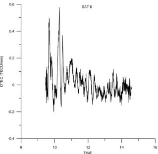
Figure 1. Vertical TEC variability (rate of change in TECU/min) due to a TID observed at Brussels along the track of satellite 6 on DOY 359 in 2004 (December 24 2004).
From this study, it appears that TEC smaller-scale variability at mid-latitude (in Europe) is mainly related to two types of phenomena : Travelling Ionospheric Disturbances (TID’s) or “noise-like” variability. TID’s appear as waves in the electron density which are due to interactions between the ionosphere and the neutral atmosphere. They have wavelengths ranging from a few km to more than thousand km and periods of a few minutes up to 3 hours. Figure 1 shows the variability in vertical TEC (vertical TEC rate of change) due to a TID detected at Brussels on DOY 359 in 2004 (December 24 2004). Let’s mention that the method proposed by Warnant et al. (2000) is only sensitive to TID’s with wavelengths smaller than about 100 km.
Figure 2. Noise-like variability in vertical TEC rate of change (in TECU/min) observed at Brussels during a severe geomagnetic storm on October 30 2003 along the track of satellite 1.
8 10 12 14 16 TIME -0.4 -0.2 0 0.2 0.4 0.6 D T EC ( T EC U /mi n ) SAT 6 1 2 3 4 5 6 7 TIME -0.8 -0.4 0 0.4 0.8 D T EC ( T EC U /m in ) SAT 1
Page 4 of 9
In mid-latitude stations, “noise-like” variability in TEC can also be observed. Such a variability is mainly detected during geomagnetic storms. Figure 2 shows “noise-like” variability in vertical TEC due to a severe geomagnetic storm observed at Brussels on DOY 303 in 2003 (October 30 2003). The signature of these “noise-like” structures in TEC is very similar to the signature of scintillations which are variations in phase and amplitude of GNSS signals due to the presence of irregularities in the ionosphere electron concentration. Scintillations are only observed in the equatorial and in the polar regions but noise-like variability observed at mid-latitude during severe geomagnetic storms can also induce strong degradations in GNSS differential applications.
Warnant et al. (2006-1), Warnant et al. (2006-2) and Hernandez-Pajares et al. (2006) analyse in details the ionospheric and geomagnetic conditions under which such a variability appears mainly based on ionograms, GPS-TEC and geomagnetic measurements.
3. SMALL-SCALE DISTURBANCE “CLIMATOLOGY”
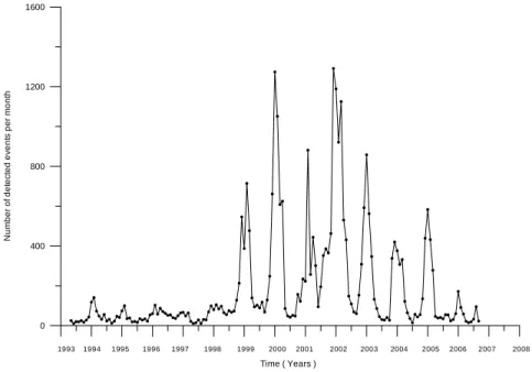
Figure 3 shows the number of “ionospheric events” (as defined above) detected at Brussels from April 1993 to August 2006. Most of these “events” are due to Travelling Ionospheric Disturbances (as already said, “noise-like” phenomena are mainly observed during geomagnetic storms).
Figure 3. Number of detected ionospheric events per month at Brussels from April 1993 to August 2006.
The analysis of Figure 3 shows that :
- TID’s are frequently observed all the time (during all seasons and during all phases of the 11-year Solar activity cycle).
- the number of detected events has an annual peak during winter time independently of Solar activity but the peak is much sharper at Solar maximum.
- the number of TID’s strongly depends on the Solar activity cycle: for example, about 200 events were observed in 1996, at Solar minimum when more than 1200 events were detected in January
Time ( Years ) 0 400 800 1200 1600 Num b e r of det ec ted e v ent s pe r m ont h 1993 1994 1995 1996 1997 1998 1999 2000 2001 2002 2003 2004 2005 2006 2007 2008
Page 5 of 9
2000 and January 2002 at Solar maximum (the 2 peaks which are present in Figure 3 correspond to the peaks of 2000 and 2002 observed in Solar Cycle 23).
TID’s have also a dependence on local time. In local winter, they are mainly observed during daytime around local noon. In the local summer, they are mainly observed during night time (figure 4).
Figure 4. Total number of ionospheric events detected per hour in January 2004 and in July 2006 in function of local time.
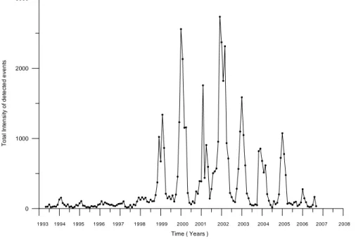
Figure 5 shows the total intensity (the sum of the intensities of all detected ionospheric events as defined in paragraph 2) of the ionospheric events per month detected at Brussels from April 1993 to August 2006.
Figure 5. Total intensity of detected ionospheric events per month at Brussels from April 1993 to August 2006. 0 4 8 12 16 20 24 Hour 0 10 20 30 40 50 Nu m b e r of ev ent s /hou r 0 4 8 12 16 20 24 Hour 0 5 10 15 20 25 Num ber of ev en ts /h o u r January 2004 July 2006 Time ( Years ) 0 1000 2000 3000 T o ta l I n tens it y of d e te c ted ev ent s 1993 1994 1995 1996 1997 1998 1999 2000 2001 2002 2003 2004 2005 2006 2007 2008
Page 6 of 9
A detailed analysis of the amplitudes of these ionospheric structures is under way. First results show that the largest (noise-like) gradients in TEC detected at Brussels during the period 2001-2006 were observed during severe geomagnetic storms on March 31 2001, October 30 2003 and November 20 2003 : in all 3 cases, vertical TEC variability up to 2.5 TECU/min was measured. The variability could even have been stronger during these events; indeed, above the threshold of 2.5 TECU/min, our software for the automatic detection of ionospheric variability failed to solve cycle slips in GNSS phase measurements and is therefore unable to monitor TEC variability. Further work (manual data editing) is necessary to fix this problem.
During the period 2001-2006, strong Travelling Ionospheric Disturbances were the origin of TEC variability up to 1.5 TECU/min. The strongest effects were detected in 2001 and 2002 at Solar maximum. Nevertheless, strong TID’s have also been detected during periods of “quiet” ionospheric conditions : a variability ranging from 0.6 to 1 TECU/min is very regularly observed even on days with very low values of TEC : for example, on December 24 2004, a variability of up to 0.6 TECU/min was observed when the mean and maximum daily TEC values were respectively of 5 TECU and 10 TECU what can be considered as representative of quiet background ionospheric conditions.
4. GRADIENTS IN SPACE DUE TO IONOSPHERIC SMALL-SCALE DISTURBANCES
As explained above, the single station method proposed by Warnant et al. (2000) detects small-scale ionospheric disturbances by monitoring TEC changes with time. Nevertheless, the influence of small-scale disturbances on GNSS differential applications depends on TEC gradients in space between the reference station and the user : this information is not directly supplied by the above-mentioned method. In practice, to assess the influence of small-scale ionospheric disturbances on differential positioning, we proceed in 2 steps: first, we detect periods with increased ionospheric variability with the single station method. Then, we analyse the gradients in space due to these ionospheric disturbances using the Belgian Active Geodetic Network : Belgium is equipped with network of 61 GNSS stations of which the role is to serve as reference for GNSS real time positioning applications on the Belgian territory. This network is one of the densest permanent networks in Europe : baseline lengths range between 4 km and about 20 km. This high density of stations allows to perform a detailed analysis of local TEC gradients in space over Belgium. For example, by forming double differences of phase observations collected in these stations of which the positions are precisely known, it is possible to monitor residual differential errors due to small-scale ionospheric disturbances.
Figure 6 and 7 illustrate the first results we have obtained with this methodology. Figure 6 shows double differences of L1 made with the data collected in the stations Brussels and Saint-Gilles (4 km) on December 24 2004 for 2 satellite pairs. These double differences are corrected for geometric terms (station and satellite positions). In other words, these double differences only contain the ambiguity term (which is an integer number) and non-modelled residual errors which are usually very small on a 4 km baseline (Warnant et al., 2006-3); this is the case in figure 6 (left) for satellite pair 28-27 where the double differences remain very close to the integer value of the ambiguity what means that residual errors are negligible. Double differences on satellite pair 21-6 show a very different behaviour (figure 6, right) : a TID, which has been detected on both satellite 21 and 6 using the single station method, is the origin of peak to peak variability of about 0.6 L1 cycles (11.5 cm) even on a short baseline of 4 km.
Page 7 of 9
Figure 6. Double difference of the L1 phase (in L1 cycles) on DOY 359 in 2004, baseline Brussels-Saint Gilles (4 km), satellite pair 28-27 (left) and satellite pair 21-6 (right).
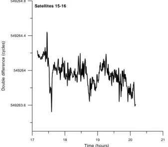
Figure 7. Double difference of the L1 phase (in L1 cycles) on DOY 324 in 2003, baseline Brussels-Saint Gilles, satellite pair 15-16.
As a second illustration, Figure 7 shows double differences (corrected for the geometric terms) on the baseline Brussels-Saint Gilles on November 20 2003 for satellite pair 15-16 for which noise-like variability has been detected (during a severe geomagnetic storm). Again, these small-scale structures in the ionosphere are the origin of peak to peak variability of about one L1 cycle (about 19 cm) on the 4 km baseline. On longer baselines, stronger differential ionospheric effects can be expected. Figure 8 shows the results obtained on DOY 359 in 2004 on the baseline Bertem-Mechelen (18 km) for the same
17 18 19 20 21 Time (hours) 549263.6 549264 549264.4 549264.8 D o ubl e di ff e renc e (c y c le s ) Satellites 15-16 11 12 13 14 15 16 Time (hours) 719726.8 719727.2 719727.6 719728 Do u b le d if fe re n c e ( cyc le s) Satellites 21-6 3.2 3.6 4 4.4 4.8 Time (hours) 1409606.8 1409607.2 1409607.6 1409608 D oubl e di ff e renc e ( c y c le s ) Satellites 28-27
Page 8 of 9
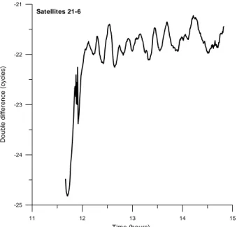
satellite pair (21-6) as in figure 6 for the 4 km baseline. As can be seen in this figure, peak to peak variability of more than 3 L1 cycles (60 cm) is observed in about 30 minutes due to the TID.
Figure 8. Double difference of the L1 phase (in L1 cycles) on DOY 359 in 2004, baseline Bertem-Mechelen (18 km), for satellite pair 21-6 .
These results should not be considered as worst-cases but just as first results obtained using the methodology outlined in this paper.
As a last remark, let’s recall that differential GNSS positions are obtained from the measurements made on all the satellites in view after a least-square adjustment procedure. Therefore, the effect of a TID or of noise-like variability on the final GNSS user position will depend on the number of satellites “affected” by the ionospheric disturbance and on the way the individual ionospheric errors for each observed satellite are “combined” in the least-square procedure. Therefore, figures 6, 7 and 8 do not give a direct assessment of the positioning error but give just an indication of it. Further work is necessary to obtain such a direct assessment.
5. CONCLUSIONS
GNSS differential applications are affected by small-scale structures in the ionosphere which are the origin of local gradients in TEC even on short distances of a few km.
In mid-latitudes stations in Europe, such gradients in TEC are due to Travelling Ionospheric Disturbances or to noise-like variability in TEC which follows geomagnetic storms. TID’s are detected all the time but their frequency of occurrence depends on Solar activity, on the season and on local time. They give rise to vertical TEC rate of change up to 1.5 TECU/min. The strongest TID’s occur at Solar maximum but strong TID’s can also be observed during quiet background ionospheric conditions. On the other hand, noise-like variability in vertical TEC reached the level of 2.5 TECU/min during severe geomagnetic storms on March 31 2001, October 30 2003 and November 20 2003. A more detailed study of these phenomena is ongoing. Let’s mention that these results can only be considered as representative of ionospheric conditions in mid-latitude European stations but that they could not be valid in other regions of the world.
11 12 13 14 15 Time (hours) -25 -24 -23 -22 -21 Do u b le d if fe renc e (c y c le s ) Satellites 21-6
Page 9 of 9
The gradients in space due to such ionospheric disturbances are studied based on the Belgian Active Geodetic Network where the distances between the reference stations range from 4km to about 20km. First results show that even on a 4 km baseline, TID’s can induce residual ionospheric errors of up to 0.6 cycles (11.5 cm) on double difference of L1 observations and noise-like variability can induce an error of up to 1 cycle (19 cm) during a severe geomagnetic storm. Larger effects are observed on longer baselines. Let’s highlight the fact that these values are first results which cannot be considered as worst-cases. On the other hand, specific impact on existing aviation standards cannot be evaluated until
further results are available.
6. RECOMMENDATION
The results may be considered while developing the mitigation technique for ionospheric effects on GNSS signals.
7. REFERENCES
Hernandez-Pajares M., Juan J. M., Sanz J., 2006, Medium-scale Travelling Ionospheric Disturbances affecting GPS measurements : spatial and temporal analysis, J. of Geoph. Res., Vol. 111, A07S11, doi:1029/2005JA011474.
Warnant, R., Pottiaux, E., 2000. The increase of the ionospheric activity as measured by GPS. Earth, Planets and Space, vol. 52(11), pp. 1055-1060.
Warnant, R., Kutiev, I., Marinov, P., Bavier, M., Lejeune, S., in press, 2006-1. Ionospheric and geomagnetic conditions during periods of degraded GPS position accuracy : 1. Monitoring variability in TEC which degrades the accuracy of Real Time Kinematic GPS application, Adv. Space Res.
Warnant, R., Kutiev, I., Marinov, P., Bavier, M., Lejeune, S., in press, 2006-2. Ionospheric and geomagnetic conditions during periods of degraded GPS position accuracy : 2. RTK events during disturbed and quiet geomagnetic conditions, Adv. Space Res.
Warnant, R., Lejeune, S., Bavier, M., in press, 2006-3. Space Weather influence on satellite-based navigation and precise positioning, Space Weather – Research towards Applications in Europe, Astrophysics and Space Science Library series, vol. 344, Ed. J. Lilensten, Springer.