1 2 3 4 5
A BAYESIAN APPROACH FOR MODELING 6
ORIGIN-DESTINATION MATRICES 7
8 9
Konstantinos Perrakis, Dimitris Karlis, Mario Cools, Davy Janssens and Geert Wets*
10 11
Transportation Research Institute 12 Hasselt University 13 Wetenschapspark 5, bus 6 14 BE-3590 Diepenbeek 15 Belgium 16 Fax.:+32(0)11 26 91 99 17 Tel:+32(0)11 26 9140 18 Email: [email protected] 19 20 Department of Statistics 21
Athens University of Business and Economics 22 76 Patision Str, 10434, Athens 23 Greece 24 Tel:+30 210 8203920 25 Email: [email protected] 26 27
Transportation Research Institute 28 Hasselt University 29 Wetenschapspark 5, bus 6 30 BE-3590 Diepenbeek 31 Belgium 32 Fax.:+32(0)11 26 91 99 33 Tel:+32(0)11 26 91{31, 28, 58} 34
Email: {mario.cools, davy.janssens, geert.wets}@uhasselt.be 35 36 Number of words: 6470 37 Number of Tables: 1 38 Number of Figures: 3 39
Total number of words: 6470 + 4*250 = 7470 40
41
Revised paper submitted: November 12, 2010 42
43 44
* Corresponding author 45
ABSTRACT 1
2
The majority of Origin Destination (OD) matrix estimation methods focus on situations 3
where weak or partial information, derived from sample travel surveys, is available. 4
Information derived from travel census studies, in contrast, covers the entire population of a 5
specific study area of interest. In such cases where reliable historical data exist, statistical 6
methodology may serve as a flexible alternative to traditional travel demand models by 7
incorporating estimation of trip-generation, trip-attraction and trip-distribution in one model. 8
In this research, a statistical Bayesian approach on OD matrix estimation is presented, where 9
modeling of OD flows, derived from census data, is related only to a set of general 10
explanatory variables. The assumptions of a Poisson model and of a Negative-Binomial 11
model are investigated on a realistic application area concerning the region of Flanders on the 12
level of municipalities. Problems related to the absence of closed-form expressions are 13
bypassed with the use of a Markov Chain Monte Carlo algorithm, known as the Metropolis-14
Hastings algorithm. Additionally, a strategy is proposed in order to obtain predictions from 15
the hierarchical, Poisson-Gamma structure of the Negative-Binomial model conditional on 16
the posterior expectations of the mixing parameters. In general, Bayesian methodology 17
reduces the overall uncertainty of the estimates by delivering posterior distributions for the 18
parameters of scientific interest as well as predictive distributions for future OD flows. 19
Predictive goodness-of-fit tests suggest a good fit to the data and overall results indicate that 20
the approach is applicable on large networks, with relatively low computational and 21
explanatory data-gathering costs. 22
1. INTRODUCTION 1
2
The OD matrix estimation problem is a well known problem in transportation analysis and a 3
crucial part of transportation planning. The existence of different schools of thought has 4
resulted to a diverse range of approaches dealing with the matter and therefore, OD 5
estimation methods vary significantly with respect to the modeling assumptions adopted and 6
the methodological tools utilized. Nevertheless, the selection of a specific OD estimation 7
method does not only depend on the methodological or philosophical framework or the 8
overall scope of research but also relies significantly on the amount and type of information 9
which is available. 10
Information for OD flows usually originates from travel surveys but is rarely used for 11
inferential purposes directly. As illustrated in Cools et al. (1), sample estimates of OD 12
matrices derived from travel surveys are biased even for large sampling rates and therefore 13
insufficient in delivering reliable estimates. Travel demand models, such as the four-step 14
model (2), take into account trip productions and trip attractions derived from travel surveys 15
and deliver more reliable OD estimates through gravity or entropy-maximization models 16
during the trip distribution step. Activity-based models, which form another trend in 17
transportation modeling (3), also use information from travel surveys in the model training 18
phase. Finally, methods which rely on observed link traffic counts, use OD matrices derived 19
from travel surveys as “prior” information in order to impose constraints and cope with the 20
under-specification problem between link flows and OD pairs (4). The last category of 21
methods constitutes the main body of existing research in OD matrix estimation and the 22
relative literature is extensive. A recent classification and discussion is provided by Timms 23
(5). Notable contributions within the Bayesian framework include the studies of Maher (6), 24
Tebaldi and West (7), Li (8), Castillo et al. (9) and Hazelton (10). 25
In contrast to research focused in OD matrix estimation from link traffic counts 26
and/or sample OD estimates, little or no research has been conducted for cases in which 27
historical OD data from census studies exist. OD matrices derived from census studies refer 28
to the population of a specific study area and therefore statistical methodology may be safely 29
utilized without necessarily linking the estimation problem to traffic counts. In addition, in 30
such cases statistical methodology may serve as an effective alternative to the widely used 31
travel demand models by integrating the steps of trip generation, trip attraction and trip 32
distribution into statistical models which deliver reliable parameter estimates and accurate 33
predictions. 34
In this current study, a statistical approach is presented where modeling is focused 35
directly on OD pairs derived from census data. The approach challenges some of the 36
practical and also methodological issues involved in OD matrix estimation, issues mainly 37
related to costs, extent of applicability and evaluation of uncertainty. Regarding cost-38
efficiency, the approach is in general not cost demanding since OD flows are explained only 39
by means of general and easily obtainable explanatory variables. The extent of applicability 40
is tested on a realistic study area, concerning the municipality network of the Northern, 41
Dutch-speaking part of Belgium, namely the region of Flanders which consists of 308 zones. 42
Finally, the main aim of the approach is to reduce the overall uncertainty of estimation. To 43
this extend, two models are investigated, a Poisson model and a Negative Binomial model. In 44
addition, the estimation is purely Bayesian and the Metropolis-Hastings algorithm, a Markov 45
Chain Monte Carlo algorithm, is used in order to acquire samples from the joint posterior 46
distribution of all parameters. Moreover, a strategy is suggested in order to obtain accurate 1
predictions of OD flows from the corresponding hierarchical Poisson-Gamma structure of 2
the Negative Binomial model. 3
As illustrated in the study, the proposed approach is applicable for networks of large 4
dimensionality, while at the same time data-gathering and computational costs are low. In 5
addition, Bayesian methodology reduces uncertainty over the randomness of OD flows in 6
two key aspects; first information is provided for the entire posterior distributions of the 7
parameters that influence OD flows and second prediction of future OD flows is similarly 8
based on predictive distributions instead of predictive point estimates. The former is useful in 9
obtaining a wider perspective over the factors that may help explain the generation and 10
attraction of OD trips. The latter, in combination with the inherent hierarchical nature of OD 11
matrices, facilitates transportation policy-making by providing predictive scenarios for traffic 12
volumes over multiple levels of aggregation and for different types of trips. Evaluation of 13
such scenarios by policy-makers reduces the uncertainty involved in decisions related to 14 transport infrastructure. 15 16 2. DATA 17 18 2.1 OD Matrix 19 20
The OD matrix is derived from the 2001 Belgian census, which contains information 21
about the departure/arrival times and locations of work and school trips for the 10,296,350 22
Belgian residents. The work and school trips are one-directional, from zone of origin to zone 23
of destination. Thus, the OD matrix contains the number of daily going-to-work/school 24
related trips for a normal weekday and for all travel modes. The area of concern in this study 25
is not the entire country of Belgium but the region of Flanders with a population of 6,058,368 26
residents. Information is provided on a highly analytic level, that is, the municipality network 27
of Flanders which consists of 308 zones. The resulting OD matrix contains 94,864 cells. 28
An important feature of OD matrices is their inherent hierarchical structure. An OD 29
matrix may be aggregated on different levels according to different geographical and/or 30
municipal classifications. For the region of Flanders, there are several levels of aggregation 31
that may be of interest; from the analytic level of municipalities to the more general levels of 32
cantons, districts, arrondissements and finally provinces. The hierarchical structure of 33
Flanders is represented below; on the higher level of municipalities the OD matrix has 308 34
zones and 94864 OD pairs whereas on the lower level of provinces there are only 5 zones 35
and 25 possible OD pairs, in between we find the levels of cantons, districts and 36
arrondissements. The downward direction of the arrows implies that each lower level is the 37
result of an aggregation on the immediately higher level. Therefore, having an OD estimate 38
on a high level of analysis is immediately advantageous, since it leads to direct OD estimates 39
for all the lower levels, whereas the opposite is not true. 40
Another characteristic of OD matrices is that the flows are usually inflated across the 41
main diagonal. The cells in the main diagonal correspond to “internal” trips; these are the 42
trips that are made within the same zone where there is no distinction between origin and 43 destination. 44 45 46
Municipalities 308×308 (94,864 cells) 1 ↓ 2 Cantons 103×103 (10,609 cells) 3 ↓ 4 Districts 52×52 (2,704 cells) 5 ↓ 6 Arrondissements 22×22 (484 cells) 7 ↓ 8 Provinces 5×5 (25 cells) 9 10
As expected, given the size of the matrix on municipality-level, the OD flows are 11
sparsely distributed. Approximately, 63% of the cells in the matrix are zero-valued. In 12
addition the data are clearly over-dispersed, since the mean of the OD flows equals 36.23 13
while the standard deviation is much larger, equal to 949.47. Finally, the cells across the 14
main diagonal correspond to approximately 43% of the total OD flows of the matrix and the 15
maximum value which is equal to 222,149 is observed in the diagonal cell belonging to 16
Antwerp, the capital and largest municipality of Flanders. 17
18
2.2 Explanatory Variables 19
20
The selection of the explanatory variables is a combination of variables that can be derived 21
immediately from the hierarchical structure of the OD matrix and of continuous explanatory 22
variables. The second category consists of variables such as employment ratios, population 23
densities, relative length of road networks, perimeter lengths of municipalities and yearly 24
traffic in highways and provincial/municipal roads. The set of explanatory variables is listed 25
below. 26
27
[1] dum.prov: dummy variable for internal-province trips
28
[2] dum.arron: dummy variable for internal-arrondissement trips
29
[3] dum.dist: dummy variable for internal-district trips
30
[4] dum.cant: dummy variable for internal-canton trips
31
[5] dum.munic: dummy variable for internal-municipality trips
32
[6] munic.cant: number of municipalities between the cantons of origin and destination
33
[7] munic.dist: number of municipalities between the districts of origin and destination
34
[8] munic.arron: number of municipalities between the arrondissements of origin and destination
35
[9] munic.prov: number of municipalities between the provinces of origin and destination
36
[10] empl.o: employment ratio of origin-zone
37
[11] empl.d: employment ratio of destination-zone
38
[12] pop.dens.o: population density of origin-zone (thousand inhabitants per square km)
39
[13] pop.dens.d: population density of destination-zone (thousand inhabitants per square km)
40
[14] road.length.o: length of road network relative to surface of origin-zone (km per square km)
41
[15] road.length.d: length of road network relative to surface of destination-zone (km per square km)
42
[16] perim.o: perimeter of origin-zone (in km’s)
43
[17] perim.d: perimeter of destination-zone (in km’s)
44
[18] HWT.o: km’s driven per year in highway roads of origin-zone (in millions)
45
[19] HWT.d: km’s driven per year in highway roads of destination-zone (in millions)
46
[20] PMT.o: km’s driven per year in provincial and municipal roads of origin-zone (in millions)
47
[21] PMT.d: km’s driven per year in provincial and municipal roads of destination-zone (in millions)
The variables which are extracted directly from the hierarchical structure of the OD matrix 1
are [1]-[9]. In particular, variables [1]-[5] are dummy variables indicating whether a trip is 2
internal or not for each level of aggregation, respectively. These variables are multiplied by 3
100 so that they correspond to a difference of one hundred trips. Variables [6]-[9] correspond 4
to the total number of municipalities belonging to the specific cantons, districts, 5
arrondissements and provinces of each OD pair. The rest [10]-[21], are the external 6
explanatory variables, which come in pairs, since they relate to origin as well as destination. 7
Finally, variables [6]-[21] are transformed in logarithmic scale, so that the multiplicative 8
interpretation of the models presented next remains on natural scale. 9
The set of the explanatory variables is in general simple, costless and also easy to 10
obtain. As mentioned, part of the explanatory variables is immediately derived by the 11
structure of the OD matrix. Variables related to populations, surfaces and perimeters are 12
usually available in transportation research centers and institutes. Finally, variables related to 13
length of road networks were obtained by the Belgian governmental website for statistics 14 (11). 15 16 3. MODELS 17 18
In this section, a brief description of the Poisson and Poisson-Gamma likelihood assumptions 19
is presented along with the selection of the corresponding prior distributions. Expressions for 20
the posterior distributions are then derived from the application of Bayes’ theorem. For 21
computational and notational convenience the OD flows are represented as a vector. Let n 22
denote the data size and p the number of explanatory variables. In addition, let 23
1 2
( ,y y ,...,yn)T
y denote the vector of OD flows, ( 0, 1, 2,..., ) T p β the vector of 24
unknown parameters and X the design matrix of dimensionality n(p1), containing the 25
intercept and the p explanatory variables, with ( 0, 1, 2,..., ) T i xi xi xi xip
x being the i-th row of
26
X related to OD flow y and i i1, 2,...n. 27
28
3.1 The Poisson Model 29
30
The likelihood assumption is that the OD flows are independently Poisson distributed, that is 31
| ~ ( )
i i
y β Pois for i1, 2,...n, where i is the Poisson mean for y , related to the i 32
explanatory variables through the log-link function log( ) T
i i
x β . The log-link function 33
implies the assumption that the effects of the explanatory variables are linear to the log-mean 34
of y . Consequently, the effects are exponential on natural scale, since i exp
Ti i
x β . The 35
complete likelihood is given by 36
37
1
exp exp exp
( | ) ! i y T T n i i i i p y
x β x β y β . (1) 38 39Poisson regression is a common option when modeling count data and it is frequently used in 40
practice. Nevertheless, Poisson models usually do not perform well in cases of over-41
dispersed data, since a strong restriction of Poisson modeling is that the mean is equal to the 42
variance of the data, that is E y
i|β
Var y
i|β
exp
x β . Properties and estimation Ti
1procedures for Poisson regression can be found in Agresti (12) and McCullagh and Nelder 2
(13), Bayesian applications are presented in Ntzoufras (14). 3
A flat non-informative prior with mean located at 0 and close-to-infinite variance is 4
assigned for parameter vector β . Specifically, the multivariate normal prior β~Np+1( ,0 Σβ), 5
with Σβ n
X XT
1103, which is one of the “benchmark” priors suggested in Fernández 6et al. (15). This prior distribution has the form 7 8
1 1 2 ( 1) 2 1 1 ( ) exp 2 2 T p p β β β β Σ β Σ . (2) 9 10By applying the Bayes’ theorem, the posterior distribution of β y is proportional to | 11
( | ) ( | ) ( )
p β y p y β p β . From expressions (1) and (2) the resulting posterior distribution is 12
13
11
1
( | ) exp exp exp exp .
2 i n y T T T i i i p
β β y x β x β β Σ β (3) 14 15Sampling directly from the posterior distribution is not feasible, since expression (3) does not 16
result in a known distributional form. 17
18
3.2 The Poisson-Gamma Model 19
20
The Poisson-Gamma model is a mixed Poisson regression model, where the mixing density 21
is assumed to be a Gamma distribution. Mixed Poisson models incorporate over-dispersion 22
and are frequently used as alternatives to the simple Poisson model (16). The likelihood 23
assumption is yi| ,β ui ~ Pois(iui), for i1, 2,...n , wherei is again the part of the Poisson 24
mean related to the explanatory variables through the log-link function log( ) T
i i x β and 25 1 2 ( , ,..., )T n u u u
u is a vector of random deviations or random intercepts distributed as 26
| ~ ( , )
i
u Gamma with , so that 0 E u . The Poisson likelihood is the
i 1 27conditional likelihood of y given the vector u; the complete conditional likelihood is given by 28
29
1
exp exp exp
( | , ) ! i y T T n i i i i i i u u p y
x β x β y β u . (4) 30 31From a Bayesian perspective the Poisson-Gamma model is an hierarchical model, since the 32
mixing distribution is regarded as a 1st level prior distribution for u and parameter is then 33
assigned a 2nd level prior distribution (14). 34
Alternatively, one may work with the marginal form of the model by integrating over 35
the mixing density; the integration p
y β| ,
p
y β u| ,
p u|
du results to a Negative-36Binomial marginal likelihood, that is yi| , ~β NB( , ) i , with iexp
x β for Ti
11, 2,...
i n. The complete marginal likelihood then, is 2 3
1 exp ( | , ) ! exp i i y T n i i y T i i i y p y
x β y β x β . (5) 4 5The mean of the data in this case is E y
i| ,β
exp
x βTi
, while the variance is 6
2 1| , exp T exp T
i i i
Var y β x β x β . Note that the variance now is a quadratic 7
function of the mean. Thus, Negative-Binomial regression incorporates over-dispersion, 8
since the assumed variance always exceeds the assumed mean. Information for the Negative-9
Binomial model can be found in Agresti (12) and McCullagh and Nelder (13). A general 10
Expectation-Maximization (EM) algorithm for obtaining Maximum Likelihood (ML) 11
estimates for mixed Poisson models, with emphasis on the Poisson-Gamma case, is provided 12
by Karlis (16). Within the Bayesian framework, Ntzoufras (14) presents descriptions and 13
applications for both the hierarchical and the marginal formulations of the model. 14
By means of Bayesian methodology, one might choose to fit either the hierarchical or 15
the marginal form of the model. In both cases, the estimates for the parameters of main 16
scientific interest, β and , will be the same due to the equivalence of the two models. The 17
hierarchical Poisson-Gamma model provides additional information over the posterior 18
distribution of u but it also requires estimation of the full set of parameters β u, and . The 19
marginal Negative-Binomial model on the other hand is simpler to fit, since estimation is 20
restricted to the reduced set of parameters and β . Due to the large size of the OD matrix, 21
fitting the hierarchical model in our case would prove to be a very difficult task which would 22
require estimating all of the 'su that correspond to the 94864 random intercepts. Instead, we i 23
choose to work with the simpler Negative-Binomial distribution. As we will see in section 24
5.2, information over the vector u is not completely lost and prediction from the hierarchical 25
structure is still feasible conditional on the posterior expectation of u. 26
Independent and non-informative priors are adopted for parameters β and . For 27
parameter vector β , the same multivariate normal distribution defined in expression (2) is 28
used. Regarding parameter , a Gamma a a distribution, with ( , ) 3 10
a
, as presented in 29
Ntzoufras (14) is chosen. The prior of is given by 30 31
1 ( ) exp ( ) a a a p a a . (6) 32 33Under the parameterization in expression (6) E( ) a a/ and 2
( ) /
Var a a . Thus, for 34
3 10
a the prior distribution of is a flat, non-informative distribution with mean equal to 35
1 and variance equal to 1000. 36
The joint posterior distribution of β, | y is now proportional to 37
( , | ) ( | , ) ( ) ( )
p β y p y β p β p , which leads to expression 38
1 1 1 exp 1 ( , | ) exp exp . 2 exp i i y T n i i T a y T i i y p a
β x β β y β Σ β x β (7) 1 2Inference from the posterior distribution is again not straightforward, since expression (7) 3
does not have a closed form solution. In the following section, we describe a Markov Chain 4
Monte Carlo method known as the Metropolis-Hastings algorithm, which is utilized in order 5
to generate samples from the posterior distributions in expressions (3) and (7). 6
7
4. METROPOLIS-HASTINGS IMPLEMENTATION 8
9
Markov Chain Monte Carlo (MCMC) methods are frequently used within the Bayesian 10
framework and are mainly employed in situations where the posterior distribution is not of 11
known form. The basic idea of MCMC is to initiate a Markov process from a specific starting 12
point and then iterate the process over a sufficient period of time. Due to the properties of 13
Markov processes, the resulting chain eventually converges to a stationary distribution which 14
is also the “target” posterior distribution. Once this is accomplished, an initial part of the 15
chain is discarded as part of the so-called “burn-in” period of the chain, which is the period 16
that the Markov chain has not yet reached convergence. The final result of MCMC is a 17
dependent sample from the posterior distribution, from which one may acquire summaries 18
for any posterior quantity of interest. Analytic information over the theoretical background 19
and applications of various MCMC algorithms can be found in Gamerman and Lopes (17) 20
and Gilks et al. (18). 21
Among the different types of MCMC methods, the Metropolis-Hastings (M-H) 22
algorithm is the most general method. The M-H algorithm is an iterative method, which 23
requires initially, specification of proposal distributions and of starting values for all 24
parameters included in a given model. The iterative procedure follows; at each iteration 25
draws of parameters are generated first from the proposal distributions, the draws are then 26
accepted or rejected according to a certain transition or acceptance probability. An extensive 27
description of the M-H algorithm is provided by Chib and Greenberg (19). 28
In particular, an independence-chain M-H algorithm is utilized where the location and 29
scale parameters of the proposal distribution remain fixed. The large data size results to 30
considerable time-consuming calculations and independence-chain M-H simulation proves to 31
perform faster than random-walk-chain M-H or other types of Metropolis-within-Gibbs 32
algorithms. The choice for the proposal distribution of parameter β , common in both the 33
Poisson and the Negative-Binomial model, is a multivariate normal distribution, 34
( ) ~ ( , )
q β Np+1 β Vβ , where β is the ML estimate of β and V is the estimated covariance β
35
matrix of β . For parameter of the Negative-Binomial model, the proposal distribution is 36
defined as q( ) Gamma a b( , ) , where parameters a and b are set to satisfy a b/ and 37
2
/
a b Var with being the ML estimate of . Having specified the proposal 38
distributions, the M-H algorithm for each model proceeds as presented below. 39
40 41 42
To simulate a M-H sample of size N for the Poisson model: 1
2
1) Set initial value β0 3
2) For iterations t1, 2,...,N: 4
a. Generate *
β from the proposal ( )q β 5
b. Calculate the transition probability
* 1 1 * ( | ) ( ) min ,1 ( | ) ( ) t MH t p q a p q β y β β y β 6
c. Generate a uniform random number u from U(0,1) 7 d. Set * 1 , if , if MH t t MH u a u a β β β 8 9
To simulate a M-H sample of size N for the Negative-Binomial model: 10
11
1) Set initial values 0
β and 0 12
2) For iterations t1, 2,...,N: 13
a. Generate *
β from the proposal q β and ( ) *
from the proposal ( )q 14
b. Calculate the transition probability
* * 1 1 1 1 * * ( , | ) ( ) ( ) min ,1 ( , | ) ( ) ( ) t t MH t t p q q a p q q β y β β y β 15
c. Generate a uniform random number u from U(0,1) 16 d. Set * * 1 1 ( , ) , if ( , ) ( , ) , if MH t t t t MH u a u a β β β 17 18
After certain preliminary tests, 5000 iterations for the Poisson model and 21000 19
iterations for the Negative-Binomial model were used in the final M-H runs, with resulting 20
acceptance ratios of 95% and 57%, respectively. The first 1000 iterations were discarded as 21
the “burn-in” part for both models. Convergence checks were based on the methods of 22
Raftery and Lewis (20), Geweke (21) and Heidelberger and Welch (22). The sample of the 23
Poisson model passed all the diagnostics, but due to memory limitations in calculations every 24
4th iteration was kept, resulting to a final sample of size 1000. Regarding the Negative-25
Binomial model, the diagnostic of Raftery and Lewis (20) indicated autocorrelation 26
problems. In order to break the strong autocorrelations, every 40th draw of the sample was 27
kept. For the final sample of 500 draws, all lag 1 autocorrelations were below 0.05. 28
29
5. RESULTS 30
31
In this section, results from the Poisson and Negative-Binomial regressions are summarized. 32
Posterior summaries, model comparison and plots of the posterior distributions are presented 33
first. A strategy for the Negative-Binomial model is suggested next, which allows to obtain 34
predictions from the corresponding Poisson predictive distribution. Several goodness-of-fit 35
tests are applied on the predictions and finally examples of predictive inference are 36
presented. 37
5.1 Posterior Inference 1
2
The results presented in this section, apply to the exponential parameters,Bj exp(j) for 3
0,1, 2,...21
j . The effect of these parameters on the mean OD flows is multiplicative on 4
natural scale and therefore interpretation is straightforward. For instance, posterior means 5
greater than 1 correspond to an increasing multiplicative effect, whereas posterior means less 6
than 1 have a decreasing multiplicative effect. 7
Posterior means, standard deviations and 95% probability intervals for parameters B j 8
and parameter are summarized in Table 1. 9
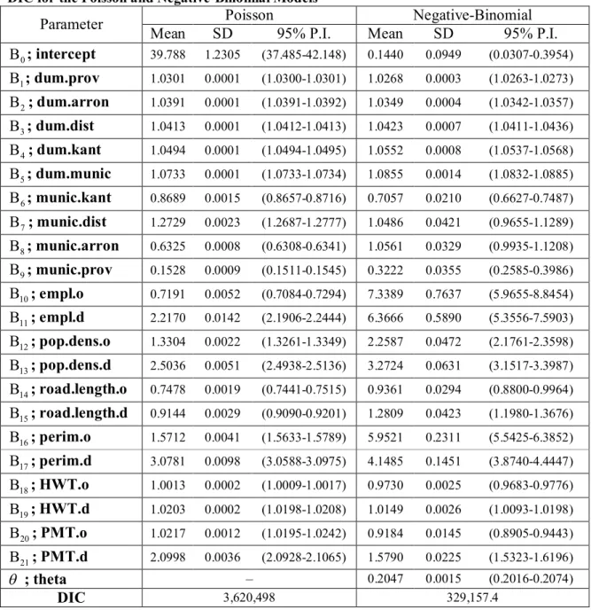
10
TABLE 1 Posterior Means, Standard Deviations, 95% Probability Intervals and the Values of
11
DIC for the Poisson and Negative-Binomial Models
12
Poisson Negative-Binomial
Parameter
Mean SD 95% P.I. Mean SD 95% P.I.
0 ; intercept 39.788 1.2305 (37.485-42.148) 0.1440 0.0949 (0.0307-0.3954) 1 ; dum.prov 1.0301 0.0001 (1.0300-1.0301) 1.0268 0.0003 (1.0263-1.0273) 2 ; dum.arron 1.0391 0.0001 (1.0391-1.0392) 1.0349 0.0004 (1.0342-1.0357) 3 ; dum.dist 1.0413 0.0001 (1.0412-1.0413) 1.0423 0.0007 (1.0411-1.0436) 4 ; dum.kant 1.0494 0.0001 (1.0494-1.0495) 1.0552 0.0008 (1.0537-1.0568) 5 ; dum.munic 1.0733 0.0001 (1.0733-1.0734) 1.0855 0.0014 (1.0832-1.0885) 6 ; munic.kant 0.8689 0.0015 (0.8657-0.8716) 0.7057 0.0210 (0.6627-0.7487) 7 ; munic.dist 1.2729 0.0023 (1.2687-1.2777) 1.0486 0.0421 (0.9655-1.1289) 8 ; munic.arron 0.6325 0.0008 (0.6308-0.6341) 1.0561 0.0329 (0.9935-1.1208) 9 ; munic.prov 0.1528 0.0009 (0.1511-0.1545) 0.3222 0.0355 (0.2585-0.3986) 10 ; empl.o 0.7191 0.0052 (0.7084-0.7294) 7.3389 0.7637 (5.9655-8.8454) 11 ; empl.d 2.2170 0.0142 (2.1906-2.2444) 6.3666 0.5890 (5.3556-7.5903) 12 ; pop.dens.o 1.3304 0.0022 (1.3261-1.3349) 2.2587 0.0472 (2.1761-2.3598) 13 ; pop.dens.d 2.5036 0.0051 (2.4938-2.5136) 3.2724 0.0631 (3.1517-3.3987) 14 ; road.length.o 0.7478 0.0019 (0.7441-0.7515) 0.9361 0.0294 (0.8800-0.9964) 15 ; road.length.d 0.9144 0.0029 (0.9090-0.9201) 1.2809 0.0423 (1.1980-1.3676) 16 ; perim.o 1.5712 0.0041 (1.5633-1.5789) 5.9521 0.2311 (5.5425-6.3852) 17 ; perim.d 3.0781 0.0098 (3.0588-3.0975) 4.1485 0.1451 (3.8740-4.4447) 18 ; HWT.o 1.0013 0.0002 (1.0009-1.0017) 0.9730 0.0025 (0.9683-0.9776) 19 ; HWT.d 1.0203 0.0002 (1.0198-1.0208) 1.0149 0.0026 (1.0093-1.0198) 20 ; PMT.o 1.0217 0.0012 (1.0195-1.0242) 0.9184 0.0145 (0.8905-0.9443) 21 ; PMT.d 2.0998 0.0036 (2.0928-2.1065) 1.5790 0.0225 (1.5323-1.6196) ; theta – 0.2047 0.0015 (0.2016-0.2074) DIC 3,620,498 329,157.4
Statistical significance may be checked directly upon examination of the 95% 1
posterior probability intervals. Regarding parameters B of the Poisson model, none of the j 2
corresponding posterior intervals includes the value of 1, consequently all parameters have 3
significant effects. In the Negative-Binomial model parameters B and 7 B do not seem to 8 4
have a significant effect. The rest of the regression parameters are significant. For the case of 5
dispersion parameter of the Negative-Binomial model, the posterior interval does not 6
support the value of zero, therefore parameter is also significant. Based on the posterior 7
means of regression parameters B , the parameters that seem to have a greater impact, j 8
especially in the Negative-Binomial model, are B , 10 B , 11 B , 12 B , 13 B and 16 B , which 17 9
correspond to the effects of employment ratio, of population density and of perimeter length 10
for the zones of origin and destination, respectively. Finally, parameter B corresponding to 21 11
the effect of yearly traffic in provincial/municipal roads of destination zones is also strongly 12
influential in both models. 13
In addition to posterior point estimates and intervals presented in Table 1, direct 14
examination of the posterior distribution often provides extra information and a more 15
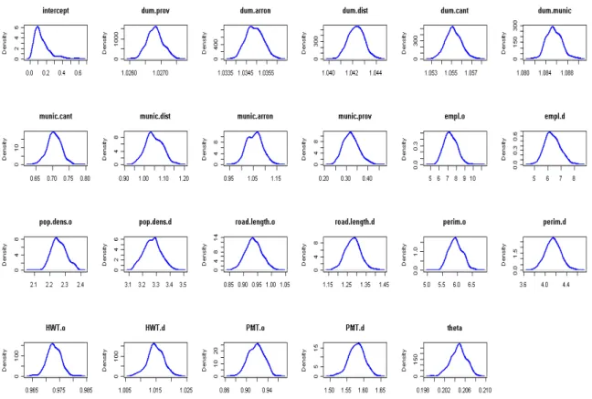
comprehensive view regarding the random nature of parameters. Kernel smoothed estimates 16
of the 23 posterior distributions for the parameters of the Negative-Binomial model are 17
presented in Figure 1. 18
19
FIGURE 1 Kernel posterior distribution estimates for the parameters of the Negative-Binomial
20
model.
21 22
Model comparison is based on the Deviance Information Criterion (DIC), introduced 1
by Spiegelhalter et al. (23). The DIC is a model selection criterion, useful in determining the 2
best model within a specific group of models. Based on the DIC support is given to the 3
model with the lowest resulting value. The DIC values for the two models are also shown in 4
Table 1, indicating that the value of the Negative-Binomial model is much lower than the 5
corresponding value of the Poisson model. Consequently, according to the DIC, the 6
Negative-Binomial model clearly outperforms the simple Poisson model. Evidently, the latter 7
does not provide a good fit to the data due to the strong presence of over-dispersion. This is 8
in accordance with the finding that parameter , which accounts for the extra variability, is 9 statistically significant. 10 11 5.2 Prediction 12 13
According to a lemma provided by Sapatinas (24), if y| , ~ u Pois(u) and u has a 14
probability function G , i.e. ( ) u~G u , then, posterior expectations of u can be derived ( ) 15
from the formula 16 17
|
( )! ( ) ! ( ) r G r G p y r y r E u y, y p y , (8) 18 19where p is the probability function of the corresponding mixed Poisson distribution. G( ) 20
Expression (8) holds for all cases of mixed Poisson models. The formula is also utilized by 21
Karlis (16) in a general EM algorithm for mixed Poisson models. 22
In our context, the mixed Poisson distribution corresponds to the Negative-Binomial 23
distribution, denoted previously as ( | , )p y β and given in expression (5). It is then possible, 24
given formula (8), to obtain a sample of posterior expectations of u; let (l) be an indicator for 25
the 500 MCMC draws, then, by setting in (8) r 1 and by “plugging-in” the MCMC draws 26
( )l
β , ( )l , for l 1, 2,...500, we obtain posterior expectations of u as follows 27 28
( ) ( ) ( ) ( ) ( ) ( ) ( ) ( 1)! ( 1 | , ) | , exp( ) ! ( | , ) l l l l l l l p E , p EXP y y β u u y β Xβ y y β . (9) 29 30Now, predictions of OD flows can be generated from the Poisson distribution conditional on 31
β and uEXP; for each ( )l
β and u( )EXPl , with l 1, 2,...500, we generate one predictive dataset
32 ( ) pred l y from 33 ( ) ( ) ( ) ~ ( ) pred l l l Pois EXP y β u . (10) 34 35
Each one of the 500 ypred 's, consists of one predictive OD matrix for Flanders. Predictions 36
from the Poisson distribution, unlike predictions from the Negative-Binomial distribution, 37
take into account the specific random intercept of each OD flow. The proximity of these 38
predictions with respect to the original dataset is investigated next. 39
40 41
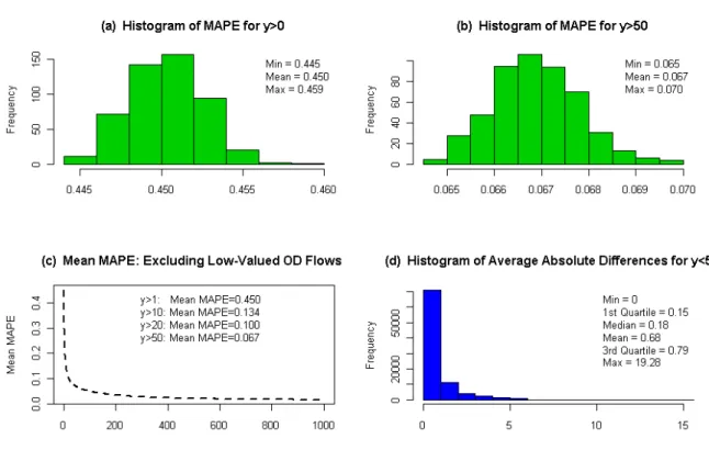
5.3 Goodness-of-fit 1
2
In order to evaluate the goodness-of-fit of the Negative-Binomial model, several measures of 3
fit are considered. A measure frequently used within the transportation field is initially 4
calculated. Bayesian methodology enhances the information provided by the measure, since 5
the outcome is once again a distribution estimate rather than a point estimate. Evaluation of 6
the fit is then supplemented by statistical tests based on Bayesian p-values. 7
The distance between the predictive datasets and the initial dataset is assessed by the 8
Mean Absolute Percentage Error (MAPE) measure, which corresponds to an average 9
percentage of deviation from the initial dataset. By definition, the calculation of MAPE 10
cannot include the zero-valued cells of the OD matrix. Nevertheless, in large OD matrices, 11
small or even medium deviations from zero-valued cells are usually not influential. If we 12
denote with m the total number of cells which are not zero and with k an indicator 13
1, 2,...
k m for y , then, we obtain 500 corresponding MAPE values from k 0 14 15 ( ) ( ) 1 pred l m l k k k k y y MAPE m y
, 16 17for l 1, 2,...,500. The resulting mean value of MAPE is 0.45, with a minimum of 0.445 and 18
a maximum of 0.459. The mean MAPE seems relatively high, corresponding to a 45% 19
deviation from the initial dataset. Nevertheless, this value is slightly misleading due to the 20
fact that MAPE is also highly influenced from small deviations in low-valued cells. 21
Excluding categories of low-valued cells in the calculation of MAPE, reveals that the mean 22
value decreases drastically; the value of the mean MAPE for OD flows greater than 10 is 23
decreased to 0.134 and for OD flows which are greater than 20 the corresponding value 24
becomes 0.1. Finally, for OD flows greater than 50 the mean is 0.067, with a minimum of 25
0.065 and a maximum of 0.07. These results are summarized in the plots of Figure 2; as we 26
observe in plot (c) the mean of MAPE is decreasing steadily and the deviations from the 27
initial dataset become almost negligible for medium and large valued cells. 28
According to MAPE the Negative-Binomial models performs well for prediction of 29
medium and large OD flows. The 6.7% deviation for OD flows greater than 50 is already 30
small. Yet, MAPE is not very informative concerning the fit of the model in low-valued cells, 31
since small deviations, which may not be significant in practical terms have a high influence 32
in the calculation of the measure. A direct way of evaluating the fit in low-valued cells is to 33
simply calculate the absolute differences between the initial and the predictive datasets. Plot 34
(d) in Figure 2 is a histogram with a summary of the average absolute differences for OD 35
flows equal to or less than 50. Note that the differences are not large; the mean equals 0.68, 36
50% are equal to or less than 0.18, 75% are equal to or less than 0.79 and the maximum 37
absolute difference is 19.28. 38
1
FIGURE 2 Histogram of MAPE (a), histogram of MAPE for OD flows greater than 50 (b), plot
2
of the mean values of MAPE resulting by excluding low-valued cells (c) and histogram of the
3
average absolute differences for OD flows equal or less than 50 (d).
4 . 5
In addition to the previous analysis, two extra measures of discrepancy between the 6
predictions of the model and the data are considered; the absolute distances and the squared 7
distances of the initial and the predictive data from the corresponding expected values of the 8
model. In Bayesian terms, the measures are identified as test quantities which are evaluated 9
by means of Bayesian p-values. A Bayesian p-value should ideally equal 0.5, extreme values 10
very close to 0 or 1 suggest failure of a model in the specific aspect that is investigated by the 11
test quantity (25). The Bayesian p-value was initially defined by Rubin (26), several 12
examples for the use of test quantities and interpretation of Bayesian p-values are presented 13
in Gelman et al. (25). Following the terminology used by Gelman et al. (25) we denote the 14
two test quantities as 15
1 1 2 2 1 Absolute-Distance: ( , , ) ( | , ) Squared-Distance: ( , , ) ( | , ) . n i i i n i i i T y E y T y E y
y β β θ y β β θ 16 17The resulting Bayesian p-value is 0 for the Absolute-Distance quantity, indicating a bad fit, 18
and 0.488 for the Squared-Distance quantity which actually suggests a very good fit. The 19
result at first glance seems contradictive, nevertheless it is in accordance with the previous 20
findings. The Absolute-Distance is a strict measure which assigns more penalty to small 21
deviations, while the Squared-Distance measure gives more weight to large deviations from 22
the data. Like MAPE, the Absolute-Distance measure is influenced by small deviations, 1
especially in low-valued cells. Given the size of the data, the cumulative effect of these 2
deviations appears to be statistically significant under certain strict measures, yet in practical 3
terms the overall effect is not significant. In our case, the Squared-Distance measure seems a 4
more suitable test quantity for evaluating goodness-of-fit. 5
6
5.4 Predictive Inference 7
8
The 500 datasets generated from the predictive distribution in expression (10) may now be 9
used in various types of predictions of traffic volumes. As mentioned in section 2.1, 10
modeling on the level of municipalities allows for prediction on other levels of aggregation 11
as well. For instance, predictions for OD flows between districts can be derived directly as 12
summations of the predictions for OD flows between municipalities. Thus, predictive 13
inference is not necessarily restricted on the level of municipalities; it can be applied on any 14
other hierarchical level, such as the levels of cantons, districts, arrondissements and 15
provinces. In addition, prediction may also be focused on specific types of traffic volumes 16
that might be of interest, e.g. strictly in-coming trips, strictly out-coming trips or just internal 17
trips. 18
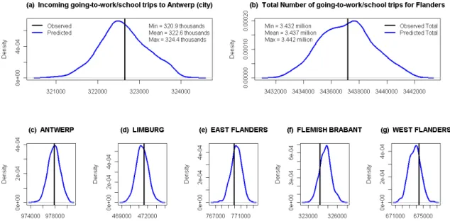
In Figure 3, applications of prediction on different levels of aggregation and for 19
different types of trips are demonstrated. The applications correspond to predictions for the 20
total number of in-coming, going-to-work/school trips from all other municipalities to the 21
capital of Flanders, Antwerp, predictions for the total number of going-to-work/school trips 22
that occur daily in the whole region of Flanders and finally predictions for the daily internal 23
going-to-work/school trips that take place in each one of the five Flemish provinces. 24
25
FIGURE 3 Going-to-work/school trip predictive distributions for incoming trips to Antwerp
26
(a), for total number of trips in Flanders (b) and for internal trips within each of the five
27
Flemish provinces; Antwerp (c), Limburg (d), East Flanders (e), Flemish Brabant (f) and West
28
Flanders (g). The vertical black lines indicate the corresponding observed quantities.
29 30
Similar predictive distributions can be derived for any case of specific OD flows that 1
might be of particular interest. It is worth noting, that these predictions also serve as further 2
goodness-of-fit tests, since in every case there is a corresponding observed quantity to 3
compare with. In the applications above, the observed quantities are represented with vertical 4
black lines. As illustrated in Figure 3, all observed quantities are well within high-density 5
regions of the corresponding predictive distributions, an indication that the predictions are 6
not extreme with respect to the initial data. 7
In general, the predictive distributions provide all the necessary information 8
concerning the variability of future traffic flows. The predictive effects may be examined 9
under different assumptions; one might choose to infer based on conservative summaries 10
such as the predictive mean or median, or one might be interested in examining the effect of 11
more extreme summaries such as the 99th percentile or the maximum value. These alternative 12
options reduce overall uncertainty and may serve as predictive scenarios for transportation 13
policy-makers, e.g. in decisions concerning infrastructure expansion. 14
15
6. CONCLUSIONS AND DISCUSSION 16
17
In this paper, OD matrix estimation from census data was investigated from a Bayesian 18
modeling perspective. Applications of a Poisson model and of a Negative-Binomial model 19
were presented for the municipality network of Flanders. All of the regression parameters of 20
the Poisson model and most of the parameters of the Negative-Binomial model including the 21
dispersion parameter proved to be statistically significant. Model comparison based on the 22
DIC indicated that Negative-Binomial regression is a more suitable choice than simple 23
Poisson regression due to the great degree of over-dispersion present in OD flows. Finally, 24
predictions were obtained from the corresponding hierarchical structure of the Negative-25
Binomial model, conditional on the posterior expectation of the mixing parameters. The 26
proximity of these predictions with respect to the initial data was evaluated according to 27
several measures of discrepancy. The overall fit was found to be satisfactory. 28
A novel application emerges as a direct extension of the proposed methodology. The 29
application entails using the predictive output of a certain model as input to a specific 30
assignment method. That would allow for predictions on the level of link flows and also 31
provide the opportunity to additionally compare observable link flows with respect to the 32
corresponding predictive distributions. 33
Future research may focus further on the selection of explanatory variables. The 34
choice of explanatory variables used, should be viewed as a first attempt and not as a 35
concluding proposition. Expanding the models, by including appropriate explanatory 36
variables that influence the generation and attraction of trips, is a matter of ongoing research. 37
For instance, variables related to distances and coordinates proved to be highly significant in 38
experiments of smaller scale and will be included in future results. 39
Uncertainty over model choice also provides space for further investigation. The class 40
of mixed Poisson distributions, results to several potential models that might be reasonable 41
candidates for OD matrix modeling. The widely used Poisson-Log Normal model, for 42
example, appearing more frequently in the relative literature as a Poisson model with 43
normally distributed random effects, is a possible alternative to the Poisson-Gamma model. 44
A less known alternative belonging to the same class, is the Poisson-Inverse Gaussian 45
regression model. 46
Finally, it is arguable that the proposed methodology may serve as an effective 1
alternative to the traditional four-step transportation model for cases in which historical OD 2
data exist. From this point of view the methodology may be seen as a joint trip generation, 3
trip attraction and trip distribution method which integrates the first two phases of a four-step 4
model in one statistical model with wider predictive capabilities. 5
REFERENCES 1
2
(1) Cools, M., E. Moons, and G. Wets. Assessing Quality of Origin-Destination Matrices 3
Derived from Activity and Travel Surveys: Results from a Monte Carlo Experiment. 4
Forthcoming in Transportation Research Record: Journal of the Transportation 5
Research Board, 2010. 6
(2) Hensher, D.A. and K.J. Button. Handbook of transport modelling. Elsevier Ltd., 7
London, 2000. 8
(3) Henson, K., K. Goulias, and R. Golledge. An assessment of activity-based modeling 9
and simulation for applications in operational studies, disaster preparedness, and 10
homeland security. Transportation Letters: The International Journal of Transportation 11
Research, vol. 1, 2009, pp. 19-39. 12
(4) Abrahamsson, T. Estimation of Origin-Destination Matrices Using Traffic Counts – A 13
Literature Survey. IIASA Interim Report IR-98-021, 1998. 14
(5) Timms, P. A philosophical context for methods to estimate origin destination trip 15
matrices using link counts. Transport Reviews: A Transnational Transdisciplinary 16
Journal, Vol. 21, No. 3, 2001, pp. 269-301. 17
(6) Maher, M.J. Inferences on trip matrices from observations on link volumes: A Bayesian 18
statistical approach. Transportation Research Part B: Methodological, Vol. 17, 1983, 19
pp. 435-447. 20
(7) Tebaldi, C. and M. West. Bayesian Inference on Network Traffic Using Link Count 21
Data. Journal of the American Statistical Association, Vol. 93, 1996, pp. 557-576. 22
(8) Li, B. Bayesian Inference for Origin-Destination Matrices of Transport Networks Using 23
the EM Algorithm. Technometrics, Vol. 47, 2005, pp. 399-408. 24
(9) Castillo, E., J.M. Menéndez, and S. Sánchez-Cambronero. Predicting traffic flow using 25
Bayesian networks. Transportation Research Part B: Methodological, Vol. 42, 2008, 26
pp. 482-509. 27
(10) Hazelton, M.L. Bayesian inference for network-based models with a linear inverse 28
structure. Transportation Research Part B: Methodological, Vol. 44, 2010, pp. 674-29
685. 30
(11) FOD Economie, FOD Economie - SPF Economie - Statbel. www.statbel.fgov.be. 31
Accessed February 22, 2010. 32
(12) Agresti, A. Categorical Data Analysis, Second edition. John Wiley and Sons, Inc., 33
Hoboken, New Jersey, 2002. 34
(13) McCullagh, P. and J.A. Nelder. Generalized Linear Models, Second Edition. Chapman 35
and Hall/CRC, London, 1989. 36
(14) Ntzoufras, I. Bayesian Modeling Using WinBUGS. John Wiley and Sons, Inc., 37
Hoboken, New Jersey, 2009. 38
(15) Fernández, C., E. Ley, and M.F.J. Steel. Benchmark priors for Bayesian model 39
averaging. Journal of Econometrics, Vol. 100, 2001, pp. 381-427. 40
(16) Karlis, D. A general EM approach for maximum likelihood estimation in mixed Poisson 41
regression models. Statistical Modelling, Vol. 1, No. 1, 2001, pp. 305-318. 42
(17) Gamerman, D. and H.F. Lopes. Markov Chain Monte Carlo: Stochastic Simulation for 43
Bayesian Inference, Second Edition. Chapman and Hall/CRC, London, 2006. 44
(18) Gilks, W., S. Richardson, and D. Spiegelhalter. Markov Chain Monte Carlo in Practice: 45
Interdisciplinary Statistics. Chapman and Hall/CRC, London, 1995. 46
(19) Chib, S. and E. Greenberg. Understanding the Metropolis-Hastings Algorithm. The 1
American Statistician, Vol. 49, No. 4, 1995, pp. 335-327 2
(20) Raftery, A.E. and S. Lewis. How Many Iterations in the Gibbs Sampler? In Bayesian 3
Statistics, Vol. 4, 1992, pp. 763-773. 4
(21) Geweke, J. Evaluating the Accuracy of Sampling-Based Approaches to the Calculation 5
of Posterior Moments. In Bayesian Statistics, Vol. 4, 1992, pp. 169-193. 6
(22) Heidelberger, P. and P.D. Welch. Simulation Run Length Control in the Presence of an 7
Initial Transient. Operations Research, Vol. 31, 1983, pp. 1109-1144. 8
(23) Spiegelhalter, D.J., N.G. Best, B.P. Carlin, and A.V.D. Linde. Bayesian measures of 9
model complexity and fit. Journal Of The Royal Statistical Society Series B, Vol. 64, 10
No. 4, 2002, pp. 583-639. 11
(24) Sapatinas, T. Identifiability of mixtures of power-series distributions and related 12
characterizations. Annals of the Institute of Statistical Mathematics, Vol. 47, No. 3, 13
1995, pp. 447-459. 14
(25) Gelman, A., J.B. Carlin, H.S. Stern, and D.B. Rubin. Bayesian Data Analysis, Second 15
Edition. Chapman & Hall, London, 2003. 16
(26) Rubin, D.B. Bayesianly Justifiable and Relevant Frequency Calculations for the 17
Applied Statistician. The Annals of Statistics, Vol. 12, No. 4, 1984, pp. 1151-1172. 18