Fuzzy interpolation and level 2 gradual rules

HAL Id: hal-00482900

https://hal.archives-ouvertes.fr/hal-00482900

Submitted on 11 May 2010

HAL is a multi-disciplinary open access archive for the deposit and dissemination of sci-entific research documents, whether they are pub-lished or not. The documents may come from teaching and research institutions in France or abroad, or from public or private research centers.

L’archive ouverte pluridisciplinaire HAL, est destinée au dépôt et à la diffusion de documents scientifiques de niveau recherche, publiés ou non, émanant des établissements d’enseignement et de recherche français ou étrangers, des laboratoires publics ou privés.

Fuzzy interpolation and level 2 gradual rules

Sylvie Galichet, Didier Dubois, Henri Prade

To cite this version:

Sylvie Galichet, Didier Dubois, Henri Prade. Fuzzy interpolation and level 2 gradual rules. EUSFLAT’03, Sep 2003, Zittau, Germany. pp. 506-511. �hal-00482900�

Abstract

Functional laws may be known only at a fi-nite number of points, and then the function can be completed by interpolation tech-niques obeying some smoothness condi-tions. We rather propose here to specify constraints by means of gradual rules for de-limiting areas where the function may lie be-tween known points. Such an approach results in an imprecise interpolation graph whose shape is controlled by tuning the fuzziness attached to the reference points. However, the graph so-built is still crisp, which means that different possible paths between the interpolation points cannot be distinguished according to their plausibility. The paper discusses a method for introduc-ing membership degrees inside the interpo-lation graph. The developed formalism relies on the use of weighted nested graphs. It amounts to handling level 2 gradual rules for specifying a family of flexible con-straints on the reference points. The pro-posed approach is compared with the one of extending gradual rules for dealing with type 2 fuzzy reference points.

Keywords: Gradual rules, Fuzzy interpola-tion, Level 2 fuzzy sets

1 Introduction

The main purpose of this paper is to further investi-gate the interest of gradual rules [5] for modelling in-terpolative reasoning. What is supposed to be known, in a precise or in an imprecise way, is the behaviour of a system at some points or in some areas, the problem being to interpolate between these regions. The pro-posed rule-based approach is an alternative to works based on fuzzy polynomial [10] or fuzzy spline inter-polation [9], [1], which rely on fuzzy-valued

func-tions. Using such techniques, fuzzy interpolation depends on the analytical form of the interpolant (lin-ear, polynomial, spline-based).

Using a rule-based formalism, we are no longer look-ing for a function, possibly fuzzy, but for a relation linking input variables to output variables, still con-strained by the points which govern the interpolation. Actually, each constraint is expressed by a rule that encapsulates the underlying reference point. This principle was developed in [7], then applied to impre-cise modeling for the classification of time series [8]. In these first attempts, the built interpolation graphs are imprecise but still crisp. Actually, the fuzziness in-troduced for modeling closeness with respect to pre-cise interpolation points is not present in the interpolation graph. This paper presents a refinement of the rule-based representation that enables the han-dling of fuzzy interpolation graphs. The proposed method consists in implementing level 2 gradual rules.

The paper, after some brief background on gradual rules, discusses interpolation between precisely known points. Then, the building of nested interpola-tive graphs is addressed. Their weighting allows the definition of fuzzy graphs as level 2 fuzzy sets of crisp graphs. Finally, it is shown that similar results can be obtained using a type 2 fuzzy set-based approach.

2 Interpolation and gradual rules

In the one-dimensional input case considered in the paper, the input-output relation is represented by its graph Γ defined on the Cartesian product X x Z (where X is the input domain, and Z the output domain). The idea of imprecise interpolation suggested above is based on constraints to be satisfied, namely the postu-late that the results of the interpolation should agree with the interpolation points. These constraints should be expressed in order to define the graph Γ of the relation on X x Z.

Fuzzy interpolation and level 2 gradual rules

Sylvie Galichet 1,2 Didier Dubois1 Henri Prade1

1 _{IRIT, Université Paul Sabatier, 118 route de Narbonne, 31062 Toulouse Cedex 4} 2 _{LISTIC, Université de Savoie, 41 avenue de la plaine, BP806, 74016 Annecy Cedex}

We consider the case of precise interpolation points P_i with coordinates (x_i, z_i), i = 1, ..., n. Then the relation

Γ should satisfy:

Γ(x_i, z_i) = 1,

∀ z≠z_i ∈Z, Γ(x_i, z) = 0,

for i = 1, ..., n. Without any further constraint on the nature of the interpolation, we only have:

∀ x≠x_i ∈X, ∀ z∈Z, Γ(x, z) = 1.

Thus each interpolation point induces the constraint “If x = x_i then z = z_i”, represented by (x = x_i) → (z = z_i) where → is the material implication. The relation

Γ is thus obtained as the conjunction:

Γ(x, z) = ∧ _{i = 1, .., n} (x = x_i) → (z = z_i). (1) This relation is extremely imprecise since there is no constraint at all outside the interpolation points. The absence of a choice of a precise type of interpolation function should be alleviated by the use of fuzzy rules in order to express constraints in the vicinity of the in-terpolation points. The idea is to use rules of the form “the closer x is to x_i, the closer z is to z_i” [5]. The ex-tension to gradual rules of equation (1) provides the following expression for the graph Γ:

Γ(x, z) = min_{i = 1, .., n}µ_{close to xi}(x) → µ_{close to zi}(z)(2) where → represents Rescher-Gaines implication, i.e. a → b = 1 if a ≤ b and a → b = 0 if a > b, and the value

µ_{close to xi}(x) is the degree of truth of the proposition “x is close to x_i”.

Two comments on equation (2) are worth stating. First, the principle underlying the rules is the one at work in analogical or case-based reasoning and (2) is interpreting this principle as a constraint (as opposed to a weaker interpretation leading to Mamdani-like fuzzy systems, see [3]). Moreover, (2) embeds inter-polation in a purely logical setting (see [2]) which does not require a defuzzification step.

We have now to define what is meant by “close to”. Let A_i denote the fuzzy set of values close to x_i. It is natural to set µ_Ai(x) = 1 if x = x_i and to assume that the membership degree to A_i decreases on each side of x_i with the distance to x_i. The simplest solution consists in choosing triangular fuzzy sets with a support denot-ed by [x_i−, x_i+]. In a similar way, the closeness to z_i will be modelled by a triangular fuzzy set B_i with mo-dal value z_i and support [z_i−, z_i+]. Then the interpola-tion relainterpola-tion only depends on 4n parameters x_i−, x_i+,

z_i−, z_i+ for n interpolation points.

We might think of using a strong fuzzy partition both for X and Z (i.e. ∀x∈X, Σ_{i=1, ..., n} µ_Ai(x) = 1 and ∀z∈Z,

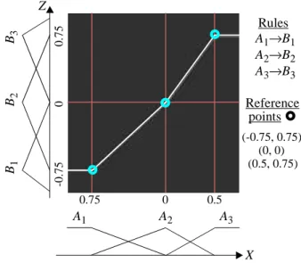
Σ_{i=1, ..., n} µ_Bi(z) = 1), with triangular fuzzy sets A_i and B_i. In this case, as shown in [5] and [7], gradual rules lead to a precise and linear interpolation, as pictured in Figure 1 with 3 interpolation points.

Figure 1: Linear interpolation

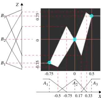
The interpolation graph becomes more imprecise when the fuzzy reference points define more permis-sive constraints. It amounts to modifying their sup-ports while ensuring some tuning conditions. In particular, the graph should remain connected in order to guarantee that any feasible input is associated with an output value. This means that conflict should be avoided when two rules are simultaneously fired, i.e. when x∈[x_i+1−, x_i+]. In other words, coherence condi-tions for the set of fuzzy rules should be satisfied [6]. In [7], additional conditions are exhibited so as to shape the interpolation graph. Actually, piecewise graphs based on 4-sided areas (see figure 2) can be obtained using a suitable tuning of the fuzzy closeness relation with respect to reference points.

Looking at figure 2, one may be disappointed that the fuzziness introduced in the closeness relations is no more present in the interpolation graph. The next sec-tion is devoted to the issue of introducing membership degrees in the 4-sided areas while keeping their sup-port unchanged. Such an appoach is motivated by the need to evaluate the relative merits of different possi-ble paths between the reference points.

X A₁ A₂ A₃ 0.75 0 0.5 B1 B2 B3 Z -0 .7 5 0 0 .7 5 Rules A₁→B₁ A₂→B₂ A₃→B₃ Reference points } (-0.75, 0.75) (0, 0) (0.5, 0.75) } } }

Figure 2: Quadrangle-based interpolation graph

3 Interpolative fuzzy graph

According to equation (2), it is obvious that using a crisp implication for defining the graph necessarily results into a crisp graph. Then, the most intuitive strategy for keeping memberhip degrees in the inter-polative graph consists in replacing Rescher-Gaines implication by another one. In order to be in accord-ance with the semantics of gradual rules, only residu-ated implications can be used, which means that:

a → b = 1 if a ≤ b and a → b = α if a > b (3) where α depends on the chosen implication. From equations (2) and (3), it is obvious that the core of the graph Γ (white areas in figure 2) does not depend on the chosen implication. Actually, only values outside the core area (black areas with zero membership gra-de in figure 2) are concerned with the implication choice. Thus, our aim when introducing membership degrees in the 4-sided areas cannot be achieved sim-ply by choosing a suitable fuzzy implication. As an al-ternative, an approach based on level 2 gradual rules (still implemented using Rescher Gaines implication) is proposed.

3.1 Nested graph family

According to section 2, it is clear that given a set of rules, i.e. a set of reference points, a collection of crisp graphs is obtained by varying the support parameters of the A_i’s and/or the B_i’s. Moreover, inclusion

prop-erties between the built graphs can be exhibited for controlling the variation of the supports as expressed by the following statements.

P1: If A_i⊆ A_i*, i=1, ..., n, then Γ*

⊆

Γ,

where Γ and Γ* are the graphs associated with rules A_i → B_i and A_i* → B_i respectively.

The proof of P1 is immediate. Indeed, (x, z) ∈ Γ* means that ∀i, A_i*(x) ≤ B_i(z). According to the as-sumption that ∀i, A_i⊆ A_i*, it follows that ∀i, A_i(x) ≤ B_i(z) which results in (x, z) ∈ Γ.

P2: If B_i* ⊆ B_i, i=1, ..., n, then Γ*

⊆

Γ,

where Γ and Γ* are now the graphs associated with rules A_i → B_i and A_i → B_i* respectively. The proof of P2 is also immediate. Indeed, (x, z) ∈ Γ* if and only if ∀i, A_i(x) ≤ B_i*(z). Since ∀i, B_i* ⊆ B_i, it follows that ∀i, A_i(x) ≤ B_i(z), i.e. (x, z) ∈ Γ.

The combination of P1 and P2 leads to:

P3: If A_i⊆ A_i* and B_i*⊆ B_i, i=1, ..., n, then Γ*

⊆

Γ, where Γ and Γ* are the graphs associated with rules A_i→ B_i and A_i*→ B_i* respectively.

Thus, according to the above inclusion properties, it is possible to design a family of nested graphs simply by building collections of nested fuzzy subsets on X and Z. Indeed, denote {A_iλ, λ∈[0,1]} a family of fuzzy subsets on X such that A_iλ’ ⊆ A_iλ if λ≥λ’ and {B_iλ,

λ∈[0,1]} a family of fuzzy subsets on Z such that B_iλ

⊆ B_iλ’ if λ≥λ’. The graph family associated with rules A_iλ→ B_iλ,λ∈[0,1], guarantees that Γλ

⊆

Γλ’ if λ≥λ’. Actually, such a construction of nested graphs simply expresses that implicative graphs increase in the sense of inclusion when underlying constraints become more permissive. Indeed, more permissive rules are obtained either by restricting input conditions further, or by enlarging output fuzzy sets.

Using a convex linear combination of fuzzy intervals enables the automatic construction of a collection of nested fuzzy subsets ranging from the lower bound of the family to the upper one. Applying such a tech-nique results in the following equation:

A_iλ = (1−λ)A_i0⊕λA_i1, λ∈[0,1], i=1, .. ,n (4) where A_i0 and A_i1, such that A_i0⊆ A_i1, are the lower and upper bounds of the family and ⊕ denotes the ex-tended sum of fuzzy numbers.

In the same way, nested output fuzzy subsets can be built according to:

} } } X A₁ A₂ A₃ B₁ B₂ B₃ Z -0.75 0.17 0.33 -0.5 -0.75 0 0.5 -0 .75 0 0. 75

B_iλ = (1−λ)B_i0⊕λB_i1, λ∈[0,1], i=1, .. ,n (5) where B_i0 and B_i1, such that B_i1⊆ B_i0 , are the upper and lower bounds of the family. It should be noted that the inclusion ordering of the B_iλ for increasing λ is the converse of the one of the A_iλ, due to opposite behav-iors with respect to graph inclusion.

Using such fuzzy subset families (see figure 3) results in the following graph inclusions:

Γ1

⊆

Γλ

⊆

Γλ’

⊆

_Γ0_{, λ,λ’ ∈[0,1] and λ≥λ’. (6)}

Figure 3: Nested fuzzy subsets (λ>λ’) Another interesting point is that the 4-sided shape is shared by all nested graphs provided that the lower and upper graphs are themselves quadrangle-shaped. 3.2 Fuzzy graph

According to the previous section, the construction of indexed nested graphs can be easily handled from the knowledge of lower and upper graphs. Now, given the above family {Γλ, λ∈[0,1]}, there is a unique fuzzy set F whose λ−cuts F_λ are precisely Γλ for each λ

∈[0,1]. This fuzzy set is built using the standard rep-resentation theorem [11], that is:

µ_F(x, z) = sup_{λ ∈[0,1]} min (λ, Γλ(x, z) ) (7) It should be noticed that equation (7) is based on the equality F_λ = Γλ in which two different meanings of

λ are involved depending on the used notation. When

λ is used as a subscript, it should be interpreted as a level-cut. On the other hand, the corresponding super-script is relative to the index of an element of a family of nested subsets.

According to formulation (7), the reconstructed F is finally a classical fuzzy graph defined on X x Z. An-other interpretation consists in viewing F as a fuzzy set of crisp graphs, that is as a level 2 fuzzy set [12]. In this case, F is represented as:

F =

∫

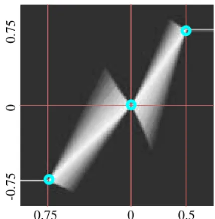
_{λ ∈[0,1]}λ / Γλ (8) according to Zadeh’s notation where the integral sign stands for the union of the fuzzy singletons λ / Γλ.

Figure 4 plots the fuzzy graph obtained when the low-er graph Γ1 is precise and piecewise linear (as in fig-ure 1) and the upper graph Γ0has the quadrangle-based shape of figure 2.

Figure 4: Fuzzy graph obtained by a set of gradual rules

According to Figure 3, families {A_iλ, λ∈[0,1]} and

{B_iλ, λ∈[0,1]}, i=1, ...,n, can also be viewed as type 2 fuzzy subsets, i.e. fuzzy sets with fuzzy membership grades [12]. In this framework, one may wonder if ex-tending the Rescher-Gaines implication to fuzzy set-valued arguments would be compatible with equation (7). Let us examine this approach a little further in the case of a single rule, i.e. n=1.

Let and be type 2 fuzzy subsets on X and Z de-fined according to nested families {Aλ, λ∈[0,1]} and

{Bλ, λ∈[0,1]}.

It follows that membership degrees in and are now fuzzy subsets on [0,1], that is:

and , (9)

where the membership functions of and can be deduced from the construction of and . When x and z belong to the support of A0 and B1, the mem-bership functions obtained for and are given in Figure 5.

Figure 5: Fuzzy membership degrees and Let f be the Rescher-Gaines implication, that is the A_i0 A_i1 A_iλ_A' iλ X 1 B_i1 B_i0 B_iλ_B iλ' Z 1 } } } 0.75 0 0.5 -0 .7 5 0 0. 75 A˜ B˜ A˜ B˜ µ A˜( )x = a˜ x( ) µB˜( )z = b˜ z( ) a˜ x( ) b˜ z( ) A˜ B˜ a˜ x( ) b˜ z( ) t 0 µ_A0(x) µA1(x)1 λ 1 µ_Aλ(x) t 0 µ_B1(z) µB0(z) 1 µ_Bλ(z) λ 1 a˜ x( ) b˜ z( ) a˜ x( ) b˜ z( )

mapping from [0,1]x[0,1] to {0,1} defined by f(a,b) = a→b. Extending f to the fuzzy set-valued arguments

and leads to:

= sup{λ∈[0,1]: t∈f( _λ, _λ)}(10) where t∈{0,1} and _λ (resp. _λ) denotes the λ− cut of (resp. ). Since _λ = [µ_Aλ(x), µ_A1(x)] and _λ = [µ_B1(z), µ_Bλ(z)] (see Figure 5), it follows that:

(1) = sup{λ∈[0,1]: µ_Aλ(x)≤ µ_Bλ(z)}(11) and

(0) = 1 if µ_A1(x) > µ_B1(z) (12)

= 0 otherwise. (13)

From equations (11) and (7), it can be concluded that:

µ_F(x, z) = (1) (14)

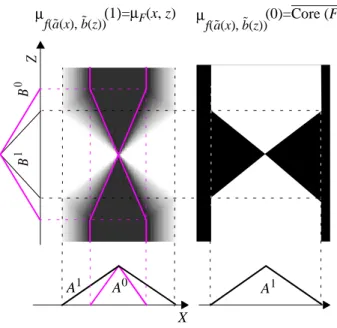
which means that the fuzzy graph F can be obtained from a type 2 reasoning by considering the “true” case only. The information provided by the “false” case is quite poorer since the degree of membership of 0 to f( , ) simply defines the complement of the core of F, i.e. this degree is 1 if (x, z) ∉ core(F) and 0 otherwise.

Links between type 2 and level 2 interpretations are illustrated on figure 6 for a single gradual rule.

Figure 6: Type 2-based construction

Further computations are still necessary for combing several implicative rules in the case of a type 2 in-terpretation. Actually, even if both approaches (level

2 and type 2 constructions) lead to similar fuzzy graphs, it is more convenient to adopt the level 2 in-terpretation.

The proposed approach based on (7) or (14) provides a constructive method for deriving a genuine fuzzy implication from a set of gradual rules. That it is a genuine implication can be checked by verifying the following properties: if µ_A1(x) ≥µ_A1(x*) then µ_F(x, z) ≤µ_F(x*, z) if µ_B0(z) ≥µ_B0(z*) then µ_F(x, z) ≥µ_F(x, z*) Moreover, if µ_A1(x) = 1 then µ_F(x, z) = 0 when µ_B0(z) ≠1 if µ_A1(x) = 0 then µ_F(x, z) = 1

if µ_B0(z)= 1 then µ_F(x, z) = 1 (identity principle). It is interesting to compare our construction to the one in [4]. This paper establishes results under which fuzzy implications can be decomposed as convex sums of crisp rules. It assumes a finite number of membership grades. Under certain mild conditions, this decomposition involves a nested family of gradu-al rules of the form m_i(A)→B where {m_i} is a family of modifiers affecting the condition part only. In the present paper, both conditions and conclusions are varied.

4 Conclusion

This paper illustrates how fuzzy interpolation graphs can be obtained from gradual rules. The easiest strat-egy consists in building nested crisp graphs whose weighting allows the construction of the final fuzzy graph in the form of a level 2 graph.

This method is compatible with a type 2 interpretation which applies the extension principle to the Rescher-Gaines implication with fuzzy set-valued arguments. An interesting point for further investigation concerns the interpretation of the interpolative crisp graphs in terms of some properties of the underlying functions, especially their derivatives. If such links could be ex-hibited, they would provide a theoretical framework for the choice of the lower and upper graphs that are used for the building of the fuzzy interpolative graphs.

From a practical point of view, a relevant use of the proposed fuzzy interpolation technique still requires that the multi-input case be developed. In this context, the construction of nested interpolation graphs by means of families of gradual rules with composite an-a˜ x( ) b˜ z( ) µ f a˜ x( ( ) b˜ z, ( ))( )t a˜ x( ) b˜ z( ) a˜ x( ) b˜ z( ) a˜ x( ) b˜ z( ) a˜ x( ) b˜ z( ) µ f a˜ x( ( ) b˜ z, ( )) µ f a˜ x( ( ) b˜ z, ( )) µ f a˜ x( ( ) b˜ z, ( )) a˜ x( ) b˜ z( ) X A0 A1 Z B 1 B 0 A1 (1)=µ_F(x, z) _µ f a˜ x( ( ) b˜ z, ( ))(0)=Core (F) µ f a˜ x( ( ) b˜ z, ( ))

tecedents is also a matter of further research.

References

[1] Anile A.M., Falcidieno B., Gallo G., Spagnuolo M., Spinello S., “Modeling uncertain data with fuzzy B-splines”, Fuzzy Sets and Systems, Vol. 113, pp. 397-410, 2000.

[2] D. Dubois, F. Esteva, P. Garcia, L. Godo, H. Pra-de, “A logical approach to interpolation based on similarity relations”, Int. J. of Approximate Reasoning, Vol. 17, no. 1, pp. 1-36, 1997. [3] D. Dubois, F. Esteva, P. Garcia, L. Godo, R.L. de

Mantaras, H. Prade, “Fuzzy set modelling in case-based reasoning”, Int. J. of Intelligent Sys-tems, Vol. 13, no 4, pp. 345-373, 1998.

[4] D. Dubois, E. Hüllermeier, H. Prade, “On the re-presentation of fuzzy rules in terms of crisp ru-les”, Information Sciences, Vol. 151, pp. 301-326, 2003.

[5] D. Dubois, H. Prade, “Gradual inference rules in approximate reasoning”, Information Sciences, Vol. 61, no 1-2, pp. 103-122, 1992.

[6] Dubois D., Prade H., Ughetto L., “Checking the Coherence and Redundancy of Fuzzy Knowled-ge Bases”, IEEE Trans. on Fuzzy Systems, Vol. 5, no 3, pp. 398-417, Aug. 97.

[7] Galichet S., Dubois D., Prade H., “Imprecise spe-cification of ill-known functions using gradual rules”, Proc. of the 2nd Int. Workshop on Hybrid Methods for Adaptive Systems (EUNITE’02), Albufeira, Portugal, pp. 512-520, Sept. 2002. [8] Galichet S., Dubois D., Prade H., “Imprecise

mo-delling using gradual rules and its application to the classification of time series”, Proc. of the 10th IFSA World Congress (IFSA2003), Is-tanbul, Turkey, June 2003.

[9] Kaleva O., “Interpolation of fuzzy data”, Fuzzy Sets and Systems, Vol. 61, pp. 63-70, 1994. [10] Lowen R., “A fuzzy Lagrange interpolation

theo-rem”, Fuzzy Sets and Systems, Vol. 34, pp. 33-38, 1990.

[11] Zadeh L. , “Fuzzy sets”, Information Control, Vol. 8, pp. 338-353, 1965.

[12] Zadeh L. , “Quantitative fuzzy semantics”, Infor-mation Sciences, Vol. 3, no 2, pp. 159-176, 1971.