Experimental Study of Choking Flow of Water at Supercritical Conditions

(1)

UNIVERSITÉ DE MONTRÉAL

EXPERIMENTAL STUDY OF CHOKING FLOW OF WATER AT

SUPERCRITICAL CONDITIONS

ALTAN MUFTUOGLU

DÉPARTEMENT DE GÉNIE PHYSIQUE ÉCOLE POLYTECHNIQUE DE MONTRÉAL

THÈSE PRÉSENTÉE EN VUE DE L’OBTENTION DU DIPLÔME DE PHILOSOPHIÆ DOCTOR

(GÉNIE NUCLÉAIRE) MAI 2014

(2)

UNIVERSITÉ DE MONTRÉAL

ÉCOLE POLYTECHNIQUE DE MONTRÉAL

Cette thèse intitulée:

EXPERIMENTAL STUDY OF CHOKING FLOW OF WATER AT SUPERCRITICAL CONDITIONS

présentée par : MUFTUOGLU Altan

en vue de l’obtention du diplôme de : Philosophiæ Doctor a été dûment acceptée par le jury d’examen constitué de : M. KOCLAS Jean, Ph. D., président

M. TEYSSEDOU Alberto, Ph. D., membre et directeur de recherche M. BALAZINSKI Marek, Docteur ès sciences, membre

(3)

DEDICATION

(4)

ACKNOWLEDGMENTS

It is impossible to acknowledge all the individuals who helped me during this study; the following individuals are specifically appreciated.

Foremost, I would like to express my sincere gratitude to Professor Alberto Teyssedou, my director, for his guidance throughout this project. His ceaseless energy, inventiveness and insightful criticism guided me to complete a rigorous work. Without his experience and patience, it would be impossible to complete this research program.

I would like to take this opportunity to thank Professor Altan Tapucu, for his excellent guidance and encouragement throughout my time in Ph.D. program at École Polytechnique de Montreal. I have benefited greatly from his generosity and expertise.

I also would like to thank Professor Andrei Olekhnovitch, my former co-supervisor, for his help getting me started in thermal-hydraulics laboratory.

I owe special gratitude to all the members of nuclear engineering institute, fellow graduate students and friends. The participation of Thierry Lafrance (Ing.), Stephen Schneller (Ing.), Cyril Koclas (Associate Researcher) and Jean-Claude Juneau (Technician) are greatly appreciated. Without them the realization of this research program should be impossible. The recognition and continuous support of Dr. Laurence Leung from AECL is largely appreciated.

I also would like to thank all jury members, Professor Glenn Harvel, Professor Jean Koclas, Professor Marek Balazinski and Professor Saydy Lahcen for their support and helpful suggestions.

Finally, I would like to thank my parents for providing me unconditional support. Special thanks are due to my wife for her support, patience, love and understanding throughout the several years of my doctoral work.

The work presented in this thesis was possible due to the financial support of the Gen-IV CRD research program granted by the Natural Sciences and Engineering Research Council of Canada (NSERC), National Resources Canada, Atomic Energy of Canada Limited, Hydro-Québec and Alexander Graham Bell Canada Graduate Scholarship granted by NSERC.

(5)

RÉSUMÉ

Les prochaines générations de réacteurs nucléaires vont opérer avec un fluide de refroidissement dont la pression sera près de 25 MPa et dont la température de sortie sera de 500°C à 625°C, selon le type de réacteur. En conséquence, l’enthalpie du flux de sortie de ces futurs réacteurs à eau supercritique, SCWR, «Supercritical Water-Cooled Reactors» sera beaucoup plus élevée que celle des réacteurs actuels. Cela permettra à l’efficacité des centrales nucléaires de passer d’environ 30-33% aujourd’hui jusqu’à 48%. Cependant, le comportement thermo-hydraulique de l’eau supercritique n’est pas encore bien compris sous de telles conditions d’écoulement, notamment en ce qui concerne par exemple les chutes de pression, la convection forcée, la détérioration du transfert de chaleur et le flux massique critique. Jusqu’à maintenant, seul un nombre très limité de recherches ont été effectuées utilisant des fluides en conditions supercritiques. De plus, ces recherches n’ont pas été effectuées dans des conditions représentatives des SCWR. Aussi, les données existantes au sujet du flux massique critique ont été recueillies lors d’expériences dont la pression de décharge était celle de l’atmosphère ambiante, et dans la plupart des cas en utilisant des fluides autres que l’eau. Il est à noter que la compréhension de l’écoulement critique des fluides supercritiques est essentielle pour effectuer les analyses de sûreté des futurs réacteurs nucléaires et pour concevoir leurs principaux composants mécaniques, par exemple, les valves de contrôle et les vannes de sûreté. Ainsi donc, une installation d’eau supercritique a été construite à l’École Polytechnique de Montréal pour effectuer des recherches sur le débit critique. Ce montage expérimental consiste en deux boucles fonctionnant en parallèle, servant à déterminer les conditions d’écoulement qui déclenchent le débit critique de l’eau supercritique. Cette installation est également en mesure d’effectuer des expériences de transfert de chaleur et de perte de pression utilisant de l’eau en conditions supercritiques.

Dans cette thèse, seront présentés les résultats obtenus grâce à cette installation avec l’utilisation d’une section d’essais munie d’un orifice de 1 mm de diamètre interne et de 3,17 mm de longueur, et dont les rebords sont acérés. Ainsi, 545 points de données de flux massique critique ont été obtenus en conditions supercritiques, pour des pressions d’écoulement allant de 22,1 MPa à 32,1MPa, et à des températures d’écoulement allant de 50°C à 502°C, et ce pour des pressions

(6)

de décharges 0,1 MPa à 3,6 MPa. Les données obtenues sont comparées avec celles provenant de la littérature pour l’eau et même pour le dioxyde de carbone en conditions supercritiques.

Il est également très important de mentionner que les modèles actuels utilisés pour prédire les flux massiques critiques ont été développés pour des fluides en conditions sous-critiques. Même si aucun de ces modèles n'a été développé spécifiquement pour gérer l'expansion des fluides supercritiques, les prédictions des quelques-uns de ces modèles ont été comparées avec les données obtenues expérimentalement en conditions supercritiques. De plus, un simple modèle polytropique est proposé pour estimer les flux massiques critiques. Les résultats de cette comparaison aideront les concepteurs des futurs réacteurs à choisir correctement les dispositifs de sécurité nucléaire.

Dans la littérature, la différence entre la température du fluide et la valeur de la température pseudo-critique (DTpc) est utilisée pour traiter les données de débit massique critique. À cette fin,

il doit être mentionné qu’une nouvelle relation est proposée pour estimer les températures pseudo-critiques de l’eau et du dioxyde de carbone. En particulier, pour des températures d’écoulement moindres que leurs valeurs pseudo-critiques, les flux critiques semblent se produire dans une région très limitée. Près de la température pseudo-critique, nos expériences fournissent des données dans une région où les données des recherches antérieures ont été très rares.

En général, un excellent accord est observé avec les expériences effectuées par d'autres chercheurs, mais avec une précision supérieure. Le flux massique diminue alors que la température en amont de l’orifice augmente. En particulier, le montage expérimental permet de contrôler les paramètres d’opération avec perfection. En outre, un faible gradient de pression se produisant en amont de l’orifice est systématiquement mesuré. Il est aussi observé que près de la température pseudo-critique, le coefficient de transfert de chaleur change très rapidement, ce qui affecte la différence entre la température de la surface intérieure du tube et celle du liquide de refroidissement. Ces variations rapides associées à la variation correspondante de la densité du fluide rendent très difficile le contrôle et le maintien des conditions d’écoulement à proximité de l’état critique.

On a trouvé que le facteur dominant sur le débit massique critique est la température en amont de l’orifice. L’augmentation de cette température entraine toujours la diminution du débit massique. Pour des températures bien inférieures à la température critique (ou de la température

(7)

pseudo-critique si la pression est différente de la pression pseudo-critique), le taux de cette diminution est faible. Toutefois, lorsque la température du fluide en amont se rapproche de la température critique, le taux de la diminution du débit massique augmente significativement en raison de la baisse drastique de la densité du fluide. Après avoir dépassé la température critique, la densité du fluide change lentement et donc le taux de diminution du débit massique redevient faible. Enfin, en utilisant des prédictions obtenues par les modelés HEM «Homogeneous Equilibrium Model», M-HEM «Modified-Homogeneous Equilibrium Model», par l'équation de Bernoulli, ainsi que par l'équation polytropique, les prédictions de ces modèles sont comparées avec les données expérimentales. En général, pour les écoulements dans des conditions de températures sous-critiques, on observe que l'équation de Bernoulli avec coefficient de débit de 0,7 est satisfaisante pour prédire l'évolution expérimentale. D'autre part, à des températures supercritiques et autour des températures pseudo-critiques, M-HEM est le plus approprié pour prédire les débits massiques. Cependant, l'équation de Bernoulli peut aussi être utilisée dans une certaine mesure avec un coefficient de débit de 0,4 pour les températures supercritiques et de 0,7 pour les températures sous-critiques.

Le projet présenté dans cette thèse a fait l’objet de deux présentations lors de conférences internationales, d’une séance d’affichage et d’une publication dans un journal scientifique.

 A. Muftuoglu and A. Teyssedou, Design of a supercritical choking flow facility, UNENE R&D Workshop 2011, Toronto, Ontario, Canada, 12-13 December 2011.

 A. Hidouche, A. Muftuoglu and A. Teyssedou, Comparative study of different flow models used to predict critical flow conditions of supercritical fluids, The 5th International Symposium of SCWR (ISSCWR-5), Vancouver, British Columbia, Canada, March 13-16, 2011.

 A. Muftuoglu and A. Teyssedou, Experimental study of water flow at supercritical pressures, 34th Annual Conference of Canadian Nuclear Society/ 37th Annual CNS/CNA Student Conference, Toronto, Ontario, Canada, 9-12 June 2013.

 A. Muftuoglu and A. Teyssedou, Experimental Study of Abrupt Discharge of Water at Supercritical Conditions, Experimental Thermal and Fluid Science, Volume 55, February 2014, Pages 12-20.

(8)

ABSTRACT

Future nuclear reactors will operate at a coolant pressure close to 25 MPa and at outlet temperatures ranging from 500oC to 625°C. As a result, the outlet flow enthalpy in future

Supercritical Water-Cooled Reactors (SCWR) will be much higher than those of actual ones which can increase overall nuclear plant efficiencies up to 48%. However, under such flow conditions, the thermal-hydraulic behavior of supercritical water is not fully known, e.g., pressure drop, forced convection and heat transfer deterioration, critical and blowdown flow rate, etc. Up to now, only a very limited number of studies have been performed under supercritical conditions. Moreover, these studies are conducted at conditions that are not representative of future SCWRs. In addition, existing choked flow data have been collected from experiments at atmospheric discharge pressure conditions and in most cases by using working fluids different than water which constrain researchers to analyze the data correctly. In particular, the knowledge of critical (choked) discharge of supercritical fluids is mandatory to perform nuclear reactor safety analyses and to design key mechanical components (e.g., control and safety relief valves, etc.). Hence, an experimental supercritical water facility has been built at École Polytechnique de Montréal which allows researchers to perform choking flow experiments under supercritical conditions. The facility can also be used to carry out heat transfer and pressure drop experiments under supercritical conditions. In this thesis, we present the results obtained at this facility using a test section that contains a 1 mm inside diameter, 3.17 mm long orifice plate with sharp edges. Thus, 545 choking flow of water data points are obtained under supercritical conditions for flow pressures ranging from 22.1 MPa to 32.1 MPa, flow temperatures ranging from 50°C to 502°C and for discharge pressures from 0.1 MPa to 3.6 MPa. Obtained data are compared with the data given in the literature including those collected with fluids other than water.

It is also important to mention that present models used to predict supercritical choking flows have been developed for fluids under subcritical conditions. Even though none of these models were developed to handle the expansion of supercritical fluids, we tested some of the models (Homogenous Equilibrium Model, Modified-Homogeneous Equilibrium Model and Bernoulli equation) under supercritical conditions and compared their predictions with our data and those of other researchers, available in the literature. In addition, a simple polytropic model is proposed to estimate the critical flow rate of water. It is found that the Modified Homogeneous Equilibrium

(9)

Model is the most appropriate model to estimate the discharge flow rate of water under supercritical conditions. Results of the model comparison must help SCWR designer to choose safety devices correctly.

As a common practice, the difference between the fluid temperatures with respect to the pseudo-critical value (DTpc) is used to treat the data. To this aim, it must be mentioned that a new relationship is proposed to estimate the pseudo-critical temperature of water and carbon dioxide. In particular, for flow temperatures lower than pseudo-critical values, choking flow seems to occur within a very limited region. Close to the pseudo-critical temperature, our experiments provide data in a region where up to now, are very scarce.

In general, an excellent agreement with experiments carried out by other researchers is obtained. It is observed that the mass flux decreases with increasing the flow temperature upstream of the orifice. In particular, the proposed experimental arrangement (i.e., use of two loops running in parallel) permitted us to determine flow conditions that trigger supercritical water choking flow. Furthermore, a small pressure gradient occurring upstream of the orifice is systematically measured. It is also observed that close to the pseudo-critical point, the heat transfer coefficient changes very rapidly which affects the difference between the inner tube surface and coolant temperatures. These fast variations combined with the corresponding change in fluid density make it very difficult to control and maintain flow conditions in the proximity of the critical point.

The research work presented in this thesis has been the subject of two presentations at international conferences, a poster session and a publication in a scientific journal.

(10)

(11)

LIST OF TABLES

Table 1.1 Critical parameters of fluids [5]. ... 20

Table 1.2 Nozzle dimensions and shapes used by Lee and Swinnerton [96]. ... 45

Table 1.3 Nozzle dimensions and geometries used by Mignot et al. [104]. ... 49

Table 2.1 Medium pressure loop operational limits. ... 54

Table 2.2 Supercritical pressure loop operational limits. ... 56

Table 2.3 Preliminary electrical calculations of each heater element branchat106V. ... 68

Table 2.4 Comparison of estimated pressure drop vs. measured pressure drop between the calming chamber and the test section. ... 72

Table 2.5 Estimated pressure drop in the heater element. ... 73

Table 2.6 Technical information of the pressure transducers used on the test section. ... 92

Table 2.7 Technical information of the NI modules used on DAS. ... 101

Table 3.1 Experimental matrix. ... 104

Table 3.2 Experimental conditions. ... 106

Table 4.1 Experimental matrix. ... 139

Table 4.2 Precision of measurements in three different experimental regions. ... 139

Table 5.1 Experimental fluid states shown in Figure 5.1. ... 142

Table 5.2 Experimental matrix used to obtain complementary results. ... 143

Table 5.3 Experimental errors for each flow regions shown in Figure 5.12. ... 156

Table 5.4 Results for two similar experiments performed on different days. ... 159

(16)

LIST OF FIGURES

Figure 1.1 Schematic of round edged nozzle. ... 8

Figure 1.2 Mass flux (G) as a function of pressure ratio (Pd / Po). ... 9

Figure 1.3 Pressure distribution in the nozzle for different back pressure values. ... 9

Figure 1.4 Speed of sound vs. temperature at constant pressures. ... 12

Figure 1.5 Pressure-temperature phase diagram for water. ... 13

Figure 1.6 Specific heat capacity vs. fluid temperature for different constant pressures. ... 15

Figure 1.7 Change of speed of sound as a function of temperature. ... 16

Figure 1.8 Change of density as a function of temperature. ... 16

Figure 1.9 Change of enthalpy as a function of temperature. ... 17

Figure 1.10 Change of viscosity as a function of temperature. ... 17

Figure 1.11 Change of specific isobaric heat capacity as a function of temperature. ... 18

Figure 1.12 Change of specific isochoric heat capacity as a function of temperature. ... 18

Figure 1.13 Specific heat ratio as a function of temperature. ... 19

Figure 1.14 Pressure-temperature diagram for water and liquid-like and gas-like supercritical regions. ... 21

Figure 1.15 Blowdown map of water’s depressurization from supercritical conditions. ... 47

Figure 2.1 Medium pressure steam-water thermal loop. ... 54

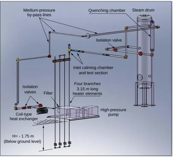
Figure 2.2 The supercritical water experimental facility. ... 56

Figure 2.3 Isometric view of the supercritical part of the loop. ... 57

Figure 2.4 Heater element with electrical connections. ... 61

Figure 2.5 Silver foil between heater tubes and copper clamps. ... 61

Figure 2.6 Heater element with Superwool insulation. ... 62

(17)

Figure 2.8 Schematic of a bended tube used to perform mechanical analyses. ... 64

Figure 2.9 Bending analysis of a Hastelloy C-276 0.065" thick tube. ... 65

Figure 2.10 Estimated temperature distributions along the heater tube. ... 69

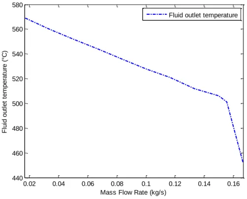
Figure 2.11 Fluid outlet temperature as a function of heater mass flow rate. ... 70

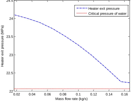
Figure 2.12 Heater exit pressure as a function of mass flow rate. ... 74

Figure 2.13 Calming chamber. ... 75

Figure 2.14 Test section with sharp edged orifice. ... 76

Figure 2.15 Photo of the test section showing the welded region. ... 77

Figure 2.16 Isenthalpic and isentropic expansions from supercritical state. ... 78

Figure 2.17 Quenching chamber. ... 81

Figure 2.18 Location of spot welded thermocouples on the heater element. ... 83

Figure 2.19 A typical spot welded thermocouple on the heater element external surface. ... 84

Figure 2.20 Distance measurement between a thermocouple and the copper bus bar. ... 85

Figure 2.21 Cross-sectional view of the heater element assembly. ... 86

Figure 2.22 Installation procedure of radially positioned thermocouples. ... 87

Figure 2.23 Installation procedure of radially positioned thermocouples – application of a chemical cement (Omegabond® 600) fixation layer. ... 87

Figure 2.24 Partial view of the temperature measurement panel and the galvanic isolator amplifiers. ... 88

Figure 2.25 Typical calibration of type-K thermocouples used in the heater element. ... 89

Figure 2.26 Typical responses of the entire temperature measurement chain including thermocouples, wires, galvanic isolation amplifiers and data acquisition system. ... 90

Figure 2.27 Typical calibration data obtained for a Thermowell. ... 91

Figure 2.28 Location of pressure taps and pressure lines (in red) used to perform choking flow experiments. ... 93

(18)

Figure 2.29 Responses of medium pressure transducers. ... 94

Figure 2.30 Flowmeter (FTr-2) response. ... 96

Figure 2.31 Power measurement and control station. ... 97

Figure 2.32 Electrical current measurement devices. ... 98

Figure 2.33 Carbon filament light bulb system to commission the electrical power. ... 99

Figure 2.34 Data acquisition system. ... 100

Figure 2.35 Process variables screen shot. ... 101

Figure 2.36 Control variables screen shot. ... 102

Figure 2.37 Variable charts screen shot. ... 102

Figure 3.1 Two loops running in parallel. ... 103

Figure 3.2 Typical change of upstream thermo-physical conditions for blowdown type of experiments. ... 105

Figure 4.1 Portion of the supercritical-water experimental facility. ... 128

Figure 4.2 Commissioning tests of a damper unit. ... 129

Figure 4.3 Test section with 1 mm orifice plate and pressure taps. ... 130

Figure 4.4 Comparison of results obtained with a new pseudo-critical temperature correlation. 131 Figure 4.5 École Polytechnique supercritical water data. ... 132

Figure 4.6 Comparison of École Polytechnique data with those given in the literature. ... 133

Figure 4.7 Comparison of École Polytechnique data with CO2 data from Mignot et al. [4,7,9]. 134 Figure 4.8 a) Pressure distribution along the test section vs. discharge pressure, b) Mass flux vs. discharge pressure at different temperatures. ... 135

Figure 4.9 Variations of density and speed of sound for water at supercritical pressure. ... 136

Figure 4.10 Experimental data represented on the T-S diagram. ... 137

Figure 4.11 Precision of the measurements for Region I (DTpc < -50oC in Figure 4.5.) ... 138

(19)

Figure 5.2 Mass flux as a function of DTpc. ... 142

Figure 5.3 a) Isentropic flow expansion, b) Isenthalpic flow expansion. ... 144

Figure 5.4 Isentropic expansion coefficient for different upstream flow pressures at 450°C. ... 147

Figure 5.5 Isentropic expansion coefficient for different upstream flow pressures at 500°C. ... 148

Figure 5.6 Comparison of HEM and M-HEM (C = 0.6) with experimental data at Po=24 MPa.148 Figure 5.7 Comparison of M-HEM (C = 0.8) with experimental data at Po=24 MPa. ... 149

Figure 5.8 Comparison of the prediction obtained Bernoulli’s equation with experimental data at Po=24 MPa; Pd=0.8 MPa. ... 150

Figure 5.9 Comparison of the prediction obtained with the polytropic equation with experimental data for  =1.30, Po=24 MPa. ... 151

Figure 5.10 Averaged data vs. continuous data collection at supercritical pressures. ... 153

Figure 5.11 Evolution of experimental parameters for continuous data collection. ... 154

Figure 5.12 Repeatability study. ... 155

Figure 5.13 Mass flux as a function of DTpc and discharge pressure at 23 MPa. ... 157

Figure 5.14 Radial temperature at the exit of the heater element. ... 159

Figure 5.15 Heater element measured surface temperatures. ... 160

Figure 5.16 Estimated heat transfer coefficient using the Dittus-Boelter equation. ... 164

Figure 5.17 Heat transfer coefficient as a function of bulk fluid temperature. ... 165

Figure 5.18 Temperature profile along the heater element. ... 166

Figure 5.19 Estimated heat transfer coefficient for different flow pressure conditions. ... 168

Figure 6.1 Data acquisition and control-1. ... 202

Figure 6.2 Data acquisition and control-2. ... 203

(20)

LIST OF SYMBOLS AND ABBREVIATIONS

Symbols

a Wave velocity (m/s)

A Cross sectional flow area (m2)

C Sound velocity (m/s)

Cd Discharge coefficient

cp Specific heat at constant pressure (kJ/kg.K)

cv Specific heat at constant volume (kJ/kg.K)

DTpc Temperature difference between the fluid with respect to the pseudo-critical value

FTr Flow rate transmitter (L/s) g Gravity (m/s2)

G Mass flux (kg/m2.s)

Gr Grashof number

h Convective heat transfer coefficient (W/m2.K)

I Current (A)

k Specific heat ratio, thermal conductivity (W/m.K) L Characteristic length (m)

m Mass flow rate (kg/s)

Ma Mach number

Nu Nusselt number

P Pressure (MPa)

Pr Prandtl number

PTr Pressure transducer (MPa)

(21)

R Electrical resistance ()

Re Reynolds number

s Entropy (kJ/kg.K)

T Temperature (°C)

TTr Temperature transducer (°C) u Average flow velocity (m/s)

 Specific volume (m3/kg) V Fluid velocity (m/s)

x Thermodynamic quality

ΔG Mass flux difference (kg/m2.s)

Δh Enthalpy difference (kJ/kg), elevation difference (m) Δs Entropy difference (kJ/kg.K)

 Void fraction coefficient

 Surface roughness (m)

 Isentropic expansion coefficient

 Specific mass (kg/m3), electrical resistivity (Ω⋅m)

 Pressure drop coefficient

 Correction factor

Subscripts and superscripts

acc acceleration

amb ambient

o stagnation

b bulk fluid

(22)

C sonic d discharge el electrical E equilibrium f fluid fr friction g gas grav gravitation in inlet l liquid

n polytropic expansion coefficient

pc pseudo-critical

r ratio

sur surface

t throat (critical plane)

tp triple point

x reference temperature

Abbreviations and acronyms

AECL Atomic Energy of Canada Limited

AO Analog Output

ASME American Society of Mechanical Engineers

BV Block Valve

BWR Boiling Water Reactor CANDU Canada Deuterium Uranium

(23)

CHF Critical Heat Flux

CV Control Valve

DAS Data Acquisition System

DC Direct Current

EDM Electro Discharge Method FFPP Fossil Fuel Power Plant

FM Frequency Modulated

FPGA Field-Programmable Gate Array GIF Generation International Forum GFR Gas-Cooled Fast Reactor System HEM Homogeneous Equilibrium Model

HP High Pressure

ID Inside Diameter

IEA International Energy Agency

I/O Input/output

LFR Lead-Cooled Fast Reactor System LOCA Loss of Coolant Accident

LPF Low Pass Filter

M-HEM Modified Homogeneous Equilibrium Model MSR Molten Salt Reactor System

NI National Instrument

NIST National Institute of Standards and Technology NPP Nuclear Power Plant

(24)

OD Outside Diameter

PWR Pressurized Water Reactor RBQ Régie du Bâtiment du Québec R&D Research and Development RMS Root Mean Square

RPM Revolutions Per Minute

SCH Schedule

SCR Silicon Controlled Rectifier

SCWR Supercritical Water-Cooled Reactor SFR Sodium-Cooled Fast Reactor System

SS Stainless Steel

VHTR Very-High-Temperature Reactor System

(25)

LIST OF APPENDIXES

Appendix 1 – Certification of the RBQ ………..…….…188 Appendix 2 – Pressure transducer calibrations………...………...191 Appendix 3 – Control valve calibrations……….……...201 Appendix 4 – Data acquisition and control program………202 Appendix 5 – Drawings of the test section……….………..205 Appendix 6 – Loop operation checklist………207

(26)

INTRODUCTION

For years, world energy needs are continuously increasing. Hence, the International Energy Agency (IEA) has stipulated that by the year 2040, world energy requirements will increase by 56% [1]. Therefore, to assure a worldwide good economic growth, as well as adequate social standards in a relatively short term, new energy-conversion technologies are mandatory. In that respect, nuclear industry may play an important role to overcome these requirements. In particular, like most of the developed countries, Canada has largely contributed in different research and development (R&D) programs that permitted the national nuclear industry to continue growing. To this aim, Canada has signed the Generation IV International Forum (GIF) agreement in July 2001 to develop new technologies for the future. Thus, GIF members have selected the development of six new generations of nuclear power reactors to replace present technologies such as: Gas-Cooled Fast Reactor System (GFR), Lead-Cooled Fast Reactor System (LFR), Molten Salt Reactor System (MSR), Sodium-Cooled Fast Reactor System (SFR), Supercritical Water-Cooled Reactor System (SCWR), Very-High-Temperature Reactor System (VHTR). The principal goals of these power reactors among others are economic competitiveness, sustainability, safety, reliability and resistance to proliferation. In addition to these advantages, these reactors must also permit other energy applications, such as hydrogen production, seawater desalination and petroleum extraction [2].

Within this framework, from these six different nuclear reactors that will be developed by GIF members, Canada has oriented the R&D towards the design of a Supercritical Water-Cooled Reactor (SCWR), which up to now is the only proposed water-cooled nuclear reactor design. According to preliminary design criteria of these concepts, future supercritical reactors will use water as coolant at severe operating conditions. The working pressure will be 25 MPa and reactor coolant inlet/outlet temperature will be around 280°C / 510°C – 625°C, respectively depending on the proposed design [3]. Since the operating pressure is higher than the critical pressure of water (22.06 MPa), boiling phenomena will not occur in SCWRs and complex two-phase problems will be significantly reduced. It is very important to mention that even though there will be no boiling in SCWRs, the density, as well as other thermo-physical properties will change rapidly close to the critical temperature of water (373.95°C). As an example, Figure I-1 shows the change of fluid density between inlet and outlet of the reactor coolant at two different pressures

(27)

covering the critical temperature zone. This figure shows that the density between the inlet and the outlet of the reactor core will change by a factor of 11.5 times even though no subcritical type boiling flow occurs. It must be mentioned that the thermo-physical properties of water presented in this study are obtained using NIST Standard Reference Database 23 [4].

Figure I.1 Change of density as a function of temperature at critical pressure and SCWR’s operating pressure.

Moreover, in future nuclear power plants, not only the chance of Critical Heat Flux (CHF) phenomena will be reduced, but also the use of single-phase flow in the reactor will eliminate several equipments, such as: pressurizers, steam generators and steam separators that are used in Pressurized Water Reactors (PWR) and Boiling Water Reactors (BWR). Also, having high outlet fluid temperatures will increase the coolant outlet enthalpy and decrease its density; therefore for a given thermal power much less coolant mass flow rate will be required. Consequently, the water inventory of SCWRs will be low and will require less pump power as compared to actual reactors which will make the reactor more compact. All these advantages, among others, will improve net thermal efficiency of the reactor up to 44-50% as compared to about 30% efficiency for existing nuclear power plants. Furthermore, compactness of the nuclear reactor including

300 350 400 450 500 550 600 0 100 200 300 400 500 600 700 800 Temperature (°C) F lu id d e n s it y ( k g /m 3) 22.1 MPa 25.0 Mpa

(28)

plant simplifications will reduce the capital cost of the reactor which is very high for nuclear power plants (NPP) comparing to other types of power plants [3].

SCWRs will be built based on a similar technology used for supercritical fossil fuel power reactors (FFP), BWRs and PWRs. BWRs, PWRs and several supercritical FFPs are already in operation since 1950s [5, 6]. This valuable engineering knowledge, combined with the actual know-how of supercritical water fossil-fired power plants, could be implemented together for designing future SCWRs. Hence, SCWR appears as the foremost candidate of future nuclear power plants to be built by the year 2040. Consequently, it is expected that in the near future, SCWR technology will replace actual Generation III or advanced Canada Deuterium Uranium (CANDU) reactors. Even though Canada has more than 56 years of experience in the construction and operation of nuclear power plants, it is obvious that designing future SCWRs will be impossible without performing extensive experimental and theoretical studies of complex thermal-hydraulics processes that will occur in supercritical fluids. Although the power industry has more than 60 years of experience working with fossil-fuelled supercritical boilers, the available technical information in the open literature is still quite limited [7]. Consequently, the appropriate design and the safety analyses of SCWRs will require fundamental research to be accomplished. Recently, the European Nuclear Commission and the University of Tokyo have jointly studied the feasibility of a high performance supercritical light water reactor [8]. This study was based on several years of European experience in operating fossil-fuelled supercritical once-through boilers. From this work, some recommendations that involve fundamental research and data collection required for performing design and safety analyses of future SCWRs are:

a) To develop coupled neutronic/thermal-hydraulics calculations.

b) To develop advanced thermal-hydraulics models to handle subcritical to supercritical flow transition conditions.

c) To perform out-of-pile heat transfer and pressure drop experiments using supercritical water flows.

d) To study supercritical water choking flow phenomena in orifices and breaks.

In particular, it has been argued that the amount of data in the open literature concerning the last two subjects is very scarce [2, 3, 5, 6, 8, 9]. It must be pointed out that up to now, most studies were intended to investigate choking flow phenomenon under subcritical conditions for

(29)

applications related to PWR. In these systems, Loss of Coolant Accident (LOCA) provokes a reactor vessel depressurization that brings about a deterioration of the cooling conditions of the fuel, leading to very high fuel temperatures that compromise integrity of the reactor. Therefore, the prediction of the leaking flow rate is of prime importance to perform safety analyses. Moreover, the “critical” flow rate is limited by choking flow phenomenon which depends on the operating reactor conditions, as well as the geometry and the location of the break in the system. Even though a significant number of works were conducted using carbon dioxide and other fluids that have low values of critical pressure, many physical phenomena inherent to the thermal-hydraulic behavior of supercritical coolant, in particular for water, are not clearly known yet. For instance, under supercritical pressure and high heat flux conditions, deterioration of the heat transfer coefficient (similar to CHF) occurs [5, 10-12]. Further, for a given supercritical pressure, the speed of sound exhibits a minimum at a pseudo-critical temperature. This behavior must considerably affect choking flow conditions that can occur during a LOCA in SCWRs.

It is apparent that fundamental research in this field is essential to generate new knowledge for specified target designs of future nuclear power plants. Furthermore, supercritical water choking flow phenomenon has been identified as one of SCWR safety research activities in the Technology Roadmap for Gen-IV Nuclear Energy System. Understanding critical flow would improve the design of the reactor, while improving reactor safety, which is one of four technology goals of the Gen-IV Nuclear Energy Systems. Thus, the objectives of the present thesis consist of designing, manufacturing and studying experimentally choking flows using water at supercritical conditions. In addition, the results obtained from this research project are submitted as Canadian contribution to GIF.

This thesis is organized as follows: Chapter 1 describes the phenomenological description of choking flow and thermo-physical properties of water at supercritical conditions. Moreover, an extensive literature review is presented in this chapter. Chapter 2 presents the supercritical water flow facility built at École Polytechnique de Montréal thermal-hydraulic laboratory to perform choking flow experiments. Chapter 3 introduces the experimental procedure and the methodology applied along the present study. Chapters 4 and 5 present the results of the experiments and as well as the comparison of the results with predictions obtained with analytical models.

(30)

The contributions of this thesis are finally summarized and topics for future studies are recommended.

The part of the project presented in this thesis has been the subject of two presentations at international conferences, a poster session and a publication in a scientific journal [13-16].

(31)

CHAPTER 1 LITERATURE REVIEW

In pressurized water reactors, a loss of coolant accident will provoke a reactor vessel depressurization that can bring about the core voiding. Therefore, the accurate knowledge of the coolant loss rate through an eventual pipe break is important to predict the time limit until the core will be partially uncovered. In turn, a rapid change in the system pressure can trigger a transient boiling process from partial nucleate boiling to film boiling on the heated fuel rods. It is apparent that the resulting deterioration on fuel element cooling conditions may lead to very high fuel temperatures that may compromise integrity of the reactor. Hence, the precise prediction of the coolant loss is of prime importance for carrying out nuclear reactor safety analyses as well as for choosing the reactor safety components [2, 9]. In particular, it is important to remark that the coolant leaking flow rate during a LOCA may be considerably limited by critical or choking flow conditions that depend, among others on: the operating reactor conditions just before the LOCA occurs, the geometry and the location of the break in the thermal-hydraulic system. Under choking flow, the maximum discharge flow rate is limited by the speed of sound that is determined by the flow conditions prevailing at the throat. Thus, the knowledge of the choking flow condition may help maintaining the reactor pressure during an eventual LOCA.

1.1 Phenomenological description of choking flow

When compressible fluid passes through an opening, choking flow (sometimes referred to as critical flow) phenomena happens if the fluid velocity reaches the local speed of sound in the medium. After this moment, a further decrease in the back (discharge) flow pressure doesn’t affect the mass flow rate because the disturbance in the flow at the discharge section cannot propagate to the upstream region of the opening (nozzle or pipe break) [17].

In several different applications we can encounter choking flow. For example, in a long straight pipe, friction causes pressure drop, hence, density, temperature and other parameters of the fluid change and the flow starts to accelerate. After a given point, flow velocity can reach the local speed of sound. At this location, flow cannot accelerate anymore and it becomes choked. We can see the same effect in a heated pipe where the temperature of the fluid increases while flowing inside the channel and density of the flow decreases. If enough heat is added to the fluid from the pipe, the fluid accelerates until the flow becomes choked. We can also see choking flow

(32)

conditions with two component mixtures (such as steam and air) fluid flows. We can give more examples of choking flow, but here choking flow of converging nozzles are studied since this type of situation is the closest situation to LOCA scenario which is seen in NPPs.

To better understand the choking flow phenomena, a schematic of rounded converging nozzle, commonly used to perform critical flow experiments, is given in Figure 1.1. In this figure, Po, Pc,

Pd are the stagnation pressure, critical flow pressure and discharge pressure, respectively while

To, Tc, Td are the stagnation temperature, critical flow temperature and discharge temperature,

respectively. If there is no pressure difference along the nozzle, there will be no flow across the nozzle. This situation is given by the point ‘P1’ in Figure 1.2 and by line ‘L1’ in Figure 1.3. While keeping upstream conditions of the nozzle (Po and To)always constant, if the discharge

pressure Pd is decreased, the flow will start passing through the nozzle and there will be a

pressure drop across the nozzle as shown in Figure 1.2 and Figure 1.3 by ‘P2’ and ‘L2’, respectively. If we continue to decrease the back pressure, more flow will pass through the nozzle (see ‘P3’ and ‘L3’) and more steep pressure profile will be obtained. Up to this moment, even though the flow rate is increased with decreasing the discharge pressure, the flow is still subsonic. Decreasing the back pressure increases the mass flow rate until the flow velocity reaches the speed of sound at the throat of the nozzle. At this condition, the mass flow rate doesn’t increase with decreasing Pd and the flow becomes chocked. This situation is shown by

‘P4’ in Figure 1.2 and by line ‘L4’ in Figure 1.3. Since the speed of sound is reached in the throat, a further decrease in the back pressure cannot propagate upstream of the nozzle and the pressure in the throat stays constant at Pc as shown in Figure 1.2 and Figure 1.3. One objective of

this research work consists of obtaining ‘P5’, ‘P6’, ‘L5’ and ‘L6’ experimentally; the results will be presented later.

It is important to pay attention to the terminology because the critical pressure condition of the water has a different meaning than the “critical flow pressure”. In fact, the critical pressure of water is 22.06 MPa, i.e., its thermodynamic property [4, 5]. However, critical flow pressure is not a thermo-physical property, it depends on the flow conditions prevailing upstream of the nozzle. Thus, the critical flow pressure corresponds to the pressure in the nozzle where the flow velocity reaches the sonic value. Note that the same terminology applies to the critical temperature of the water which is always 373.95°C according to the NIST Standard Reference Database 23 [4, 5]

(33)

whereas the critical flow temperature is the temperature of the flow where it reaches the speed of sound in the medium.

T

P

Flow Direction

P

T

0 0 c c

P

T

d d

Figure 1.1 Schematic of round edged nozzle.

If we try to better understand the physics of choked flow in compressible fluids, we must look how the fluid particles communicate with each other. When the pressure is reduced at the discharge, this information is transferred to the upstream of the nozzle by waves propagating at the speed of sound. The velocity of the wave passing through the nozzle can be expressed in a very simple way as follows [18]:

(1.1)

(34)

c

P

1 .

0

c

G



0

R

d P

d G















o d R

P

z P2 P1 P3 P4 P5 P6 Incompressible Flow Compressible Flow

0

Figure 1.2 Mass flux (G) as a function of pressure ratio (Pd / Po).

L1 L2 L3 L4 L5 L6 Axial Position P re ss u re Po Pd G = Gc= Constant

(35)

So, we can consider that when Po = Pd, fluid particles communicate each other with the sound

velocity, C, because the V is equal to zero when the fluid is at rest. Small changes in back pressure creates a flow in the nozzle and since the velocity of the fluid is still relatively small comparing to the speed of sound, this signal is transferred to upstream of the nozzle very fast. Thus, small changes in back pressure result in a huge increase on the flow rate and the flow velocity; see the slope of the line at point ‘P2’ in Figure 1.2. When the back pressure of the nozzle decreases, the mass flow rate continues to increase until the flow velocity reaches the speed of sound. However, if we examine Figure 1.2 closely, we see that the slope of the mass flux decreases with increasing the mass velocity. Hence, the system cannot react to the changes fast, because the transfer velocity of signal wave a decreases with increasing the flow velocity (i.e., reducing the back pressure). When flow is choked, the flow velocity, V becomes equal to the speed of sound C and absolute velocity of the wave a becomes zero. After this moment, any acoustic signal cannot propagate to the upstream of the nozzle and a further reduction on the back pressure does not affect the upstream flow conditions [18, 19]. The behaviour cannot be seen in incompressible flows, because tremendous pressure differences are necessary to reach sonic flow velocities through nozzles; therefore, one can say that in practice, choking flow phenomena do not exist in incompressible flows. As a result, decrease in back pressure always results in increase in mass flow rate as shown in Figure 1.2 [17].

1.2 The speed of sound and behaviour of ideal gas

In several engineering applications compressible fluid moves at high velocities [18] and sometimes it reaches the speed of sound in the medium. If the fluid velocity is less than sonic velocity in the medium, the flow is called sub-sonic; if the fluid velocity reaches sonic velocity in the medium then the flow is called sonic and finally, if the fluid velocity is higher than the sonic velocity in the medium, the flow is called super-sonic flow. The ratio between the fluid velocity and sonic velocity is defined as the Mach number (Ma) in the literature which is also the dimensionless quantity of compressibility of the fluid [20]:

C V

Ma (1.2)

(36)

Several classifications (or ranges) are given for the Mach number in the literature [18, 21-23]. In this work, since we are working with only the internal flows at nozzles, the flow will be considered sonic for and sub-sonic for [21].

The speed of sound can be derived from either continuity and momentum conservation or continuity and energy conservation equations. Both methods give the same result which is given by [20, 22]:

√

(1.3)

where P is the flow pressure and  is the fluid density.

If we assume that there is no heat and energy transfer between the nozzle and the fluid (i.e.,adiabatic flow) as well as no friction, the flow is considered reversible (i.e., isentropic). It is important to remember that isentropic flow is impossible since there are always frictional losses in the flow, but, for a short nozzle, this approximation gives satisfactory results for the calculation of the speed of sound. Since the flow is so fast, there is no time for the energy transfer between nozzle and the flow. In isentropic flow, entropy of the fluid does not change and the speed of sound for this case is given by [21]:

√( ) (1.4)

where s is used to express that the partial derivation must be taken at constant entropy.

For the isentropic (frictionless adiabatic flow) expansion of an ideal gas, which means that the entropy does not change during the expansion process, the equation of state is given as:

  (1.5)

where  ⁄ is the specific heat ratio with (specific heat at constant pressure) and (specific heat at constant volume) values as constants, so the derivation of equation (1.5) gives:

(37)



(1.6)

By combining (1.4), (1.5) and (1.6), the speed of sound for an ideal gas can be written as [20]:

√ (1.7)

where is the gas constant and T is the absolute temperature. As we see from this equation, the speed of sound only depends on the absolute temperature of the gas. This approximation is quite true for most common gases including steam at high temperatures since  doesn’t change significantly with temperature [21]. Figure 1.4 shows the change of the speed of sound at different pressures for temperatures up to 800°C.

Figure 1.4 Speed of sound vs. temperature at constant pressures.

It is clearly seen that for both subcritical and supercritical pressures, the difference between the speed of sound lines decreases with increasing the fluid temperature. In this figure, even though the pressure differences between the lines are huge (10 MPa), the change on the speed of sound

300 350 400 450 500 550 600 650 700 750 800 300 400 500 600 700 800 900 1000 Temperature (°C) S p e e d o f s o u n d ( m /s ) 2.1 MPa 12.1 MPa 22.1 MPa 32.1 MPa

(38)

at high temperatures increases with lower pace with pressure. Since the work presented in this thesis is related with the expansion of supercritical water, it is important to show how supercritical fluid behaves almost like an ideal gas at high temperatures. Since, in this study the supercritical water is used as a fluid, in the following section, the thermo-physical properties of the supercritical water are presented.

1.3 Thermodynamics and thermo-physical properties of

supercritical fluids

A system of a pure substance may be encountered at single state phase or it may consist of one-component but two phases coexisting at the same time. If there is more than one phase, it is called two-phase system, such as; ice and water or water and steam. These phases are expressed in the thermodynamic phase diagram shown in Figure 1.5. In this diagram, all the solid lines are called phase curves. On these lines, more than one phase can co-exist. For example, on the saturation line (blue line), we may have only vapor or liquid or both of them at the same time. In particular, for the triple point all three phases co-exist.

Temperature P re ss u re Solid Phase Compressible Liquid Liquid Phase Gas Phase Vapour Supercritical Fluid Triple Point Critical Point Ptp Pc Ttp Tc Crit ic a l T e m per a tu re Critical Pressure Pseudo-critical temperature line Figure 1.5 Pressure-temperature phase diagram for water.

(39)

In Figure 1.5, we will be mostly interested in the supercritical region, but other regions are also shown to complete the diagram. A supercritical fluid is defined as a thermodynamic state where the fluid pressure and temperature are higher than the critical values.

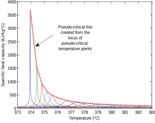
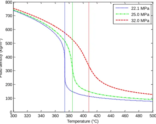
As shown in Figure 1.5, at supercritical pressures, no matter what the temperature is, there will be no gaseous phase. However, the fluid may transform to compressed liquid and finally to solid depending on how much the temperature is decreased. Critical temperature can be defined as no matter how much the fluid is compressed, there will be no liquid phase, but over critical temperature, supercritical fluid may transform into gaseous phase depending on the pressure. As clearly seen in the figure, in supercritical region, there is no co-existence of phase separation line since there are no phase changes above these thermodynamic conditions. This can be explained by the fact that when the pressure and temperature of the system on the blue boiling curve increase, the density of the fluid decreases and the density of the gas increases. At the critical point, these two densities become equal and the phase boundary between gas and liquid disappears [24]. Instead, we can define a new term in this region. This new curve shown in Figure 1.5 with dashed lines in the supercritical region is called the ‘pseudo-critical temperature line’. Pseudo-critical temperature line passes from pseudo-critical temperature points of corresponding pressure at supercritical region where the pseudo-critical temperature can be defined as the temperature that corresponds to the maximum value of the specific heat at a given pressure (i.e., at constant pressure). As shown in Figure 1.6, each supercritical pressure has its own pseudo-critical temperature. Moreover, as already mentioned, pseudo-critical temperature points altogether create a locus of pseudo-critical states as presented in Figure 1.6 (i.e., the specific heat as a function of temperature [25]). It is important to mention that while passing through this pseudo-critical line, even though there are no phase changes, other thermo-physical properties may change quite fast.

From Figure 1.7 to Figure 1.13, the change of thermo-physical properties as a function of temperature is shown for three different constant pressures. Since the change of thermo-physical properties at critical temperature is very important, the first pressure shown in these figures corresponds to the critical pressure of water (i.e, 22.1 MPa). Other pressure is the isobar of 25

MPa because most of the future nuclear reactor concepts will operate under this pressure [3, 5].

(40)

loop of École Polytechnique de Montreal, described in Chapter 2. In Figure 1.7 to Figure 1.13, the vertical solid lines show the position of pseudo-critical temperature point for each corresponding pressure.

At critical pressure, the specific heat theoretically goes to infinite (Figure 1.6) and the speed of sound decreases by 3.5 times (Figure 1.7) with increasing the temperature from 300°C to 374°C (i.e., critical temperature) and then starts increasing, but much slowly.

Figure 1.6 Specific heat capacity vs. fluid temperature for different constant pressures.

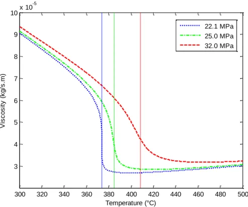
Within a temperature range of 300°C to 500°C the density decreases by a factor of 8 (Figure 1.8). The viscosity of the water decreases 3 times with increasing the temperature from 300°C to 374°C, then it stays almost constant (Figure 1.10). At higher pressures, these variations maintain almost the same ratios, but the slopes of the changes are much smaller.

373 374 375 376 377 378 379 380 381 382 383 0 500 1000 1500 2000 2500 3000 3500 4000 Temperature (°C) S p e c if ic h e a t c a p a c it y ( k J /k g °C ) Pseudo-critical line created from the

locus of pseudo-critical temperature points

(41)

Figure 1.7 Change of speed of sound as a function of temperature.

Figure 1.8 Change of density as a function of temperature. 300 320 340 360 380 400 420 440 460 480 500 200 300 400 500 600 700 800 900 1000 1100 Temperature (°C) S p e e d o f s o u n d ( m /s ) 22.1 MPa 25.0 MPa 32.0 MPa 300 320 340 360 380 400 420 440 460 480 500 0 100 200 300 400 500 600 700 800 Temperature (°C) F lu id d e n s it y ( k g /m 3) 22.1 MPa 25.0 MPa 32.0 MPa

(42)

Figure 1.9 Change of enthalpy as a function of temperature.

Figure 1.10 Change of viscosity as a function of temperature. 300 320 340 360 380 400 420 440 460 480 500 1000 1500 2000 2500 3000 3500 Temperature (°C) E n th a lp y ( k J /k g ) 22.1 MPa 25.0 MPa 32.0 MPa 300 320 340 360 380 400 420 440 460 480 500 3 4 5 6 7 8 9 10x 10 -5 Temperature (°C) V is c o s it y ( k g /s .m ) 22.1 MPa 25.0 MPa 32.0 MPa

(43)

Figure 1.11 Change of specific isobaric heat capacity as a function of temperature.

Figure 1.12 Change of specific isochoric heat capacity as a function of temperature. 300 320 340 360 380 400 420 440 460 480 500 0 10 20 30 40 50 60 70 80 90 100 Temperature (°C) S p e c if ic i s o b a ri c h e a t c a p a c it y ( k J /k g °C ) 22.1 MPa 25.0 MPa 32.0 MPa 300 320 340 360 380 400 420 440 460 480 500 2 2.5 3 3.5 4 4.5 5 Temperature (°C) S p e c if ic i s o c h o ri c h e a t c a p a c it y ( k J /k g °C ) 22.1 MPa 25.0 MPa 32.0 MPa

(44)

Figure 1.13 Specific heat ratio as a function of temperature.

For all thermo-physical properties, it is very important to mention that their variations close to pseudo-critical temperature are very drastic. However, for temperatures far away from the pseudo-critical value, variations in the thermo-physical properties become less significant. Also, as shown in from Figure 1.7 to Figure 1.13, when the pressure increases, the changes in the thermo-physical properties become smoother. For instance, if the pressure is increased over 50MPa, the peak of the property widens a lot and it makes almost impossible to determine the

exact location of pseudo-critical temperature. For some fluid properties, this peak becomes almost flat.

Since several safety calculations such as; depressurization rate, selection of safety valve, heat transfer are dependent on these thermo-physical parameters, it is very important to know the behaviour of the fluid at supercritical conditions. For example, the convection heat transfer coefficient will be highly influenced by the change of specific isobaric heat capacity. If pressure changes during a LOCA or even close to normal operation conditions, the integrity of the fuel may be affected due to a sudden increase of rod bundle surface temperatures. On the other hand,

300 320 340 360 380 400 420 440 460 480 500 0 2 4 6 8 10 12 14 16 18 20 Temperature (°C) S p e c if ic h e a t ra ti o 22.1 MPa 25.0 MPa 32.0 MPa

(45)

if the critical discharge flow rate at these pressures is unknown, it will be impossible to control the cooling conditions safely during an eventual LOCA.

The critical pressure and temperature of water are very aggressive in terms of magnitude, which makes it difficult to perform experiments with water compared to the ones with other fluids. As a result, carbon dioxide, helium and freon also are widely used at supercritical conditions [5, 26]; their critical conditions are given in Table 1.1 for comparison.

Actually, it is known that supercritical fluids exist in nature since the universe was formed but scientists discovered them in the late 1800s and they have been used in industrial applications only during the last 50-60 years mostly for food extraction, dry-cleaning, cleaning, cutting of high precision materials and coal fired boilers. Recently, the nuclear industry is also aimed to use supercritical fluids to increase the efficiency of the nuclear power reactors [27, 28].

Table 1.1 Critical parameters of fluids [5].

Fluid Pc (MPa) Tc (°C)

Carbon dioxide 7.38 30.98

Freon-134a 4.06 101.06

Helium 0.2275 -267.95

Water 22.06 373.95

As a result, the high interest of using supercritical fluids for industrial applications, in particular by the power industry in the last few years, increased the number of the research works in this area. Within this frame work, researchers have investigated the thermo-physical properties of fluid at supercritical conditions and the existence of a pseudo-critical line. Imre et al. [29] have studied the thermo-physical properties of water at supercritical conditions for pressures up to 50MPa. They determined a pseudo-critical line identified as the ‘Widom line’. Since for a given

pressure the maxima or minima for every thermo-physical property do not occur at the same temperature, for each fluid there is a collection of lines. Thus, there are several Widom lines instead of a single one. This set of lines delimits a zone called the Widom region. As a result, for any thermo-physical property, there is a Widom line that connects their maximum or minimum. However, there is only one pseudo-critical line [5] that corresponds to the locus of maxima of the

(46)

isobaric heat capacity at different constant pressures. Close to critical point the Widom lines approach each other and become almost identical to the pseudo-critical one. For the operation range of SCWR (about 25 MPa) the difference between these two definitions can be neglected. Researchers have also separated the supercritical region into two parts called liquid-like SCW and gas-like SCW [28], because a drastic change of thermo-physical properties occur, passing through one region to another. The liquid-like region is represented by triangle limited by the pseudo-critical temperature line and the constant critical temperature line at supercritical pressures. The gas-like region is delimited by a constant pressure line at supercritical temperatures and the pseudo-critical temperature line as shown in Figure 1.14.

Figure 1.14 Pressure-temperature diagram for water and liquid-like and gas-like supercritical regions.

Brazhkin et al. [30-32] have also separated the supercritical region into two zones, calling them solid-like and gas-like regions or rigid and non-rigid liquids. They used shear resistance parameter to define the crossover zone and introduced the gas-like region where the shear resistance disappears for any vibrational frequencies where significant changes in thermo-physical properties occur. They call this line as ‘Frenkel line’ in honor of Frenkel’s contributions

200 250 300 350 400 450 500 550 600 0 5 10 15 20 25 30 35 Temperature (°C) P re s s u re ( M P a ) Liquid Critical point Liquid like region Superheated steam Supercritical fluid Compressed fluid

Pseudo-critical temp. line Gas like

region

Saturation line