LIQUIDITY AND VOLATILITY IN THE AMERICAN CRUDE OIL FUTURES MARKET
Delphine LAUTIER & Fabrice RIVA
Delphine Lautier is Assistant Professor at the University Paris Dauphine. Postal Address: Cereg
University Paris Dauphine
Place du Maréchal de Lattre de Tassigny
75 775 Paris Cedex 16
Telephone number: 33 (1) 44 05 46 42 Fax : 33 (1) 44 05 40 23
Email: Delphine.Lautier@ dauphine.fr
Fabrice Riva is Assistant Professor at the University Paris-Dauphine. Postal Address: Cereg
University Paris Dauphine
Place du Maréchal de Lattre de Tassigny
75 775 Paris Cedex 16
Telephone number: 33 (1) 44 05 49 88 Fax : 33 (1) 44 05 40 23
LIQUIDITY AND VOLATILITY IN THE AMERICAN CRUDE OIL FUTURES MARKET
Delphine LAUTIER & Fabrice RIVA
CEREG
University Paris-Dauphine
First draft: 07/05/2004
ABSTRACT. This article focuses on the impact of derivative markets on the American crude oil market.
It first analyses the depth and liquidity of the market, and shows that there is a huge increase in activity from 1989 to 2003. Then the study focuses on prices volatility. The latter is separated into two components: an information component, that reflects a rational assessment of the information arrival, and an error component, that represents the noise introduced by the trading process. We show that a significant part of the volatility recorded during exchange trading hours is due to mispricing errors.
KEY WORDS: volatility – crude oil – noise trading – trading volumes – open interest – information
This article aims at answering the following questions: does the existence of derivatives markets have an undesirable influence on the behaviour of the underlying commodities? Do the commodity markets become nowadays more volatile, more speculative than before? These questions gained in importance during the last decade, as a result of the intensified presence of certain categories of investors such as hedge funds. The untimely and heavy interventions of these actors could indeed have an impact on the prices. Whereas this problem is relevant for all markets, it is especially important for commodity markets, because in this context, the real and financial spheres are intimately associated.
The theoretical framework of our study is the microstructure of financial markets. Through the study of the depth and liquidity of the market and the determinants of volatility, it aims at examining the informational content of commodity futures prices. This could be a first step in a work aiming to
appreciate the quality of the services produced by the futures markets, namely the redistribution of risk between different categories of operators which are more or less risk averse, and the promotion of informative signals – the futures prices. Our method consists in decomposing volatility into two components: the first one is called fundamental volatility and comes from the physical market; the second one is the volatility caused by trading. On a practical point of view, the interest of this work is twofold. Firstly, it should give a way to better appreciate the efficiency of hedging strategies. Secondly, it is important for regulatory purposes.
The problem of volatility is especially important for energy markets, as they become more and more integrated. As a result of tightened cross market linkages, a shock induced by the traders can spread not only to the physical market but also to other energy markets. Among the different energy markets, we focused on the American crude oil futures market because it is nowadays the most developed commodity market. Thus, information on futures prices, but also on transaction volumes and open interest, is abundant. The work is undertaken on a long period of time – 15 years, from January 1989 to December 2003 – in order to study how the market evolves, and to compare the more recent period – during which hedge funds are susceptible of intervening more intensely – to previous ones.
This article is organized as follows. Section 1 is devoted to the previous literature on the subject. Section 2 presents an overview of the evolution of the American crude oil futures market and on the way it comes to maturation through time. Section 3 is centred on the determinants of volatility.
SECTION 1. PREVIOUS LITERATURE
Literature on the impact of derivatives on commodity markets is relatively scarce. Among the available articles1, three different directions can be identified. The first one consists in directly investigating the influence of derivative markets. The second focuses on co-movements of commodity prices and spatial integration. The third examines the extent to which speculative trading could influence market prices and price informativeness.
Fleming and Ostdiek (1999) examine the effect of energy derivatives trading on the crude oil market between 1989 and 1997. They focus, first of all, on the introduction of new contracts on the market and their impact on volatility. They observe an abnormal volatility after the introduction of crude oil futures. However, subsequent introductions of crude oil options and derivatives on other energy commodities seem to have no effect. Then the authors examine the influence of derivatives trading on the depth and liquidity of the market. Their analysis reveals a strong inverse relationship between the open interest in crude oil futures and spot market volatility. Specifically, when open interest is greater, the volatility shock associated with a given unexpected increase in volume is much smaller. This finding indicates that the futures market provides depth and liquidity to the crude oil market.
The influence of derivatives on the commodity markets was also examined through the such-called ‘herding phenomenon’. In 1990, Pindick and Rotenberg propose to define herding by a situation where traders are alternatively bullish or bearish on all commodities for no plausible economic reasons. According to these authors, herding is a possible explanation for the excess co-movement that they observe on the prices of seven different commodities. Pindick and Rotenberg show first of all that the prices of raw commodities have a persistent tendency to move together. They try to explain this co-movement by macro-economic variables: the expected inflation, the growth in industrial production, the consumer price index, several exchange rates, interest rates, money supply, and the S&P common stock index. However, they find that the co-movement is well in excess of anything that could be explained by these common variables, and they conclude that herding could explain this excess. Booth and Cinner (2001) extend this work. They analyse the linkage among agricultural commodity futures prices on the Tokyo Grain Exchange, and they suggest two explanations of long-term co-movements among the prices of agricultural futures contracts: common economic fundamentals or herd behaviour by market participants. Contrary to Pindick and Rotenberg, their results support the common economic fundamentals assumption.
Another way to deal with the subject of derivatives and their impact on commodity prices is to focus on the spatial integration of commodity prices. Indeed, integration can be seen as a way to reinforce the impact of a derivative market on underlying markets, through the linkages between cash
markets. Spatial integration is most of the time examined through the methodology of co-integration and Granger causality tests.
Jumah, Karbuz and Rünstler (1999) study the spatial integration in the cocoa market, using prices extracted from London and New York markets. Interest rates are found to play a key role in establishing stationary long-run relationships. The authors also observe that futures prices Granger-cause spot prices, and that the reverse is not true. This is consistent with the view that futures prices adjust more quickly to new information compared to spot prices. Ewing and Harter (2000) study the co-movements of Alaska North Slope and UK Brent crude oil prices. Their results show that these oil markets share a long-run common trend, which suggests that the two markets are ‘unified’: there is price convergence in the markets. Kleit (2001) also examine the spatial integration of the crude oil markets. He studies seven types of crude oils. All of them are light crude oils, in order to reduce problems associated with quality differentials. His results show that oil markets are growing more unified. Milonas and Henker (2001) identify the variables that influence the relative price differentials of the Brent crude oil and the West Texas Intermediate. They show that the prices spreads are affected by convenience yields, which act as surrogates for demand/supply conditions and market price behaviour. Sanjuan and Gil (2001) study the spatial price relationship between European pork and lamb markets. The results indicate that markets for both commodities are integrated, not only in the long-run but in the short-run as well, although the price transmission process is more efficient in the pork meat industry.
All these works are important because spatial integration could exaggerate the possible negative influence of derivatives on the physical markets. However, they do not directly take into consideration the possible influence of derivatives.
The debate on the effects of derivatives trading is also closely related to the issue of the extent to which speculative trading could influence market prices and price informativeness. Several works have explored this field in the case of commodity markets. Foster (1995) shows that volume and volatility are contemporaneously correlated in the crude oil market. He suggests that both variables are influenced by the rate of information arrival. Moreover, he shows that the lagged volume explains prices variability, and concludes that the market is characterized by a certain degree of inefficiency. In
2000, Mossa and Silvapulle also present some evidence of a causal relationship between price and volume in the crude oil market. Using not only prices and volumes, but also open interest and prices spreads, Girma and Mougoué, in 2002, confirm the results obtained by Foster in the crude oil market. Ciner (2002) finds similar results on the Japanese commodity markets. Thus, all these work conclude to a relative inefficiency of commodity markets, which might be due to the impact of derivatives markets by an effect of mimetic contagion.
Among all these different works, our study belongs to the third approach, the one centred on price informativeness. Three reasons lead us to work in this direction.
The first is the lack of reliable time series for the spot prices. Indeed, in most commodity markets, the spot price is regarded as a non observable variable because physical markets are geographically dispersed, transactions are not standardized, the prices reporting mechanism does not enforce the operators to disclose their transactions prices, etc. In the case of the United States crude oil market, spot prices are also affected by other problems specific to this market. The trading volume for the West Texas Intermediate grade, namely the underlying commodity of the futures contract, is very low and the spot prices only provide information for local supply and demand. Moreover, there are sometimes problems due to an under-capacity of the pipeline system, which can create prices jumps. The latter are due to the delivery system, no to general market conditions. This phenomenon, reported by Horsnell and Mabro (1993), is known as the “Cushing Cushion”, because usually difficulties arise at Cushing Oklahoma, which is the delivery point of the futures contract. Thus, it seems difficult, in the case of the American crude oil market, to deal directly with the relationship between spot and futures markets. Consequently, we focused our attention on the available information, namely the information relative to futures prices.
Our second choice was to renounce to study the impact of the introduction of futures contracts. This kind of event is indeed not so frequent, and we were more interested, at least in the first step of the study, in the behavior of specific operators and in the way derivatives markets could be used than in the impact of the presence of new instruments.
Our third choice consists in using the methods and concepts of microstructure. The latter were not extensively used in the case of commodities, probably because the quite recent availability of high
frequency data on stock prices created a new field of researches and attracted a lot of attention. In commodity markets, the data are indeed not so abundant than they are elsewhere. However, there is still work to be done with the available information. Indeed, whereas settlement prices, open interest and trading volumes have already been exploited, little or no attention has been paid, nowadays, to the information given by prices curve – the relationship between futures prices having different maturities – or by opening and closing prices, or even intraday data, namely the highest and lowest prices recorded during the trading session. Yet, as we will see in the following study, they give precious indications on the volatility of futures markets and on the behaviour of operators.
SECTION 2. DATA AND DESCRIPTIVE STATISTICS
The first part of the study is devoted to the analysis of the market’s evolution from 1989 to 2003. Attention is focused, more particularly, on the liquidity and depth of the market. The latter are indeed two characteristics liable to attract speculators in the market, because it lowers the cost of their intervention in the market. Liquidity and depth are respectively approximated by trading volumes and open interest. These indicators give some precious indications on the relative importance of hedging and financial operations, and on the behaviours of the operators on the market.
In this section, we first of all present the data, then the evolution of trading volumes and open interest. Lastly, we present an analysis of the roll over strategies undertaken by the operators.
2.1. Data
The data used for the study are related to the light, sweet crude oil futures contract of the New York Mercantile Exchange (Nymex). All data have been operated such as the reconstituted time series always correspond to fixed monthly maturities. Indeed, the Nymex calendar was reconstructed in order to determine when a specific contract has, for example, a one- or a two-month maturity and to determine when the contract falls from the two-month to the one-month maturity. We collected first of all daily futures prices, corresponding to the opening and settlement prices, and to the highest and lowest prices recorded during the trading session. We also reconstituted monthly times series for the trading volume and open interest.
We extracted our data from Datastream, which leaded us to make certain choices. Indeed, for the trading volumes and open interests, when there was a zero at a specific date and maturity, it was impossible to know whether this zero corresponds effectively to an absence of transaction or open interest, or to an error. Moreover, when there was no information at a specific date and maturity, it was impossible to know whether this absence of information corresponds to a true missing value or to an absence of transaction or open interest. In order to render the data homogeneous, we decided to treat all zeros and missing values as missing values. This leads to a little overestimate of the trading volumes and open interests of the longer maturities, as activity is quite low for these delivery dates. However, the impact is negligible. Another consequence is that we only consider that there is information when there is no missing value. Thus, we can not take into account, as in Jones, Kaul and Lipson (1994) the fact that the absence of trading provides information.
Our sample period is 15 years long and ranges from January 1989 to December 2003. The choice of such a long period of time gives the possibility to examine the evolution of the market. As the latter came to fruition, some new futures contracts with longer maturity were introduced. Thus, the futures prices do not always have the same maturity in this database. For example, information relative to long-term contract (seven years maturity) is only available on the period 1997-2203.
2.2. Trading volumes
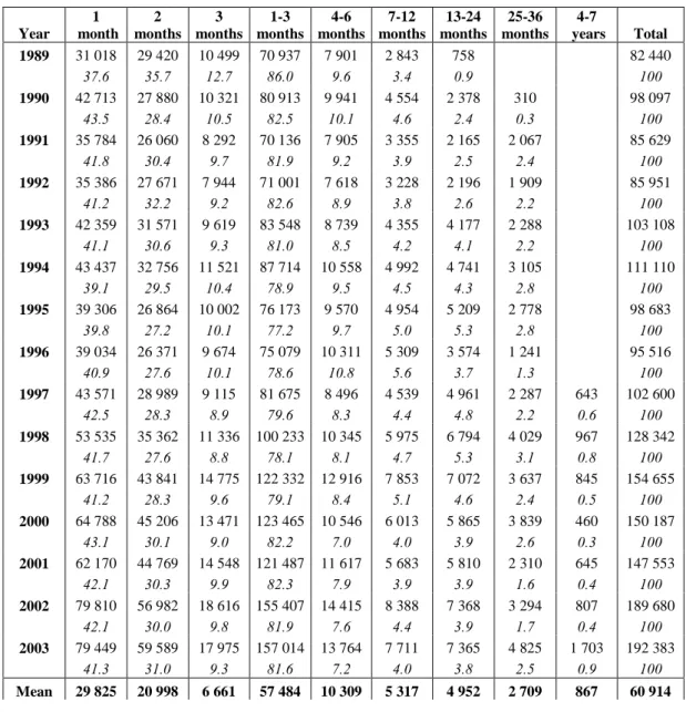
Trading volumes are a first simple indicator of the liquidity of a market. Table 1 summarizes descriptive statistics concerning this indicator on the sample period. It reproduces the average daily trading volumes, sorted by groups of maturities (1 to 3 months, 4 to 6 months, 7 to 12 months, 13 to 24 months, 25 to 36 months, and 4 to 7 years), year by year. As liquidity is usually concentrated on the shorter maturities in commodity markets, a special attention is paid to the first three months.
Table 1 indicates first a strong increase in the liquidity of the light, sweet crude oil futures contract during the period: trading volumes gain more than 133%, from a daily average of 82 440 futures contracts in 1989 to 192 383 contracts in 2003. However, as shown in Figure 1, the evolution is not totally regular: three sub-periods are indeed characterised by a decrease in the trading volumes.
The explanation lies in the outcome of specific events that affected the crude oil market: the 1st Gulf War in 1990-1991, the Metallgesellschaft crisis in 1994-1995 and the Enron crisis in 1999-2000.
The market strongly reacted to these events, and the reaction lies in a reduction in the trading volume. However, on the whole period, the market displays a huge increase in activity. This increase does not necessarily affect all the maturities in the same way. In order to verify this assumption, it is necessary to give evidence about the distribution of volumes among maturities, and their evolution through time.
Figure 1. Trading volumes, 1989-2003 (Number of futures contracts)
7 0 0 0 0 9 0 0 0 0 1 1 0 0 0 0 1 3 0 0 0 0 1 5 0 0 0 0 1 7 0 0 0 0 1 9 0 0 0 0 1 9 8 9 1 9 9 0 1 9 9 1 1 9 9 2 1 9 9 3 1 9 9 4 1 9 9 5 1 9 9 6 1 9 9 7 1 9 9 8 1 9 9 9 2 0 0 0 2 0 0 1 2 0 0 2 2 0 0 3
A striking feature of derivatives markets, as far as liquidity is concerned, is the concentration of trading activity on shorter maturities. This phenomenon is well known in derivatives markets, whatever the underlying asset is considered. The American crude oil futures market respects this rule. Indeed, as shown in Table 1, where the proportion of each maturity group in the cumulated trading volume is given in parentheses, the first three contracts account for 81.6% of the cumulated trading volume in 2003, and almost 97% of the trading volume is concentrated on maturities below 2 years. Considering the fact that there are delivery dates up to seven years, this figure could be interpreted as the sign of an extreme concentration on the shorter maturities. However, a comparison with the
currency market shows that the crude oil market is rather well balanced. Indeed, in the forward currency market, which is well-known for its liquidity and efficiency, maturities longer than one year only account for 1% of the trading volume2!
Focusing now on the nearest three contracts, it is possible to show that their share in the total trading volume is rather stable on the whole period. The first contract represents in average 41.4% of the total trading volume, the second contract 29.8%, and the third 9.8%. However, this stable structure reflects a relative increase in the liquidity of the shorter contracts because the number of traded maturities rises significantly in the crude oil market during the period: this number was multiplied by three, from 11 monthly maturities in 1989 to 33 in 2003.
Table 1. Descriptive statistics, trading volumes (*)
Year 1 month 2 months 3 months 1-3 months 4-6 months 7-12 months 13-24 months 25-36 months 4-7 years Total 1989 31 018 29 420 10 499 70 937 7 901 2 843 758 82 440 37.6 35.7 12.7 86.0 9.6 3.4 0.9 100 1990 42 713 27 880 10 321 80 913 9 941 4 554 2 378 310 98 097 43.5 28.4 10.5 82.5 10.1 4.6 2.4 0.3 100 1991 35 784 26 060 8 292 70 136 7 905 3 355 2 165 2 067 85 629 41.8 30.4 9.7 81.9 9.2 3.9 2.5 2.4 100 1992 35 386 27 671 7 944 71 001 7 618 3 228 2 196 1 909 85 951 41.2 32.2 9.2 82.6 8.9 3.8 2.6 2.2 100 1993 42 359 31 571 9 619 83 548 8 739 4 355 4 177 2 288 103 108 41.1 30.6 9.3 81.0 8.5 4.2 4.1 2.2 100 1994 43 437 32 756 11 521 87 714 10 558 4 992 4 741 3 105 111 110 39.1 29.5 10.4 78.9 9.5 4.5 4.3 2.8 100 1995 39 306 26 864 10 002 76 173 9 570 4 954 5 209 2 778 98 683 39.8 27.2 10.1 77.2 9.7 5.0 5.3 2.8 100 1996 39 034 26 371 9 674 75 079 10 311 5 309 3 574 1 241 95 516 40.9 27.6 10.1 78.6 10.8 5.6 3.7 1.3 100 1997 43 571 28 989 9 115 81 675 8 496 4 539 4 961 2 287 643 102 600 42.5 28.3 8.9 79.6 8.3 4.4 4.8 2.2 0.6 100 1998 53 535 35 362 11 336 100 233 10 345 5 975 6 794 4 029 967 128 342 41.7 27.6 8.8 78.1 8.1 4.7 5.3 3.1 0.8 100 1999 63 716 43 841 14 775 122 332 12 916 7 853 7 072 3 637 845 154 655 41.2 28.3 9.6 79.1 8.4 5.1 4.6 2.4 0.5 100 2000 64 788 45 206 13 471 123 465 10 546 6 013 5 865 3 839 460 150 187 43.1 30.1 9.0 82.2 7.0 4.0 3.9 2.6 0.3 100 2001 62 170 44 769 14 548 121 487 11 617 5 683 5 810 2 310 645 147 553 42.1 30.3 9.9 82.3 7.9 3.9 3.9 1.6 0.4 100 2002 79 810 56 982 18 616 155 407 14 415 8 388 7 368 3 294 807 189 680 42.1 30.0 9.8 81.9 7.6 4.4 3.9 1.7 0.4 100 2003 79 449 59 589 17 975 157 014 13 764 7 711 7 365 4 825 1 703 192 383 41.3 31.0 9.3 81.6 7.2 4.0 3.8 2.5 0.9 100 Mean 29 825 20 998 6 661 57 484 10 309 5 317 4 952 2 709 867 60 914
2 Source : BIS Quarterly Review, various issues.
Dtb(**) 41.3 29.8 9.8 80.9 8.7 4.4 3.7 2.0 0.3 100.0 Max 218 922 209 260 56 019 484 531 33 489 19 304 24181.0 6 695 47 216 218 922
∆∆∆∆(***) 156.1 102.5 71.2 110.0 78.7 192.4 281.8 182.9 143.3 133.4 Std-Err 23 008 22 428 7 079 17 505 2 538 1 266 779 520 720 2 287
(*) Percentage of each maturity in the cumulated trading volume is given in italic (**) Average distribution on the period, in percentage
(***) Changes recorded, in percentage, between 1989 and 2003
Thus, liquidity – measured by the trading volume – increases in the crude oil market during the period. It is strongly concentrated on the nearest contracts, and this concentration rises with time. Two reasons can be invoked to explain that phenomenon. Firstly, it could be due to an increase of the relative importance of speculators in the market. These operators usually have a very short trading horizon. Secondly, it could be explained by a change in the practices of the operators, leading them to take shorter positions and roll them over as the contract reaches maturity. This procedure could also be a result of the increasing liquidity on the nearest contracts and contribute, in return, to increase the liquidity. In the remaining of this study, we will try to discriminate between these two possible explanations.
2.3. Open interest
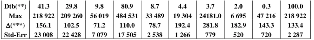
The open interest is another indicator of the liquidity of the market. Indeed, it can be regarded as a proxy of the depth of a market. Table 2 summarizes descriptive statistics concerning this indicator on the sample period. It reproduces the average daily open, sorted by groups of maturities, year by year. Once again, a special attention is paid to the first three months.
Table 2 shows that the open interest increases strongly during the period. It gains 140%, from a daily average of 233 382 futures contracts for the whole market in 1989 to 569 395 contracts – namely 570 millions of barrels – in 2003. As is the case for the trading volume, the rise in the open interest is not regular: it decreases sharply in 1994-1995 and in 1999-2000. However, as far as open interest is concerned, the first Gulf war (1990-1991) does not appear as a particular period. Thus, the two indicators do not always evolve in the same way – in 1990, open interest rises whereas trading volume decreases – and when crises have an impact on open interest, this impact seems to be stronger
on open interest. Moreover, open interest rises a bit more rapidly than the trading volume: +144% for the for the former, +133% for the latter. As speculators tend to initiate and compensate their position during the same trading day, this phenomenon indicates that the market tends to be more intensely used for hedging purposes.
The open interest is also concentrated on the shortest maturities, as shown in Table 2. However, concentration diminishes through time. Indeed, the first three contracts accounted for 64.1% of the cumulated open interest in 1989. This proportion decreases to 49.2% in 2003. Thus, if the introduction of new futures contracts having a longer maturity has no real impact on the distribution of trading volume through maturities, it influences the balance of open interest. The concentration on the shortest maturities diminishes. Consequently, in 2003, futures contracts having a maturity lower than one year account for 79% of the open interest, whereas in 1989, maturities below twelve months concentrate 97% of the open interest.
Table 2. Descriptive statistics, Open interest(*)
Year 1 month 2 months 3 months 1-3 months 4-6 months 7-12 months 13-24 months 25-36 months 4-7 years Total 1989 56476 59847 33251 149574 49079 27702 7027 233382 24,2 25,6 14,2 64,1 21,0 11,9 3,0 0,0 0,0 100 1990 59197 54584 33188 146969 52897 51735 23849 385 275834 21,5 19,8 12,0 53,3 19,2 18,8 8,6 0,1 0,0 100 1991 58701 52490 30939 142130 58733 49373 38792 36020 325048 18,1 16,1 9,5 43,7 18,1 15,2 11,9 11,1 0,0 100 1992 61691 61303 36083 159078 61228 51544 62671 69529 404049 15,3 15,2 8,9 39,4 15,2 12,8 15,5 17,2 0,0 100 1993 81655 73678 38974 194307 68489 64674 84392 95732 507594 16,1 14,5 7,7 38,3 13,5 12,7 16,6 18,9 0,0 100 1994 81292 76996 43227 201515 69778 66896 81714 109188 529090 15,4 14,6 8,2 38,1 13,2 12,6 15,4 20,6 0,0 100 1995 71685 66584 36771 175040 57393 58671 55968 24864 371936 19,3 17,9 9,9 47,1 15,4 15,8 15,0 6,7 0,0 100 1996 71933 65628 41630 179192 75245 79560 47083 9806 390886 18,4 16,8 10,7 45,8 19,2 20,4 12,0 2,5 0,0 100 1997 78894 68546 38624 186064 65954 68201 61285 42698 9028 433229 18,2 15,8 8,9 42,9 15,2 15,7 14,1 9,9 2,1 100 1998 90931 80886 46213 218030 75495 79481 62344 39021 19904 494275 18,4 16,4 9,3 44,1 15,3 16,1 12,6 7,9 4,0 100 1999 116033 103966 62289 282288 101167 103323 56853 48775 16832 609238 19,0 17,1 10,2 46,3 16,6 17,0 9,3 8,0 2,8 100 2000 100029 85937 42208 228174 72024 77675 60659 50264 17105 505901 19,8 17,0 8,3 45,1 14,2 15,4 12,0 9,9 3,4 100 2001 95760 84032 41316 221108 63575 72894 58050 37694 12901 466223 20,5 18,0 8,9 47,4 13,6 15,6 12,5 8,1 2,8 100
2002 117527 95593 44477 257596 75038 77222 52198 37634 14645 514332 22,9 18,6 8,6 50,1 14,6 15,0 10,1 7,3 2,8 100 2003 123779 104443 51774 279997 82150 87482 57280 39981 22506 569395 21,7 18,3 9,1 49,2 14,4 15,4 10,1 7,0 4,0 100 Mean 84372 75634 41398 201404 68550 67762 54011 45828 16132 456931 Dtb(**) 19,2 17,4 9,6 46,3 15,9 15,3 11,9 9,0 1,5 100 Max 206752 199982 125054 206752 93370 65580 41508 29190 13969 206752 ∆∆∆∆(***) 119,2 74,5 55,7 83,1 69,9 292,3 238,6 -21,1 158,6 144,0 Std. Err 37328 28855 13388 26524 9209 7594 5664 4745 2074 7344
(*) Percentage of each maturity in the total open interest is given in italic (**) Average distribution on the period, in percentage
(***) Changes recorded, in percentage, between 1989 and 2003
Lastly, the open interest is roughly three times higher than the trading volume in 2003 (2.9 in 1989). This figure signifies that the open interest changes every three trading days in the crude oil market, which is a quite important turn over. Indeed, the average daily open interest, in 2003, accounts for 280 days of Opec production! More precisely, the open interest, in 2003, represents 1.78 times the trading volume for the three first months (2.15 in 1989); 5.97 times the trading volume for the fourth to sixth months (6.31 in 1989); 11.6 times the trading volume for the 7th to 12th months (10.28 in 1989); 15.32 times the trading volume for the 13th to 24th months (9.25 in 1989); 10.87 times the trading volume for the 25th month to the 3rd year; 33.80 times the trading volume for the 4th to 7th years. This structure reflects the difference in the liquidity of the shorter and longer parts of the prices curve. The open interest is very stable on longer maturities.
Like the distribution of the trading volume, the distribution of the open interest is concentrated on the shorter maturities. However, open interest is more balanced than trading volume, and the longest maturities gain in importance with time. This evolution is contradictory with the assumption of a reduction in transactions horizon. It also confirms the fact that the market is less intensely used for speculation purposes. More precisely, the proportion of speculators on the longer maturities is probably low, and the long-term futures contracts are used as a way to manage residual risks associated with swaps.
The compared evolution of the trading volume and open interest leads to suppose that there is a link between the increasing liquidity – measured by trading volume – on the nearest contracts and roll over strategies. Indeed, the comparison between Tables 1 and 2 shows that on the sample period, trading volumes of the two nearest contracts rise more rapidly than open interest does (the figures are respectively +119.2% and +74.5% for open interest, and 156.1% and 102.5%, for trading volumes) whereas the total trading volume rises less rapidly than the total open interest. The rebalancing of open interest towards longer maturities indicates, however, that this phenomenon can not be due to a shortening of transactions horizon of the market as a whole. The second possible explanation is that the investors use roll-over strategies more intensely than before: they take positions on short-term contracts and, as these positions reach maturity, they move them from the one- to the two-month contract.
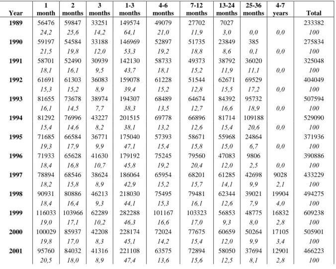
Figure 2 depicts the evolution of the open interest of the nearest two months during the end of the year 2003. There seems to be an inverse correlation between the two variables. Indeed, as the open interest of the first month decreases, the open interest of the second month increases. This phenomenon lasts until the expiration date of the nearby contract. Thus, a striking feature emerges by examining the joint evolution of the two first contracts: one contract seems to reflect the evolution of the other. One possible explanation for those antagonistic moves lies in the existence of roll-over.
Figure 2. Roll over, 11/21/2003-12/19/2003
0 50000 100000 150000 200000 250000 21/1 1/20 03 23/11/20 03 25/1 1/20 03 27/1 1/20 03 29/11 /200 3 01/1 2/2003 03/12/20 03 05/1 2/20 03 07/1 2/20 03 09/1 2/20 03 11/12/20 03 13/1 2/20 03 15/12/20 03 17/1 2/20 03 19/1 2/20 03 1st month 2nd month
In order to enlighten the existence of roll-over practices and their evolution through time, we performed several analyses. We first computed the correlation coefficient between the variations of the
two open interests. Then, we carried out a regression of the variation of the open interest of the second contract on the variation of the open interest of the first contract. A more precise investigation leads us to examine how the transfer between the two contracts evolves during the trading month. Lastly, in order to study the evolution of roll over practices on the sample period, we examined, year by year, how the open-interest on the one- and two-month contracts evolves as the nearby contract approaches its expiration date.
● Correlation between the changes in the open interests of the first- and second-months.
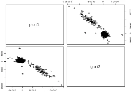
In order to give some evidence of roll-over practices, we first of all examined the relationship between the successive daily variations in the open interest of each contract. For each trading date and contract, we computed the variation in the open-interest recorded from one day to the subsequent one. Then we calculated the correlation between the variations attached to each contract. On the whole sample period, the correlation coefficient is –0.91 and is highly significantly different from zero. Moreover, as Figure 3 illustrates it, the correlation is particularly important when there are high variations in open interest (around 150 000 contracts) between two subsequent trading days. Thus, the two variables are all the more correlated than the trading volume is high.
Figure 3. Correlation between the changes in the open interest of the 1st and 2nd month contracts
p o i 1 - 1 5 0 0 0 0 - 5 0 0 0 0 0 5 0 0 0 0 -500 00 0 500 00 150 000 - 5 0 0 0 0 0 5 0 0 0 0 1 5 0 0 0 0 -1 500 00 -5 0 000 0 5 0 000 g o i 2
● Evidence of roll over practices
To further explore the relationship between the two contracts, we carried out a regression of the variation in the open interest of the second contract (∆OI2) on the variation of the open interest in the first contract (∆OI1):
t t
t OI
OI =α+β +ε
∆ 2 1
Rolling over the first nearby contract implies indeed that the open interest in the first month gets into the second month as the first months reaches maturity. Thus, the rise of the open interest of the second month contract should be explained by the decrease in the open interest of the first month. Table 3 reports the coefficients of the regression.
Table 3. Relationship between the open interest of the first and second contracts Estimate Stand. Error t-value Pr(>|t|)
α ß 300.64496 -0.58158 84.52183 0.00451 3.557 -128.941 0.00038 < 2e-16 Residual standard error: 4942 on 3438 degrees of freedom
Multiple R-Squared: 0.8286 Adjusted R-squared: 0.8286
F-statistic: 1.663e+04 on 1 and 3438 degrees of freedom p-value: < 2.2e-16
The coefficient ß associated with the decrease in open-interest on the one-month contract is less than one (in absolute value). This figure means that, on average, 58% of the position lost on the one-month contract gives rise to a similar increase in the position on the two-month contract. There are two possible destinations for the remaining 42%. Either it is rolled on maturities longer than 2 months or, more simply, this part of the position is compensated by the operators.
Another point of interest is the intercept value α. On average, the daily gain in the position on the two-month maturity that does not come from transfers of the one-month maturity corresponds to 300 futures contracts. Considering the fact that there are 23 trading days per month on average on the sample period, these 300 daily futures contracts represent an increase of 300 × 23 = 6,900 contracts in the open interest over a trading month. However, the open interest corresponds on average to 50,720
contracts at the beginning of the trading month and to 112,785 contracts at the end. Thus, the increase in the open interest that is not due to transfers from the one-month contracts only accounts for 11.12% of the increase!
● The evolution of the transfer from one contract to another through the trading month
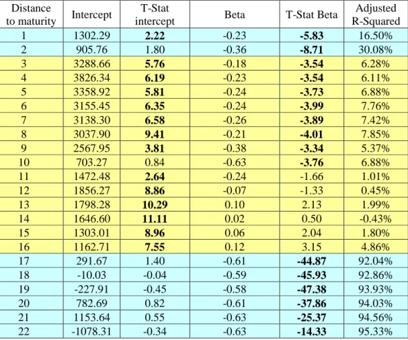
A more precise investigation consists in examining how the transfer between the two contracts evolves during the trading month. Table 4 reports the results of regressions that were run separately for each distance (or trading day) to the expiration of the one-month contract.
Table 4. Regressions for each distance to the maturity of the one-month contract. Distance
to maturity Intercept
T-Stat
intercept Beta T-Stat Beta
Adjusted R-Squared 1 1302.29 2.22 -0.23 -5.83 16.50% 2 905.76 1.80 -0.36 -8.71 30.08% 3 3288.66 5.76 -0.18 -3.54 6.28% 4 3826.34 6.19 -0.23 -3.54 6.11% 5 3358.92 5.81 -0.24 -3.73 6.88% 6 3155.45 6.35 -0.24 -3.99 7.76% 7 3138.30 6.58 -0.26 -3.89 7.42% 8 3037.90 9.41 -0.21 -4.01 7.85% 9 2567.95 3.81 -0.38 -3.34 5.37% 10 703.27 0.84 -0.63 -3.76 6.88% 11 1472.48 2.64 -0.24 -1.66 1.01% 12 1856.27 8.86 -0.07 -1.33 0.45% 13 1798.28 10.29 0.10 2.13 1.99% 14 1646.60 11.11 0.02 0.50 -0.43% 15 1303.01 8.96 0.06 2.04 1.80% 16 1162.71 7.55 0.12 3.15 4.86% 17 291.67 1.40 -0.61 -44.87 92.04% 18 -10.03 -0.04 -0.59 -45.93 92.86% 19 -227.91 -0.45 -0.58 -47.38 93.93% 20 782.69 0.82 -0.61 -37.86 94.03% 21 1153.64 0.55 -0.63 -25.37 94.56% 22 -1078.31 -0.34 -0.63 -14.33 95.33%
According to Table 4, it is possible to divide the trading month into three sub-periods. The first one ranges from day 22 (most of the time, the first trading date of the nearest contract) to day 17.
This period is characterised by the highest transfers from one contract to the other: the correlation coefficient is close to 1. During this period, roughly 60% of the one-month position is transferred to the two-month contract. One explanation for the persistence of the phenomenon over the five subsequent days lies in the fact that investors could span their interventions in order to mitigate the impact of their trades on prices. The second sub-period ranges from day 16 to day 3. This sub-period highly differs from the previous one as there is no significant correlation between the loss and gains on the two contracts, and the amount of the loss on the one-month contract that is transferred to the two-month contract is very low. The third sub-period covers the two last trading days. It is characterised by an increase in correlation. This might be due to investors who eventually decide to roll their position just before their contract expires.
Thus, this is mainly during the first part of the month that the roll over is carried out by investors. Indeed, they move their position from one month to the other one as soon as the contracts they hold fall into the one-month maturity. However, this result is obtained on the whole period. It does not take into account the increasing liquidity recorded between 1989 and 2003.
● Evolution of roll-over practices through time
In order to study the evolution of roll over practices during our sample period, we engaged ourselves in a year-by-year analysis on how the open-interest on the one- and two-month contracts evolves as the nearby contract tends towards its expiration date. Intuitively, as a result of the improved liquidity of the market, the roll over should be undertaken later in the trading month.
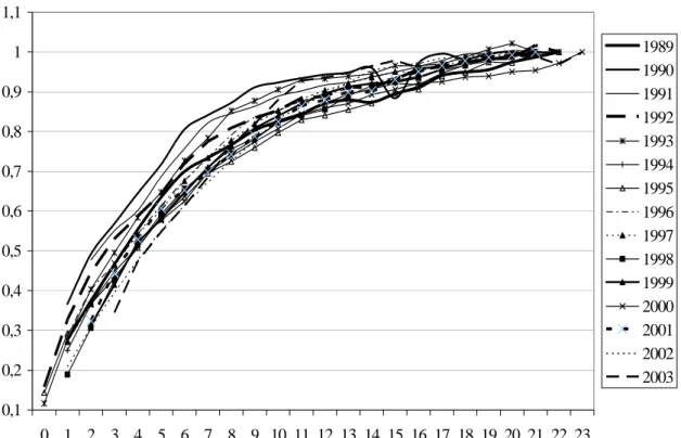
In this perspective, we constructed two time-series indicators representing the percentage of the open interest at a given date with respect to the open interest on a reference date. The reference date for the one-month contract is the first trading day for which the contract falls into the one-month maturity. The reference date for the two-month contract is defined as the expiration date of the one-month contract. By construction, the indicator values equal one at the reference dates. The evolution of our indicators are depicted by Figures 4 and 5.
A salient feature of Figure 4 is that the constitution of the open interest on the two-month contract gets more and more concentrated on the end of the trading months. Indeed, in 1989, 65% of
the final open-interest was already constituted at the beginning of the trading period (day 22), whereas this figure drops down to 40% in 2000 and the following years. Another striking aspect lies in the pace with which the open-interest evolves. During the first years of our sample period, the evolution is almost linear, that is, the open interest on the second- month contract regularly increases to reach its final level. In contrast, the most recent years are better characterised by an exponential trend. In 2002 for example, the open interest on the second month only increases by 10% over the first 13 trading days, whereas it increases by 50% during the last 10 trading days. This phenomenon highlights a significant change in the way investors trade future contracts. As the market evolves and becomes more and more liquid, they are able to take larger positions in relatively short time intervals.
Figure 4. Constitution of the open interest for the two-month futures contract
0,3 0,4 0,5 0,6 0,7 0,8 0,9 1 0 1 2 3 4 5 6 7 8 9 10 11 12 13 14 15 16 17 18 19 20 21 22 23
Distance to the expiration date of the one-month contract (in trading days)
Pe rce n tage of the f inal open-inter est 1989 1990 1991 1992 1993 1994 1995 1996 1997 1998 1999 2000 2001 2002 2003
Figure 5 exhibits similar exponential patterns, except that the evolution between the beginning and the end of the period is not as clear as before. However, it is possible to see that from 1989 to 2003, the de-constitution of the open interest of the one-month contract becomes a bit more rapid.
The evolution of the American crude oil futures market can be investigated through different kind of indicators. The steady introduction of new futures contract having a longer maturity is a first
sign of the good health of the market, as well as the improved liquidity, as measured by the trading volumes, and the increased depth of the market, approached by the open interest.
This improved liquidity has given rise to a change in the practices of the investors in the market. They tend to roll over their positions later in the trading month than before. Thus, the improved liquidity allows them to reduce the basis risk associated with the roll over strategies. Indeed, this risk – from the price change in closing out contracts –is less important at the end than at the beginning of the trading period.
The period is overall characterised by an increase in activity. Moreover, focusing on trading volumes and open interest shows that the relative importance of hedging or financial operations, and the behaviour of the operators on the market, have changed since 1989. The remaining question is the possible influence of these changes on volatility. This will be studied in the next part of the study.
Figure 5. De-constitution of the open interest of the one-month contract
0,1 0,2 0,3 0,4 0,5 0,6 0,7 0,8 0,9 1 1,1 0 1 2 3 4 5 6 7 8 9 10 11 12 13 14 15 16 17 18 19 20 21 22 23 1989 1990 1991 1992 1993 1994 1995 1996 1997 1998 1999 2000 2001 2002 2003
In this section, we first study the evolution of volatility, measured by the standard-error of prices changes, through time. This first overview will allow us to focus on some specific aspects of volatility and their evolution. More precisely, we will answer the following questions: does the trading process create a volatility in excess, which would not be observed in the absence of futures markets? Does this volatility change with the observation period?
3.1. The evolution of volatility during the observation period
Table 5 reproduces the volatility of the returns of settlement futures prices having a maturity between one and eight months, for each year of the observation period. The figures obtained a good illustration of the Samuelson effect3: the volatility of the returns strictly decreases with maturity.
Indeed, the most important feature of the commodity prices curve’s dynamic is probably the difference between the price behaviour of nearby and deferred contracts. The movements in the prices of the prompt contracts are large and erratic, while the prices of long-term contracts are relatively still. This results in a decreasing pattern of volatilities along the prices curve.
Table 5. Standard-error of the returns, settlement futures prices, 1989-2003
Year 1 month 2 months 3 months 4 months 5 months 6 months 7 months 8 months 1989 0,0216 0,0167 0,0153 0,0145 0,0144 0,0138 0,0135 0,0133 1990 0,0384 0,0286 0,0260 0,0254 0,0247 0,0242 0,0239 0,0236 1991 0,0312 0,0298 0,0253 0,0226 0,0209 0,0197 0,0186 0,0175 1992 0,0127 0,0122 0,0114 0,0108 0,0103 0,0099 0,0096 0,0093 1993 0,0154 0,0137 0,0127 0,0120 0,0114 0,0108 0,0105 0,0102 1994 0,0182 0,0162 0,0147 0,0137 0,0130 0,0125 0,0121 0,0117 1995 0,0128 0,0109 0,0096 0,0088 0,0082 0,0077 0,0074 0,0071 1996 0,0261 0,0192 0,0175 0,0159 0,0148 0,0141 0,0137 0,0134 1997 0,0056 0,0036 0,0035 0,0036 0,0034 0,0035 0,0036 0,0037 1998 0,0297 0,0251 0,0222 0,0204 0,0189 0,0177 0,0168 0,0160 1999 0,0223 0,0205 0,0191 0,0180 0,0172 0,0165 0,0160 0,0155 2000 0,0273 0,0240 0,0220 0,0206 0,0197 0,0189 0,0183 0,0179 2001 0,0275 0,0253 0,0233 0,0220 0,0210 0,0201 0,0192 0,0185 2002 0,0213 0,0195 0,0182 0,0171 0,0163 0,0156 0,0150 0,0145 2003 0,0243 0,0216 0,0196 0,0182 0,0169 0,0158 0,0149 0,0142 Average 0,0223 0,0189 0,0171 0,0160 0,0152 0,0146 0,0141 0,0137
3 Samuelson (1965).
The 1st Gulf War (1990 and 1991) excepted, the years of high volatility correspond, for each maturity, to 1998, 1999, 2000, 2001, 2002 and 2003. Yet, all these years are located at the end of our sample period. Thus, there seems to be an increase in the volatility of the crude oil futures prices, at least since 1998, as depicted by Figure 6.
There are several possible explanations for the increase in volatility: it could be the result of the deregulation in the energy markets, or it could be a consequence of improved informational efficiency (markets with greater trading volume exhibit sometimes greater volatility).
Figure 6. Standard-error of the returns, settlement futures prices, 1989-2003 (ex 1990-1991)
0,0000 0,0050 0,0100 0,0150 0,0200 0,0250 0,0300 1989 1992 1993 1994 1995 1996 1997 1998 1999 2000 2001 2002 2003 1 month 2 months 3 months 4 months 5 months 6 months 7 months 8 months
Considering this increase in volatility, it is interesting to see if the phenomenon affects homogeneously all the maturities. Whenever it appeared that the short-term prices become relatively more volatile than the long-term prices, the rise in the volatility could be attributed to a rise in the volatility of the cash market. The latter would propagate in the paper market, and would be progressively absorbed, as maturity progresses, via the Samuelson effect.
Table 6 illustrates, for each of the recent years, the impact of the volatility on the different maturities. It represents, indeed, for each year, the difference between the standard-error observed and the average calculated on the period (1990 and 1991 excepted). The results obtained show that the volatility of short-term prices rises more than the volatility of long-term prices in 1998, 2000, 2001,
and 2003. For these years, the gap with the average volatility is all the more high than the expiration date of the contract is close. This observation indicates that the increase of the volatility of crude oil futures prices could be explained by a rise in the fluctuations in the underlying market.
Table 6. Differences between the volatility observed and the average of the period
Year 1 month 2 months 3 months 4 months 5 months 6 months 7 months 8 months 1998 0,0094 0,0075 0,0061 0,0054 0,0046 0,0041 0,0037 0,0033 1999 0,0019 0,0029 0,0030 0,0030 0,0029 0,0029 0,0029 0,0028 2000 0,0069 0,0064 0,0059 0,0056 0,0054 0,0053 0,0052 0,0052 2001 0,0072 0,0077 0,0072 0,0070 0,0067 0,0065 0,0061 0,0058 2002 0,0009 0,0020 0,0021 0,0021 0,0020 0,0020 0,0019 0,0018 2003 0,0040 0,0040 0,0035 0,0031 0,0027 0,0022 0,0018 0,0014
3.2. The volatility caused by trading
One of the impacts of the presence of derivatives markets is that they can induce excess volatility, created by trading. In 1986, French and Roll proposed a method which allows to estimate the impact of trading on volatility. This part of our study is based on this method4.
The approach relies on the fact that prices are usually more volatile during trading hours than non trading hours. French and Roll consider three explanations for this phenomenon: i) volatility is caused by public information which is more likely to arrive during normal business hours; ii) volatility is caused by private information which affects prices when informed investors trade; iii) volatility is caused by pricing errors that occur during trading.
Following the authors, we first use different variance indicators to check whether the phenomenon of higher returns during trading hours is also observed in the case of the crude oil market. Indeed, this empirical observation has been pointed out by several authors in the case of equities, but it was left unexplored in the case of commodities. Then we try to identify and quantify, among the possible sources of volatility, the one which is caused by trading.
4 In the case of equities, information processing was further examined through the use of high frequency data. The latter are not publicly available in the case of the crude oil market. Yet we have data that are a bit more precise than those of French and Roll, because we can distinguish between opening and closing prices, which was not possible for the authors.
● Trading, overnight and weekend variances
In order to investigate whether there is noise trading in crude oil market prices, we first compare the volatility during the opening of the exchange, during the night, and during the weekend. We calculate different variance indicators, for each year and available maturity5 of our sample period.
The first indicator is called trading variance and corresponds to the variance of returns from open to close. The second indicator, the overnight variance, corresponds to the variance of returns from close to open. The third indicator is the week-end variance, namely the variance of returns from Friday close to Monday open.
The first two indicators correspond to periods where trading is conducted via different forms. Trading variances reproduces the way prices fluctuates in open outcry trading, and overnight variances represent the changes recorded when trading is conducted via an internet based trading platform provided by the Nymex, beginning at 3:15 pm on Mondays through Thursdays and concluding at 9:30 am the following day. On Sundays, the session begins at 7:00 pm. Thus, only week-end variances correspond to a period where there is no transaction and where the rate of information arrival is likely to be low6. Indeed, the crude oil market being a worldwide market, information can arrive at any hour
during the business day.
Figures 7 to 9 depict the evolution of these indicators over the whole sample period. Figure 7. Trading variances
5 The data relative on opening and closing prices are far less abundant than those relative to settlement prices. Consequently, we worked only on the first height months.
6 We do not have information concerning the proportion of the trading volume which is exchanged during the session of open
0 ,0 0 % 0 ,0 1 % 0 ,0 2 % 0 ,0 3 % 0 ,0 4 % 0 ,0 5 % 0 ,0 6 % 0 ,0 7 % 0 ,0 8 % 1 9 8 8 1 9 9 0 19 9 2 19 9 4 1 9 96 1 9 98 2 0 0 0 2 0 0 2 2 00 4 Y ear V ari ance 1 m on th 2 m on th 3 m on th 4 m on th 5 m on th 6 m on th 7 m on th 8 m on th
As was observed for the settlement prices, trading variances – the first Gulf War excepted – are higher in the second half of the period. Figure 7 also indicates that the one-month contract is always the most volatile, especially in the case of a crisis like the first Gulf War. Indeed, prices react as if the sole nearest month was absorbing the crisis. More generally, the trading variance of a given contract is inversely proportional to its maturity. Two combined effects can explain this phenomenon: the first is the Samuelson effect, which predicts that volatility is a decreasing function of maturity. The second is the trading volume, which is concentrated, as previously noted, on the nearest maturities. Indeed, a rise in the trading frequency increases the level of noise that is impounded into prices.
0,00 0,01 0,02 0,03 0,04 0,05 0,06 0,07 1988 1990 1992 1994 1996 1998 2000 2002 2004 Year Var iance in% 1 month 2 months 3 months 4 months 5 months 6 months 7 months 8 months
Variances recorded during the night appear to be lower than trading variances. This could be due to the fact that information arrival is actually less intensive during the night, because the market is concentrated in consumer areas, or to the fact that open outcry trading creates volatility in excess. Figure 8 also show that variances exhibit a rise in volatility at the end of the period, and special peaks around the first Gulf War. However, some differences with the previous results can be underlined. Firstly, the peaks of volatility are not the same for the two indicators. The peak recorded in 1998 for the trading variance disappears when overnight variance is considered. And during the first Gulf War, the peak of volatility does not correspond to 1990 but to 1991. Secondly, during periods of high volatility, the ordering of variances as a function of maturities can disappear, as is the case, for example, in 1991, in 1996 and in 2000.
Compared with the former indicators, weekend variances, depicted by Figure 9, are characterized by huge jumps during periods of crisis: in that case, variances can reach from 3 to 6 times their normal level. A probable consequence of the lack of volume during the weekend is that the hierarchy between contracts that was previously observed does not appear as clearly as before: more precisely, the one-month contract is not necessarily the most volatile, except when a crisis occurs. The Samuelson effect disappears, the ordering of contracts is almost unpredictable, especially during low volatility periods and the differences in volatility between the different maturities are quite low. Thus,
in the absence of volume, and probably also in the absence of arbitragers, the shocks transmission along the prices curve becomes impossible.
Figure 9. Week-end variances
0,00% 0,02% 0,04% 0,06% 0,08% 0,10% 0,12% 1988 1990 1992 1994 1996 1998 2000 2002 2004 Year Va ri an ce 1 month 2 month 3 month 4 month 5 month 6 month 7 month 8 month
Figure 7 to 9 show that both overnight and week-end variances are lower than trading variances. A simple indicator of the relative importance of these variances can be calculated: the ratio of overnight or week-end variances relative to trading variances. If hourly returns were constant across trading and non trading periods, the variance of weekend returns would be roughly 15 times the trading variance and the overnight variance would be roughly 5 times the trading variance7.
Table 7 reproduces the average variances ratios for each maturity during the whole sample period. The results are consistent with the evidence in earlier papers: the ratios are far less important than they should be, especially for the shorter maturities. They are lower for overnight variances than for week-end variances, which is normal. However, one could have expected a much higher difference between the two. This similarity leads to think, even if the information relative to volume during the night is not available, that overnight trading volume is quite low.
Table 7. Variance ratios, Overnight/Trading, and Week-end/Trading
1 month 2 months 3 months 4 months 5 months 6 months 7 months 8 months
7 The length of an outcry session is roughly 4 hours, namely (1/6) of a day. Thus, overnight trading is conducted during (5/6)
Overnight Average 0,538 0,566 0,451 0,437 0,568 0,617 0,618 0,612 Std Err 0,306 0,417 0,159 0,172 0,596 0,481 0,418 0,247 Week-end Average 0,649 0,719 0,623 0,661 0,710 0,763 0,740 0,832 Std Err 0,495 0,503 0,413 0,518 0,527 0,545 0,547 0,507
In order to give more insight on the relative importance of trading, overnight and week-end variances, these indicators must be normalized, so that the time span used for the computation of the variance is taken into account. For example, to compare trading and week-end variances, we took into account the fact that, from 1997 to November 2001, the trading session on the Nymex began at 9:45 am and ended at 3:10 pm, and that since 2001, it begins at 10:00 am and ends at 2:30 pm. Thus, there are 5.42 trading hours during the first sub-period, and 4.5 during the second. Likewise, during the first sub-period, the week-end period ranges from Friday 3:10 pm to Monday 9:45 am, that is 66.58 hours8?
During the second sub-period, it ranges from Friday 2:30 pm to Sunday 7:00 pm, due to the electronic system. If we consider, as a first approximation, that returns are independent, then the variance must be strictly proportional to the length of time used for its calculation. As a result, we can normalize our variances on an hourly basis.
The results concerning trading and non trading (weekend) variances are depicted on Figure 10. It shows that, on average on the whole period, the hourly trading variance is much higher than the week-end variance. More precisely, the former is 15.25 times the latter. Moreover, the hourly variances clearly decrease with maturity and consequently with activity. The same kind of results are obtained comparing the trading and overnight hourly variances. More precisely, on average on the period, for all maturities, the former is 10.14 times the latter.
Thus, in the American crude oil market, futures prices are much more volatile during the open outcry session. Two explanations can be invoked to explain this phenomenon. Firstly, it can be due to the fact that the rate of information arrival is higher during the opening of the exchange. The presence of a derivatives market, in that case, enables the prices to adjust more quickly to new information, and it introduces, as a consequence, more volatility. The second possible reason is that the process of
8 As no information is currently available about the opening and closing hours prior to 1997, we will consider that those hours are valid for the whole period.
trading introduces noise into returns. This noise can be due, for example, to operators who over-react to each other’s trade.
Figure 10. Trading and non trading (week-end) variances
0 0.00001 0.00002 0.00003 0.00004 0.00005 0.00006 0.00007 0.00008
1 month 2 month 3 month 4 month 5 month 6 month 7 month 8 month
H o u rly va ri an ce Non trading Trading
If the daily pricing error occurs during the trading period, it will not necessarily increase the trading-time variance. The increase will be observed only if some trading noise is not corrected during the trading day in which it occurs. Indeed, if all trading noise were corrected quickly, the noise would increase intra-day return variances, but it would not affect open to close returns.
At this point of the study, it is not possible to determine whether the information arrival or the noise trading dominates. The remaining of this study seeks to disentangle two components of volatility: an information component, that reflects a rational assessment of the information arriving during the day, and an error component.
In the next part of the study, we will examine the autocorrelation of daily returns, and we will compare daily return variances with variances for a long holding period.
More information on noise trading can be obtained by examining the autocorrelation of daily returns. Indeed, under the trading noise hypothesis, returns should be serially correlated: neither public nor private information will generate observable serial correlations.
Table 8 shows autocorrelations of futures prices returns for lags between one and twelve days. Autocorrelations are estimated during each year sub-period, using open to close returns. Table 8 also includes p-values associated with the autocorrelations. The main result is that futures prices returns are serially correlated. For all contracts, autocorrelations are significant9 at lag 4.
Table 8. Autocorrelations of daily trade returns for lags 1 to 12 One-month contract
Whole sample 1988-1993 1994-1999 2000-2003
Lag rho p-value rho p-value rho p-value rho p-value 1 0,0115 0,4835 -0,0638 0,0237 0,0707 0,0062 0,0226 0,4912 2 -0,0130 0,4285 -0,0255 0,3662 0,0167 0,5176 -0,0384 0,2410 3 0,0099 0,5487 0,0068 0,8095 -0,0216 0,4038 0,0549 0,0936 4 0,0768 0,0000 0,0673 0,0171 0,0693 0,0072 0,0971 0,0029 5 0,0053 0,7455 -0,0040 0,8873 0,0336 0,1933 -0,0216 0,5050 6 -0,0008 0,9619 0,0032 0,9110 -0,0103 0,6889 0,0065 0,8432 7 -0,0038 0,8191 -0,0062 0,8255 -0,0053 0,8370 0,0006 0,9861 8 0,0042 0,7999 0,0116 0,6815 0,0040 0,8770 -0,0054 0,8703 9 0,0178 0,2798 0,0591 0,0368 0,0295 0,2537 -0,0478 0,1430 10 0,0149 0,3663 0,0028 0,9213 0,0031 0,9052 0,0439 0,1774 11 0,0039 0,8127 0,0653 0,0210 -0,0290 0,2610 -0,0270 0,4098 12 0,0146 0,3763 0,0667 0,0185 -0,0077 0,7667 -0,0192 0,5581 # rho<0 3 4 5 6 Two-month contract Whole sample 1988-1993 1994-1999 2000-2003
Lag rho p-value rho p-value rho p-value rho p-value 1 0,0044 0,7898 -0,0666 0,0192 0,0502 0,0523 0,0172 0,5992 2 0,0028 0,8654 0,0168 0,5558 0,0312 0,2278 -0,0430 0,1895 3 0,0229 0,1658 0,0348 0,2219 -0,0099 0,7026 0,0496 0,1300 4 0,0742 0,0000 0,0653 0,0218 0,0698 0,0069 0,0871 0,0076 5 0,0187 0,2576 0,0322 0,2580 0,0345 0,1816 -0,0122 0,7066 6 0,0090 0,5844 0,0547 0,0547 -0,0189 0,4643 -0,0012 0,9707 7 -0,0050 0,7638 -0,0036 0,9006 -0,0032 0,9027 -0,0085 0,7949 8 0,0067 0,6872 0,0207 0,4686 0,0026 0,9210 -0,0016 0,9609 9 -0,0020 0,9058 0,0105 0,7128 0,0352 0,1730 -0,0565 0,0834 10 0,0224 0,1742 0,0274 0,3378 0,0119 0,6450 0,0298 0,3606 11 0,0045 0,7876 0,0266 0,3522 -0,0001 0,9974 -0,0111 0,7353 12 0,0262 0,1136 0,0899 0,0016 0,0007 0,9788 -0,0040 0,9037 # rho<0 2 2 4 8
9 It is quite surprising to note that the behaviour of the 8 futures contracts does not differ in terms of autocorrelations. One
could have expected that autocorrelations would change with liquidity and consequently with maturity. However, this is obviously not the case, even if the first month contract displays a number of significant autocorrelation that is a bit more important.
At lag 4, autocorrelations are always positive. Such positive autocorrelations support the trading noise hypothesis. Indeed, they could be due to over-reaction of traders to new information, this over-reaction persisting for more than one day. Consequently, the pricing error at day t+1 should be positively correlated to both information component at day t, and pricing error at t. Another possible explanation is that the market does not incorporate all information as soon as it is released. In that case, pricing error at day t should be negatively correlated with information at date t and pricing error at t+1 should be positively correlated with information at t. This positive autocorrelation between information at day t and pricing error at t+1 could generate positively autocorrelated returns.
Table 8 (continued) Three-month contract
Whole sample 1988-1993 1994-1999 2000-2003
Lag rho p-value rho p-value rho p-value rho p-value 1 0,0080 0,6300 -0,0180 0,5264 0,0421 0,1033 -0,0015 0,9629 2 0,0012 0,9444 0,0252 0,3736 0,0176 0,4961 -0,0452 0,1696 3 0,0294 0,0755 0,0366 0,1976 -0,0020 0,9377 0,0570 0,0831 4 0,0759 0,0000 0,0766 0,0069 0,0609 0,0185 0,0917 0,0052 5 0,0202 0,2214 0,0244 0,3916 0,0366 0,1567 -0,0034 0,9175 6 0,0090 0,5858 0,0209 0,4630 -0,0117 0,6500 0,0183 0,5786 7 0,0006 0,9701 -0,0058 0,8383 0,0103 0,6902 -0,0035 0,9149 8 -0,0043 0,7930 -0,0246 0,3869 0,0066 0,7972 0,0058 0,8610 9 0,0143 0,3865 0,0725 0,0107 0,0429 0,0974 -0,0844 0,0099 10 0,0172 0,2989 0,0019 0,9471 0,0165 0,5243 0,0345 0,2914 11 0,0118 0,4759 0,0395 0,1650 -0,0051 0,8448 -0,0014 0,9665 12 0,0186 0,2613 0,0715 0,0120 -0,0132 0,6090 -0,0060 0,8557 # rho<0 1 3 4 7 Four-month contract Whole sample 1988-1993 1994-1999 2000-2003
Lag rho p-value rho p-value rho p-value rho p-value 1 -0,0073 0,6568 -0,0457 0,1071 0,0285 0,2702 -0,0059 0,8583 2 0,0181 0,2719 0,0595 0,0361 0,0155 0,5497 -0,0231 0,4818 3 0,0212 0,1986 0,0264 0,3527 -0,0040 0,8761 0,0428 0,1932 4 0,0909 0,0000 0,0898 0,0015 0,0856 0,0009 0,0973 0,0030 5 0,0307 0,0626 0,0389 0,1703 0,0340 0,1877 0,0180 0,5807 6 0,0064 0,6965 0,0207 0,4671 -0,0248 0,3382 0,0244 0,4585 7 0,0111 0,5027 0,0089 0,7549 0,0101 0,6963 0,0138 0,6738 8 0,0012 0,9437 0,0000 0,9993 0,0002 0,9940 0,0030 0,9269 9 0,0031 0,8497 0,0277 0,3300 0,0341 0,1870 -0,0567 0,0833 10 0,0237 0,1502 -0,0204 0,4744 0,0266 0,3042 0,0660 0,0430 11 0,0263 0,1112 0,0521 0,0673 0,0180 0,4861 0,0075 0,8199 12 0,0254 0,1243 0,0737 0,0096 -0,0121 0,6394 0,0147 0,6549 # rho<0 1 2 3 3
Our last result is that negative autocorrelations tend to increase on the sample period, and they become dominant for certain maturities (2, 3, 6 and 7 months), at the end of the sample period.
Negative autocorrelations are also consistent with the trading noise hypothesis but the explanation of this phenomenon differs from the explanation of positive autocorrelations. Under the trading noise hypothesis, returns should be serially correlated, because pricing errors should be corrected in the long run. These corrections would generate negative autocorrelations.
Table 8 (continued) Five-month contract
Whole sample 1988-1993 1994-1999 2000-2003
Lag rho p-value rho p-value rho p-value rho p-value 1 -0,0291 0,0793 -0,0912 0,0013 0,0200 0,4407 -0,0172 0,6032 2 0,0109 0,5122 0,0250 0,3792 0,0297 0,2533 -0,0243 0,4636 3 0,0388 0,0195 0,0469 0,0997 0,0114 0,6618 0,0598 0,0709 4 0,0822 0,0000 0,0731 0,0102 0,0755 0,0036 0,0983 0,0029 5 0,0215 0,1948 0,0424 0,1372 0,0355 0,1715 -0,0153 0,6416 6 0,0211 0,2028 0,0473 0,0970 -0,0223 0,3910 0,0403 0,2247 7 0,0259 0,1184 0,0299 0,2949 0,0182 0,4825 0,0297 0,3712 8 0,0186 0,2618 0,0467 0,1019 -0,0028 0,9155 0,0121 0,7152 9 0,0068 0,6817 0,0228 0,4238 0,0426 0,1007 -0,0490 0,1377 10 0,0197 0,2359 0,0000 0,9993 0,0280 0,2812 0,0302 0,3596 11 0,0165 0,3201 0,0479 0,0936 0,0160 0,5387 -0,0161 0,6273 12 0,0199 0,2315 0,0599 0,0360 -0,0094 0,7170 0,0101 0,7605 # rho<0 1 1 3 5 Six-month contract Whole sample 1988-1993 1994-1999 2000-2003
Lag rho p-value rho p-value rho p-value rho p-value 1 -0,0040 0,8108 -0,0476 0,0973 0,0377 0,1519 0,0005 0,9890 2 -0,0008 0,9607 -0,0009 0,9764 0,0401 0,1280 -0,0478 0,1618 3 0,0426 0,0117 0,0452 0,1164 0,0253 0,3371 0,0572 0,0944 4 0,0777 0,0000 0,0817 0,0045 0,0764 0,0037 0,0722 0,0346 5 0,0208 0,2183 0,0429 0,1364 0,0326 0,2167 -0,0209 0,5387 6 0,0151 0,3728 0,0351 0,2232 -0,0182 0,4891 0,0263 0,4429 7 0,0228 0,1775 0,0342 0,2359 0,0378 0,1515 -0,0110 0,7471 8 0,0160 0,3443 0,0353 0,2213 0,0093 0,7242 -0,0013 0,9697 9 0,0031 0,8552 0,0245 0,3970 0,0419 0,1121 -0,0669 0,0499 10 0,0216 0,2018 0,0231 0,4246 0,0428 0,1045 -0,0055 0,8708 11 0,0063 0,7105 0,0209 0,4703 0,0160 0,5447 -0,0242 0,4800 12 0,0105 0,5336 0,0360 0,2132 -0,0065 0,8040 -0,0034 0,9216 # rho<0 2 2 2 8
To conclude on the subject of autocorrelations, our results are not especially satisfying. Daily returns appear to be serially correlated but, most of the time, the correlation coefficient are not significant. Moreover, there is no convincing explanation of the peak in autocorrelation at lag 4. Maybe an interesting study on autocorrelation could be done between open to close and close to open returns, because a significant part of the pricing error could be corrected during the night.
Another way to disentangle trading variance with information variance is to compare the variances computed on daily returns (which reflect information and pricing errors) with variances for a long holding period (which reflects information). This constitutes the next part of the study.
Table 8 (continued) Seven-month contract
Whole sample 1988-1993 1994-1999 2000-2003
Lag rho p-value rho p-value rho p-value rho p-value 1 0,0077 0,6584 -0,0243 0,3993 0,0479 0,0774 0,0003 0,9928 2 0,0289 0,0979 0,0236 0,4142 0,0588 0,0307 -0,0059 0,8734 3 0,0489 0,0052 0,0468 0,1057 0,0301 0,2692 0,0741 0,0476 4 0,0876 0,0000 0,0954 0,0009 0,0806 0,0031 0,0795 0,0326 5 0,0165 0,3443 0,0341 0,2384 0,0367 0,1777 -0,0406 0,2710 6 0,0078 0,6574 0,0421 0,1454 -0,0084 0,7585 -0,0288 0,4396 7 0,0138 0,4325 0,0444 0,1257 0,0104 0,7017 -0,0348 0,3514 8 0,0123 0,4825 0,0393 0,1745 -0,0061 0,8233 -0,0081 0,8272 9 0,0032 0,8563 0,0143 0,6214 0,0365 0,1805 -0,0591 0,1113 10 0,0348 0,0468 0,0283 0,3288 0,0508 0,0621 0,0212 0,5682 11 0,0057 0,7434 0,0056 0,8482 0,0369 0,1753 -0,0376 0,3134 12 0,0245 0,1622 0,0298 0,3045 0,0237 0,3849 0,0141 0,7047 # rho<0 0 1 2 7 Eight-month contract Whole sample 1988-1993 1994-1999 2000-2003
Lag rho p-value rho p-value rho p-value rho p-value 1 0,0095 0,6177 -0,0379 0,2083 0,0416 0,1673 0,0439 0,3036 2 0,0236 0,2160 0,0256 0,3950 0,0238 0,4322 0,0114 0,7890 3 0,0339 0,0763 0,0314 0,2993 0,0555 0,0660 0,0029 0,9456 4 0,0806 0,0000 0,1167 0,0001 0,0769 0,0109 0,0144 0,7389 5 0,0240 0,2106 0,0347 0,2518 0,0652 0,0312 -0,0618 0,1505 6 0,0172 0,3708 0,0003 0,9911 0,0119 0,6955 0,0475 0,2714 7 0,0214 0,2658 0,0653 0,0311 0,0109 0,7184 -0,0519 0,2304 8 0,0341 0,0766 0,0309 0,3075 0,0686 0,0241 -0,0123 0,7789 9 0,0154 0,4230 0,0067 0,8255 0,0434 0,1512 -0,0141 0,7431 10 0,0107 0,5774 0,0141 0,6418 0,0122 0,6898 -0,0046 0,9139 11 -0,0023 0,9051 0,0278 0,3598 0,0255 0,4028 -0,1008 0,0203 12 0,0081 0,6732 0,0226 0,4562 -0,0186 0,5403 0,0073 0,8672 # rho<0 1 1 1 6
● Comparison of daily return variances with variances for a long holding period.
This comparison of daily variances with variances for a longer holding period relies on the assumption that the importance of pricing errors diminishes as the holding period increases. Indeed, if daily returns were totally independent, the variance for a long holding period would equal the cumulated daily variances within this period. On the other hand, if daily returns are temporarily affected by trading noise, the longer period variance will be smaller than the cumulated daily