DÉPARTEMENT DE GÉOMATIQUE APPLIQUÉE Faculté des lettres et sciences humaines
Université de Sherbrooke
Amélioration des données altimétriques dans la région du Grand Lac des Esclaves à partir d’images Radarsat-2
Jean-Samuel Proulx-Bourque
Mémoire présenté pour l’obtention du grade de Maître ès sciences (M. Sc.) Cheminement recherche en télédétection
Février 2016
i
Directeur de recherche : Professeure Ramata Magagi Membre du jury interne: Professeur Alain Royer Membre du jury externe: Docteur Alexandre Beaulieu
ii
Résumé
En raison de sa grande étendue, le Nord canadien présente plusieurs défis logistiques pour une exploitation rentable de ses ressources minérales. La TéléCartographie Prédictive (TCP) vise à faciliter la localisation de gisements en produisant des cartes du potentiel géologique. Des données altimétriques sont nécessaires pour générer ces cartes. Or, celles actuellement disponibles au nord du 60e parallèle ne sont pas optimales principalement parce qu’elles sont dérivés de courbes à équidistance variable et avec une valeur au mètre. Parallèlement, il est essentiel de connaître l'exactitude verticale des données altimétriques pour être en mesure de les utiliser adéquatement, en considérant les contraintes liées à son exactitude. Le projet présenté vise à aborder ces deux problématiques afin d'améliorer la qualité des données altimétriques et contribuer à raffiner la cartographie prédictive réalisée par TCP dans le Nord canadien, pour une zone d’étude située au Territoire du Nord-Ouest. Le premier objectif était de produire des points de contrôles permettant une évaluation précise de l'exactitude verticale des données altimétriques. Le second objectif était de produire un modèle altimétrique amélioré pour la zone d'étude. Le mémoire présente d'abord une méthode de filtrage pour des données Global Land and Surface Altimetry Data (GLA14) de la mission ICESat (Ice, Cloud and land Elevation SATellite). Le filtrage est basé sur l'application d'une série d'indicateurs calculés à partir d’informations disponibles dans les données GLA14 et des conditions du terrain. Ces indicateurs permettent d'éliminer les points d'élévation potentiellement contaminés. Les points sont donc filtrés en fonction de la qualité de l’attitude calculée, de la saturation du signal, du bruit d'équipement, des conditions atmosphériques, de la pente et du nombre d'échos. Ensuite, le document décrit une méthode de production de Modèles Numériques de Surfaces (MNS) améliorés, par stéréoradargrammétrie (SRG) avec Radarsat-2 (RS-2). La première partie de la méthodologie adoptée consiste à faire la stéréorestitution des MNS à partir de paires d'images RS-2, sans point de contrôle. L'exactitude des MNS préliminaires ainsi produits est calculée à partir des points de contrôles issus du filtrage des données GLA14 et analysée en fonction des combinaisons d’angles d'incidences utilisées pour la stéréorestitution. Ensuite, des sélections de MNS préliminaires sont assemblées afin de produire 5 MNS couvrant chacun la zone d'étude en totalité. Ces MNS sont analysés afin d'identifier la sélection optimale pour la zone d'intérêt. Les indicateurs sélectionnés pour la méthode de filtrage ont pu être validés comme performant et complémentaires, à l’exception de l’indicateur basé sur le ratio signal/bruit puisqu’il était redondant avec l’indicateur basé sur le gain. Autrement, chaque indicateur a permis de filtrer des points de manière exclusive. La méthode de filtrage a permis de réduire de 19% l'erreur quadratique moyenne sur l'élévation, lorsque que comparée aux Données d'Élévation Numérique du Canada (DNEC). Malgré un taux de rejet de 69% suite au filtrage, la densité initiale des données GLA14 a permis de conserver une distribution spatiale homogène. À partir des 136 MNS préliminaires analysés, aucune combinaison d’angles d’incidences des images RS-2 acquises n’a pu être identifiée comme étant idéale pour la SRG, en raison de la grande variabilité des exactitudes verticales. Par contre, l'analyse a indiqué que les images devraient idéalement être acquises à des températures en dessous de 0°C, pour minimiser les disparités radiométriques entre les scènes. Les résultats ont aussi confirmé que la pente est le principal facteur d’influence sur l’exactitude de MNS produits par SRG. La meilleure exactitude verticale, soit 4 m, a été atteinte par l’assemblage de
iii
configurations de même direction de visées. Par contre, les configurations de visées opposées, en plus de produire une exactitude du même ordre (5 m), ont permis de réduire le nombre d’images utilisées de 30%, par rapport au nombre d'images acquises initialement. Par conséquent, l'utilisation d'images de visées opposées pourrait permettre d’augmenter l’efficacité de réalisation de projets de SRG en diminuant la période d’acquisition. Les données altimétriques produites pourraient à leur tour contribuer à améliorer les résultats de la TCP, et augmenter la performance de l’industrie minière canadienne et finalement, améliorer la qualité de vie des citoyens du Nord du Canada.
iv
Abstract
Due to its vast extent, Northern Canada faces several logistical challenges for a profitable exploitation of its mineral resources. Remote Predictive Mapping (RPM) aims to help in targeting mineral deposits through the production of geological potential maps. Elevation data is necessary for the generation of these maps. However, the currently available elevation data north of the 60th parallel are not optimal primarily because it has been derived from contours with values at a metric precision. Additionally, exact knowledge of the vertical accuracy of elevation data is essential to insure a suitable use, within its accuracy constraints. This project aimed to improve the quality of elevation data and to contribute to the refinement of RPM products for a study site located in the Northwest Territories. The first objective was to generate control points to evaluate vertical accuracy with precision. The second objective was to generate an improved elevation model for the study site. First, a filtering method for Global Land and Surface Altimetry Data (GLA14) from the ICESat (Ice, Cloud and land Elevation SATellite) mission is presented. This filtering is based on indicators, derived from information available in GLA14 data and terrain conditions, which are then applied successively to remove potentially contaminated elevation points. The points are filtered based on the attitude calculation, signal saturation, equipment noise, atmospheric conditions, slope and number of peaks. Next, a method to generate an improved Digital Surface Models (DSM) using StereoRadarGrammetry (SRG) with Radarsat-2 (RS-2) images is described. In the first part of the adopted methodology, DSM are stereorestituted from RS-2 image pairs, without control point. Then, the vertical accuracy of the DSM is calculated using the control points resulting from the filtering of GLA14 data, and analysed according to the incidence angles combination used for the stereorestitution. Next, selections from the preliminary DSM are assembled to generate 5 DSM, each covering entirely the study site. Finally, the DSM are analysed to identify the optimal selection for the area of interest. The selected indicators were found to be efficient and complementary, except for the indicator based on the noise/signal ratio. Otherwise, all indicators allowed to filter out points exclusively. A 19% reduction of the elevation mean square error was achieved with the filtering method, when compared to Canadian Digital Elevation Data (CDED). The initial density of the GLA14 allowed maintaining a spatially homogeneous distribution of the post-filtering elevation points despite a 69% rejection rate. From the analysis of the 136 preliminary DSM, no specific combination of the acquired RS-2 images incidence angles stood out as being ideal with SRG due to high variability in vertical accuracy. Nonetheless, the analysis showed that images should be ideally acquired at sub-zero temperatures to minimize radiometric discrepancies between scenes. Results also showed that the slope is the main factor influencing the accuracy of DSM generated with SRG. The best vertical accuracy (4 m) was achieved with same-side view configurations. Opposite-side view configurations, despite achieving a vertical accuracy of 5 m, allowed a 30% reduction in the amount of images initially acquired. Therefore, the use of opposite-side view configurations could help to improve the efficiency of SRG projects by reducing considerably the acquisition period. Elevation data generated using the proposed method could help to improve results from RPM and increase the efficiency of the mining industry in Northern Canada and finally contribute to the betterment of the lives of Northern Canada’s citizens.
v
Table des matières
RÉSUMÉ ... II ABSTRACT ... IV TABLE DES MATIÈRES ... V LISTE DES FIGURES ... VII LISTE DES TABLEAUX ... VIII ABRÉVIATION ... IX REMERCIEMENTS ... X
CHAPITRE 1 ... 1
1. INTRODUCTION...1
1.1. Problématique ...1
1.2. État des connaissances ...3
1.3. Objectifs ...6 1.4. Structure du document ...6 CHAPITRE 2 ... 7 2. MATÉRIEL ET MÉTHODE ...7 2.1. Site d’étude ...7 2.2. Données ...8 2.3. Méthodologie générale...11 CHAPITRE 3 ... 12
3. FILTRAGE DES DONNÉES GLA14 POUR DÉTERMINER L’EXACTITUDE VERTICALE DE DONNÉES D’ÉLÉVATION ...12
« FILTERING GLOBAL LAND AND SURFACE ALTIMETRY DATA (GLA14) FOR ELEVATION ACCURACY DETERMINATION » ...12
3.1. Présentation de l’article 1 ...12
3.2. Article 1 ...13
Abstract ...13
Introduction ...13
Study Site and Data ...14
Sources of Inaccuracy in GLA14 data ...16
Methodology ...18
Results and Discussion ...21
Conclusion ...27
Acknowledgments ...28
References ...29
CHAPITRE 4 ... 31
4. GÉNÉRATION DE MODÈLES NUMÉRIQUES DE SURFACE AU NORD DU CANADA PAR STÉRÉORADARGRAMMÉTRIE AVEC RADARSAT-2 ...31
«GENERATION OF DIGITAL SURFACE MODELS IN NORTHERN CANADA FROM STEREORADARGRAMMETRY WITH RADARSAT-2» ...31
4.1. Présentation de l’article 2 ...31 4.2. Article 2 ... Error! Bookmark not defined.
vi
Abstract. ...34
Introduction ...34
Background on Stereoradargrammetry ...36
Study Site and Data ...38
Method ...41
Results and Discussion ...45
Conclusion ...53 Acknowledgments ...55 References ...55 CHAPITRE 5 ... 58 5. CONCLUSION ...58 RÉFÉRENCES ...61
vii
Liste des figures
Figure 2-1: Localisation de la zone d'étude. ...7 Figure 2-2: Zone d'étude : Hydrographie et élévation. ...8 Figure 2-3: Organigramme simplifié du développement de données altimétriques améliorées ....11 Figure 3-1: The location of the AOI, marked by the dark area ...17 Figure 3-2: Outliers illustrated with respect to the CDED elevation for a section of an orbit line over the AOI ...17 Figure 3-3: Flowchart outlining the indicators in the filtering method ...20 Figure 4-1: Illustration of the components of stereo-configuration (the difference between acquisition angles and their relative perspective) ans their impact on parallax (ρ). ...37 Figure 4-2: Location of the study site with elevation and hydrography. The subdivisions correspond to the NTS50K. ...39 Figure 4-3: Filtered GLA14 elevation points used as control points over the study site.. ...40 Figure 4-4: Flowchart of optimal DSM generation from RS-2 images. ...42 Figure 4-5: Illustration of local accuracy computation: (a) sub-DSMs included in a NTS50K tile, (b) DSM assembled from only the sub-DSMs included in a NTS50K tile, and (c) Area corresponding to the tile on the final assembled DSM over the entire study site. ...45 Figure 4-6: RMSE95 histograms along with its average (AVG) and standard deviation (STDEV) values per configuration. ...47 Figure 4-7: Vertical accuracy of two assembled DSMs within NTS50K tiles covering the entire study site: (a) Same-side configuration, (b) Opposite-side configuration. ...51 Figure 4-8: Results of an enlarged 50 km2 sub-area (1:50000 scale) within the study site, a) Raw output from the stereorestitution, b) Denoised output with Sun’s algorithm (t=0.95, n=5), and c) Denoised output with Sun’s algorithm (t=0.90, n=10) and lake flattening. ...53
viii
Liste des tableaux
Tableau 1-1: Configurations optimales de paires stéréoscopiques en fonction du relief... 4 Tableau 2-1: Couverture du sol de la zone d'étude...8 Tableau 2-2: Données du projet et leur utilisation ...9 Tableau 2-3: Faisceaux RS-2 utilisés dans le cadre du projet et intervalles d’angles associés. ....10 Table 3-1: Root mean square elevation error (RMSE95) and the decrease in RMSE95 after filtering (ΔRMSE95). The elevation reference for all the filtered cases (all rows save the row labelled "None") was the Canadian Digital Elevation Data (CDED) grid. The RMSE95 reference for all ΔRMSE95 calculations was the value of 7.13 m. (c.f. the "Exclude outliers" row), corresponding to the RMSE95 once outliers were excluded from GLA14 data. ...22 Table 3-2: Statistics on rejected points. The root mean square elevation error (RMSE95) was calculated for points rejected for each filter of Table 1, with respect to the Canadian Digital Elevation Data (CDED) grid. The reference for the "Proportion (%)" is the initial number of points before exclusion of the outliers (72860). ...24 Table 3-3: Proportion of points exclusively filtered out (rejected) by each indicator. The number of points "exclusively filtered out" is the number of points retained after a 2nd filtering (of the rejected or filtered out points in Table 2) using a combined-indicator (all indicators but the one under evaluation) filter. The reference for the proportion column is the "Number of rejected points" column of Table 2 ...25 Table 4-1: Optimal configurations of stereographic pairs for different terrain reliefs (Toutin, 1999). "Look angles" refer to the angular offset from the horizontal. ...37 Table 4-2: Beams (look angle ranges) and amount of available RS-2 images for this study. ...39 Table 4-3: Number of sub-DSMs generated for each configuration used for stereorestitution.. ...46 Table 4-4: Vertical accuracy (RMSE95) and bias of each assembled DSM. The amount of images used is also provided. ...49 Table 4-5: Vertical accuracies of individual sub-DSMs (compiled by configuration (config.)) for selected NTS50K tiles, the sub-DSMs assembled for a given tile, and the area corresponding to the tile on the final assembled DSM over the entire study site for (a) same-side stereo configurations and (b) opposite-side stereo configurations. ...52
ix
Abréviation
AOI : Area of Interest
CGC : Commission Géologique du Canada CDED: Canadian Digital Elevation Data
DNEC: Donnée Numérique d’Élévation du Canada DEM : Digital Elevation Model
DSM : Digital Surface Model
GLAS: Geoscience Laser Altimeter System GLA14 : Global Land and Surface Altimetry Data ICESat : Ice, Cloud and land Elevation Satellite MNE: Modèle Numérique d’Élévation
MNS: Modèle Numérique de Surface NDEP : National Digital Elevation Program NHN : National Hydrographic Network NSIDC: National Snow and Ice Data Center
NTS50K : National Topographic System units at the 1:50000 scale RFM : Rational Function Model
RHN: Réseau Hydrographique National
RMSE95: Erreur Quadratique Moyenne (Root Mean Square Error) RPC: Rapid Positionning Capabilities
RPM : Remote Predictive Mapping RS-2: Radarsat-2
SNRC: Système National de Référence Cartographique SRG: Stéréoradargrammétrie / Stereoradargrammetry TCP: Télé-Cartographie Prédictive
x
Remerciements
Ma reconnaissance va tout d’abord à ma directrice de recherche, Professeure Ramata Magagi (Centre d’Applications et de Recherche en Télédétection (CARTEL), Université de Sherbrooke). Merci d’avoir accepté de me diriger dans cette entreprise. Vous m’avez aidé à bonifier ma perspective de professionnel d’une rigoureuse perspective de chercheur: Un gain inestimable! Merci!
La réalisation de ce projet a été rendu possible grâce à la participation de mon employeur, Ressources Naturelles Canada. Un merci particulier va au comité de formation du Centre Canadien de Cartographie et d’Observation de la Terre (CCCOT). Merci d’avoir accepté cette proposition audacieuse et de m’avoir épaulé dans cette démarche par tous les moyens dont vous disposiez. J’espère le résultat à la hauteur de vos attentes.
J’ai particulièrement apprécié la direction et collaboration du professeur Norman T. O’Neill (CARTEL) pour la réalisation d’un partie du projet. J’aimerais aussi remercier le professeur Alain Royer (CARTEL) et Charles Papasodoro (CARTEL), pour plusieurs discussions constructives et l'intérêt porté au projet en général.
J’aimerais également remercier Alexandre Beaulieu (CCCOT) qui, sans trop le savoir, a motivé la réalisation du projet. Sans ces quelques discussions de corridor, je n’aurais pas envisagé la possibilité d’entreprendre cette démarche.
J’aimerais dédier ce travail à mes fils Albert et Baptiste, qui ont tous deux vu le jour durant cette entreprise, et à ma conjointe Émilie, pour sa compréhension, son amour et son support.
1
Chapitre 1
1. Introduction
1.1. ProblématiqueL’exploitation minière au Canada est un moteur économique important. En effet, cette industrie compte plus de 418 000 travailleurs à temps plein répartis dans quelques 3200 entreprises (AMC, 2014). Le Nord canadien présente un potentiel exceptionnel au niveau minéral et énergétique (Schetselaar et al., 2007). Par contre, ce territoire est immense et souvent difficile d’accès. Pour être en mesure de cibler les zones potentielles d’exploitation de ce vaste territoire, des scientifiques de la Commission Géologique du Canada (CGC) développent la TéléCartographie Prédictive (TCP) (Schetselaar et al., 2007). Cette technique est intégrée dans le processus de cartographie de la géologie du Nord canadien (Schetselaar et al., 2007). Les cartes géologiques prédictives produites par TCP sont améliorées itérativement à partir de nouveaux intrants, incluant des données altimétriques (Schetselaar et al., 2007).
La couverture des Données Numériques d’élévation du Canada (DNEC) au nord du 60e parallèle est à une résolution d’environ 20 m (Géobase, 2013a). Ces DNEC ont été, en partie, produits à partir de l’interpolation de courbes de niveau (Géobase, 2013a). Celles-ci ont une équidistance entre 10 et 200 m (Gouvernement du Canada, 2013). Ainsi, puisque le produit est interpolé, une partie de l’information de texture du terrain n’est pas disponible. Qui plus est, les valeurs d’élévation sont stockées en entier, ce qui entraine des variations brusques de l’élévation, communément appelé stepping effect (effet d’escalier). L’élimination de cet effet en plus de l’ajout d’information entre les courbes pourrait permettre de raffiner les cartes produites par TCP.
C'est principalement la qualité d’un produit spatial qui conditionne son utilisation et, un des aspects primordial de sa qualité est l'exactitude (Beaulieu et Clavet, 2009). C’est à partir de points de contrôle qu’on peut évaluer l’exactitude d’un produit spatial. Le territoire au nord du Canada étant immense et souvent difficile d’accès, l’acquisition de points de contrôle in situ n'est pas une option réaliste. Traditionnellement, c’était la
2
banque de données des levés aériens qui était utilisée pour évaluer l’exactitude de données altimétriques à ces latitudes. Par contre, étant donné la distribution irrégulière des données et le peu de points disponibles, cette référence ne permettait pas toujours une évaluation adéquate (Beaulieu et Clavet, 2009). Les points d’élévation provenant du LIDAR satellitaire Geoscience Laser Altimeter System (GLAS) de la plate-forme Ice, Cloud, and land Elevation Satellite (ICESat) couvrent toute la surface du globe entre 86ºN et 86ºS (NSIDC, 2015a) et n'ont pas ces limitations (Beaulieu et Clavet, 2009). De plus, ces points d’élévation sont suffisamment précis pour être utilisés comme points de contrôle pour évaluer l’exactitude des modèles numériques de surface (Brenner et al., 2007; Beaulieu et Clavet, 2009; Huang et al., 2013). Par contre, les données du capteur GLAS contiennent parfois des valeurs d’élévation erronées pouvant dégrader l’évaluation d’exactitude verticale faite à partir de cette source (Brenner et al., 2007). Cette étude vise à développer des indicateurs permettant de contrecarrer cette limitation.
La stéréoradargrammétrie (SRG) nécessite l’utilisation d’une paire d’images radar pour extraire les caractéristiques géométriques du terrain. Lorsque la corrélation entre ces images est effectuée automatiquement, leur cohérence radiométrique est importante (Toutin, 2012). Ainsi, le produit de l’auto-corrélation stéréoradargrammétrique est optimal lorsque la paire d’image présente une bonne cohérence radiométrique et une bonne parallaxe (Toutin et Gray, 2000). Ces deux conditions sont en antinomie, car: la parallaxe est favorisée par un angle d’intersection élevé entre les deux images d’une paire (Toutin et Gray, 2000); inversement, une bonne cohérence radiométrique est obtenue avec un angle d’intersection faible (Toutin et Gray, 2000). L’étude vise donc à analyser l’effet de l’angle d’intersection pour développer une méthodologie qui permettra de maximiser l’exactitude d’un modèle numérique de surface produit par SRG. Ce modèle numérique de surface amélioré pourra ensuite être utilisé pour améliorer le produit de la TCP.
3 1.2. État des connaissances
Contrairement aux données optiques qui dépendent de l’éclairement solaire et des conditions d’ennuagement, l’imagerie radar peut être utilisée en toutes conditions climatiques et à des coûts raisonnables pour produire de l’information altimétrique (Toutin et al., 2013). Différentes techniques basées sur le signal radar peuvent être utilisées à cet effet: La radargrammetrie se définit comme une technique permettant d’extraire de l’information géométrique à partir d’images radar (Leberl, 1990). La stéréoradargrammétrie (SRG) exploite la parallaxe d’un couple d’images radar pour extraire l’élévation (Toutin et Gray, 2000). L’interférométrie utilise plutôt la différence de phase entre 2 images polarimétriques pour extraire l'information altimétrique. Avec une bonne cohérence entre des images radar utilisées, cette technique peut produire un résultat d’une précision verticale pouvant aller jusqu’à 3 m (Toutin et Gray, 2000). Étant donné la résolution temporelle de Radarsat-2 (RS-2), la stéréoradargrammetrie est plus indiquée pour les besoins du projet (Toutin et Gray, 2000). Le signal radar étant sensible à l’information de surface, la SRG produit des modèles numériques de surface (MNS). Comme décrit dans la problématique, la SRG se base sur la parallaxe pour extraire l’élévation d’une paire d’images. Aussi, une bonne cohérence radiométrique est nécessaire pour bien corréler les scènes entre elles. Un compromis doit donc être fait en fonction des conditions du terrain pour optimiser l’extraction de l’élévation (Toutin, 2012). Le tableau 1-1 présente le compromis idéal de paires d’images en fonction de la pente du terrain ciblé (Toutin, 1999). Ainsi, pour un relief plat, une paire formée d’images radar de vues opposées avec un faible angle de visée (par rapport à la verticale) seraient optimales. Pour des conditions montagneuses, ce serait plutôt des images de même direction d’orbite avec une faible différence entre leurs angles de visées qui permettraient d’atteindre le compromis. Parallèlement, des images radar de même direction d’orbite (Toutin et Gray, 2000) à un angle d’intersection de 8 degrés (Toutin, 2000) permettent d’obtenir un compromis général pour la stéréorestitution quelles que soient les conditions du relief. Le projet vise donc à comparer les MNS issus de différentes configurations afin d’identifier la meilleure pour la stéréorestitution.
4
Avant d’être utilisées et intégrées à d’autres sources, les images radar doivent être positionnées dans l’espace par rapport à une référence spatiale. Pour la géolocalisation, il existe deux catégories de modèles : les modèles physiques et les modèles généralisés (Hu
et al., 2004). Les modèles physiques utilisent les caractéristiques du capteur pour décrire
la relation entre un pixel et l'espace 3D (Zhang et al., 2012). L'exemple le plus répandu de ce type de modèle pour le radar est le modèle range-Doppler. Quant aux modèles généralisés, dits « modèles géométriques d’image universels en temps réel » (Toutin, 2012), ils sont indépendants des caractéristiques du capteur. Les modèles basés sur la fonction rationnelle en sont un exemple et permettent d’atteindre la précision d’un modèle physique (Hu et al., 2004), et sont équivalents au modèle range-Doppler (Toutin, 2012). Le modèle Rapid Positionning Capabilities (RPC) est un type de modèle basé sur la fonction rationnelle. Ce modèle dépend de coefficients assurant la correspondance entre les coordonnées spatiales d’un objet et un pixel donné de l’image (Hu et al., 2004). Le résultat de la géolocalisation produite par RPC peut être influencé par la précision de l'orbite, les erreurs d'azimut de l'image radar, ainsi que les imprécisions du modèle altimétrique utilisée (Zhang et al., 2012). Le projet vise donc à identifier une stratégie pour réduire l’imprécision associée au modèle altimétrique.
Tableau 1-1: Configurations optimales de paires stéréoscopiques en fonction du relief. Relief Pente Plat 0° - 10° Collines 10° - 30° Montagneux 30° - 50° Disparités radiométriques
Petites Moyennes Grandes
Disparités géométriques
Grandes Moyennes Petites
Compromis Vues de côté opposé avec un angle de visée prononcé.
Vues de même côté avec un grand angle d’intersection
OU
Vues opposées avec un angle de visée peu prononcé. Vues de même côté avec un angle d’intersection faible. Source : Toutin, 1999
Pour ce qui est du chatoiement, il est produit par l’interférence de multiples diffuseurs localisés dans un même pixel de l’image. C’est une réponse structurée des composantes
5
de la surface, donc une information de l’image. Toutin et Gray (2000) ont montré qu’une correction du chatoiement ne permet pas d’améliorer l’élévation produite par stéréoradargrammetrie. Toutefois, Toutin et al. (2013) filtrent le chatoiement avant de produire un MNS pour favoriser une meilleure association entre les images. Selon Simard (2013), il est préférable de conserver le chatoiement pour la stéréorestitution, avec comme désavantage l’apparition d’un effet texturé sur un MNS produit. Il faut donc voir à l’éliminer en utilisant un algorithme de débruitage. L’algorithme de Sun (Sun et al., 2007) permet de débruiter une surface tridimensionnelle en éliminant les variations locales non corrélées. Il permet de conserver les caractéristiques affilées du terrain (falaises, crêtes, etc.) en éliminant le bruit de façon plus performante que les méthodes traditionnelles (ex : filtre moyen) (Stevenson et al., 2010). Cet algorithme est paramétré par le nombre d’itérations désirées et par un seuil, entre 0 et 1, contrôlant le moyennage; un seuil plus élevé étant approprié pour conserver les bords francs. Stevenson et al. (2010) recommandent, pour un modèle altimétrique, un seuil supérieur à 0,87 avec un nombre d’itérations entre 1 et 10. Ces travaux seront considérés pour la production d'un modèle altimétrique optimal.
La précision verticale des MNS produits doit pouvoir être évaluée adéquatement. Les points d’élévation GLA14 sont affectés par différentes sources de contaminations. Les sources documentées incluent les anomalies d’élévation causées par les nuages ou la brume (Beaulieu et al., 2009; Huang et al., 2013) et la diffusion du signal par des composantes atmosphériques moins opaques (Brenner et al., 2007). Selon Brenner et al. (2007), la principale source d’erreur d’un point d’élévation GLA14 est causée par l’incertitude au niveau de l’orientation du capteur. Les autres sources potentielles de contamination incluent la saturation du signal (Huang et al., 2013), le ratio signal-bruit (Huang et al., 2013), la pente (Beaulieu et al., 2009) et la rugosité de surface (Brenner et
al., 2011). Différentes stratégies ont été explorées afin d’éliminer les points contaminés.
Les données aberrantes peuvent être identifiées à partir d’une comparaison à un modèle altimétrique existant; une différence de 50 m (Beaulieu et al., 2009) ou de 100 m (Toutin
et al., 2013) avec le modèle amenant à l’exclusion du point. Aussi, Zwally et al. (2008) et
Huang et al. (2013) utilisent le gain pour identifier les points affectés par les conditions atmosphériques et la réflectance pour filtrer les points saturés. Par ailleurs, différents
6
enregistrements dans les données GLA14 (NSIDC, 2015c) permettent de fournir de l’information sur les conditions lors de l’acquisition du signal. Les points d’élévation GLA14 desquels les valeurs d’élévation erronées sont retirées pourraient être adéquats pour évaluer avec précision l’exactitude d’un MNS produit par stéréoradargrammétrie.
1.3. Objectifs
L’objectif principal du projet est d'améliorer la qualité des données altimétriques pour contribuer à raffiner la cartographie prédictive réalisée par TCP.
L’atteinte de cet objectif passe par la réalisation de deux sous-objectifs :
Développer une méthode de filtrage permettant de produire des points de contrôle pour évaluer adéquatement l’exactitude verticale d’un modèle altimétrique;
Produire un modèle altimétrique optimal pour la zone d’étude.
1.4. Structure du document
Ce mémoire est un mémoire par article. Les deux sous-objectifs sont respectivement traités dans les chapitres 3 et 4 dans deux articles rédigés en anglais. Ils sont suivis d’une conclusion incluant des recommandations sur les travaux réalisés.
7
Chapitre 2
2. Matériel et méthode
2.1. Site d’étudeLa zone d'étude (figure 2-1), d’une superficie d’environ 23 000 km2, est localisée dans le Territoire du Nord-Ouest (TNO). Plus précisément, elle est située à l'est du Grand Lac des Esclaves, en latitude du 62e parallèle. La zone d'étude correspond aux deux unités de découpages du Système National de Référence Cartographique (SNRC) au 1:250K, soit les unités 075I et 075J (Figure 2-2).
Figure 2-1: Localisation de la zone d'étude.
Cette zone se trouve au nord de la limite des arbres. On trouve quelques spécimens distribués de façon éparse sur la zone, essentiellement recouverte de toundra. Les plans d’eau occupent environ le quart du territoire (figure 2-2). Le tableau 2-1 décrit les différents types de couverture du sol présents dans la zone à l'étude, ainsi que leurs proportions.
Grand Lac des Esclaves
8
Tableau 2-1: Couverture du sol de la zone d'étude. Type de
couverture
Eau Zone
humide Terrain découvert Végétation arbustive Arbres
Proportion (%) 26 12 33 19 10
La zone d’étude est caractérisée par un climat subarctique sec, du fait des montagnes à l’ouest. On y trouve généralement un couvert nival entre octobre et avril. Concernant l’aspect météorologique, l’annexe 1 décrit les conditions météorologiques au moment de l’acquisition des images radar. Concernant le relief, il est assez plat. Près de 75% de la région présentent des pentes entre 0 et 3%. Si on augmente la gamme de pentes considérée à 0-5%, c’est près de 99% de la région qui se retrouve à l’intérieur de cet intervalle.
Figure 2-2: Zone d'étude : Hydrographie et élévation.
2.2. Données
Le tableau 2-2 présente les principales données ainsi que leurs utilisations dans le projet. Les DNEC représentent l'élévation du territoire canadien. L’élévation des DNEC est orthométrique et décrit l’élévation au sol, plutôt que l’élévation des objets de surface. Ils
9
sont donc considérés comme des modèles numériques d'élévation (MNE). Ces MNE ont été utilisés comme référence pour l'évaluation de la méthode de filtrage et comme base altimétrique pour la stéréorestitution.
Tableau 2-2: Données du projet et leur utilisation.
Nom Format Spécifications Utilisation
Données numériques d’élévation du Canada (DNEC) Matriciel 20 x 20 m Élévation orthométrique Précision horizontale : 150 m Précision verticale : 5 - 10 m Référence spatiale : Géographique (NAD83) Référence pour la méthode de filtrage des données GLA14. Base altimétrique pour la stéréorestitution. GLAS/ICESat L2 Global Land Surface Altimetry Data (GLA14) Version 33
Binaire Élévation ellipsoïdale Précision horizontale : 15 m Précision verticale : 14 – 59 cm Référence spatiale : Géographique (TOPEX/Posseidon) Référence altimétrique pour évaluer l’exactitude verticale des MNS. Images RS-2 Matriciel 3 x 3 m Mode : Wide-ultrafine Polarisation : HH Produit : SGF
Création des MNS par SRG.
Réseau
hydrographique national (RHN)
Vectoriel Précision horizontale: ~30 m Référence spatiale :
Géographique (NAD83)
Aplanissement des lacs.
Données de couverture du sol
Vectoriel Précision horizontale: ~30 m Référence spatiale :
Géographique (NAD83)
Analyse de qualité de la méthode de filtrage des données GLA14. Analyse d’exactitude des MNS générés par SRG.
Données
météorologiques
Tabulaire Données horaires
L’altimètre lidar Geoscience Laser Altimeter System (GLAS) a été en orbite sur la plateforme Ice, Cloud and land Elevation Satellite (ICESat) entre 2003 et 2010 (NSIDC, 2015b). Le faisceau laser, à une longueur d’onde de 1064 nm (fenêtre
10
atmosphérique infrarouge), produit une empreinte d’un diamètre de 60 m sur la surface à tous les 170 m, sur le parcours du satellite. Les données GLA14 (Global Land and
Surface Altimetry Data), un des produits de GLAS, sont disponibles entre 86° Nord et
86° Sud (NSIDC, 2015a) et visent à fournir l’élévation au sol, bien que le signal soit sensible à l’information de surface. Tous les points GLA14 disponibles et localisés dans la zone d’étude sont utilisés dans le cadre du projet (72 860 points). L'élévation des données GLA14 est ellipsoïdale, selon l’ellipsoïde de référence TOPEX/Poséidon. Ces données ont d’abord été filtrées afin d'être utilisées comme points de contrôle pour le calcul d'exactitude verticale des MNS produits dans le cadre du projet.
Au total, 136 images RS-2 en mode wide-ultrafine ont été acquises entre le 17 octobre et le 21 décembre 2012. Cette période d’acquisition est justifiée par le fait que le site à l’étude devait être couvert avec des paires d’images de même côté de visée et avec un angle d’intersection faible puisque cette configuration permet de produire un MNS par stéréoradargrammétrie même dans les conditions les plus difficiles. Ces images présentent une couverture nominale de 50 x 50 km² (MDA, 2011). Elles proviennent à la fois d’orbite ascendante et descendante. Les faisceaux (beams) utilisés dans le cadre du projet sont présentés dans le tableau 2-3. L’annexe 1 décrit les images radar acquises et les conditions météorologiques au moment de leurs acquisitions. Ces images ont été utilisées pour produire les MNS par stéréoradargrammétrie.
Tableau 2-3: Faisceaux RS-2 utilisés dans le cadre du projet et intervalles d’angles
associés.
Faisceau Intervalle d’angles
U3W2 30,4° - 33,8°
U8W2 34,6° - 37,8°
U19W2 42,7° - 45,4°
U25W2 46,6° - 49°
11 2.3. Méthodologie générale
La figure 2-3 présente l'organigramme du projet dans son ensemble. Les aspects traités dans les deux articles y sont identifiés et présentés dans les chapitres 3 et 4. Des schémas méthodologiques concis, associés aux objectifs spécifiques sont présentés dans les articles et permettent de compléter cette vue globale du projet.
GLA14 DNEC RS-2 Données
auxiliaires Filtrage des données GLA14 Chap. 3 Analyse préliminaire Génération de MNS Chap. 4
Données altimétriques améliorées
Figure 2-3: Organigramme simplifié du développement de données altimétriques
12
Chapitre 3
3. Filtrage des données GLA14 pour déterminer l’exactitude verticale de
données d’élévation
« Filtering Global Land and Surface Altimetry Data (GLA14) for
Elevation Accuracy Determination »
Auteurs: Proulx-Bourque, J.-S. 1,2, Magagi, R. 2, O’Neill, N. T. 2 1 Centre Canadien de Cartographie et d’Observatoin de la Terre (CCCOT)
Ressources Naturelles Canada (RNCan)
2 Centre d’Applications et de Recherche en Télédétection (CARTEL)
Université de Sherbrooke
Article publié dans le journal Photogrammetric Engineering & Remote Sensing (PE&RS) Vol. 81, No. 9, Septembre 2015, p. 701-707.
3.1. Présentation de l’article 1
Cet article aborde la problématique associée à la qualité des données, soit l'importance de connaitre l'exactitude d'un jeu de données afin de pouvoir l'utiliser adéquatement. Il décrit la réalisation du premier sous-objectif, visant à filtrer des points d’élévation pour évaluer adéquatement l’exactitude verticale d’un modèle altimétrique. La méthode de filtrage est développée pour les points d’élévation d’un produit issu des données Geoscience Laser
Altimeter System (GLAS) du Ice, Cloud and land Elevation, SATellite (ICESat), soit le
produit ICESat Global Land Surface Altimetry data (GLA14). La méthode est basée sur une série d'indicateurs visant à détecter les points d'élévation GLA14 potentiellement contaminés. Les sources potentielles de contamination identifiées incluent un calcul d'attitude erroné, des échos saturés, le bruit de l'équipement, l'atmosphère et une altitude variable à l'intérieur de l'empreinte du signal. Pour le site d'étude situé au Nord du Canada, ce filtrage basé sur plusieurs indicateurs a permis de réduire de 19% l'erreur quadratique moyenne sur l'élévation, lorsque cette dernière est comparée aux Données d'Élévation Numérique du Canada (DNEC). Par rapport aux données non filtrées, ce résultat démontre l'aptitude de la méthode à produire un jeu de donné amélioré pour
13
l'évaluation de l'exactitude verticale. Cette amélioration a été obtenue avec un taux de rejet de 69% des données GLA14. Toutefois, étant donné l'importante densité des données brutes GLA14 (non-filtrées) sur le site d'étude, une distribution spatiale homogène a pu être conservée à la suite du filtrage. Les résultats ont aussi démontré l'efficacité de la plupart des indicateurs à rejeter des points de manière exclusive ainsi que leur complémentarité.
Les points d'élévation issus de ce filtrage permettront d'évaluer adéquatement la qualité des données altimétriques produites dans le chapitre 4.
3.2. Article 1
Abstract:
This paper presents a filtering method for ICESat Global Land Surface Altimetry data (GLA14), which is based on indicators to detect potentially contaminated GLA14 elevation points. Potential contamination sources include attitude miscalculation, saturated echoes, equipment noise, the atmosphere, and variable elevation within footprints. For a study site located in Northern Canada, this multi-indicator filter provided a 19% reduction in the root mean square error for elevation, when compared to Canadian Digital Elevation Data (CDED). This result demonstrates the method’s ability to provide an improved dataset for vertical accuracy evaluation, with respect to unfiltered GLA14 data. The improvement was achieved with a rejection rate of 69%. However, due to the high density of the unfiltered GLA14 data over the study site, a spatially homogeneous distribution of elevation points was maintained, even after filtering. Results also showed the rejection efficiency of most indicators, as well as their complementarity.
Introduction
Many fields of science today rely on good elevation information. A Digital Elevation Models (DEM) can provide this information but may be subject to uncertainties. Depending on the application, these uncertainties may greatly affect the expected results and derived conclusions. To use this data appropriately, DEM quality, or specifically its accuracy, must be known. The accuracy of a DEM can be calculated using precise
14
reference points (NDEP, 2004). In Canada, the Aerial Survey Database (ASDB), composed of aerotriangulated photogrammetric reference points, has been traditionally used for this purpose but is limited in terms of density and availability, especially in Northern Canada (Beaulieu & Clavet, 2009), where our study area is located. The Global Land and Surface Altimetry Data (GLA14) has sufficient coverage, density and accuracy to be used as an alternative (Beaulieu & Clavet, 2009). However, contamination sources can affect the signal yielding to erroneous altitude values (Brenner et al., 2007). Elevation accuracy evaluation is improved by the removal of inaccurate points from the reference dataset. Different approaches have been used for this purpose: removing the outliers (Beaulieu & Clavet, 2009; Carabajal et al., 2009; Toutin et al., 2013); using thresholds on physical parameters of the transmitted or echoed pulses (Brenner et al., 2007; Zwally et al., 2008); and using statistics (Huang et al., 2013). To remove as many inaccurate elevation points as possible from GLA14 data, the method presented in this paper relied on a combination of the aforementioned approaches.
First, sources of signal contamination affecting GLA14 data were identified. For each, the corresponding indicators were then selected to discriminate between contaminated and non-contaminated elevation values. GLA14 data was filtered and each indicator’s performance was evaluated from the improvement on the elevation accuracy of a Canadian Digital Elevation Data (CDED) grid. All indicators were then combined and the performance of the filtering method was also evaluated in the same way.
Study Site and Data
Study Site
The Area Of Interest (AOI) covers 23 000 km² located in the Northwest Territories of Canada (Figure 3-1). About 70% of the land cover consists of bare land, water and low-lying vegetation. The remaining 30% is covered with isolated tree patches and shrubs. The relief is relatively flat with almost all slopes (calculated from the CDED) ranging between 0 and 10%. Snow cover is generally present between October and April.
15
Figure 3-1: The location of the AOI, marked by the dark area
Canadian Digital Elevation Data (CDED)
The CDED provides complete coverage of Canada’s elevation in raster format (Geobase, 2014). Elevation values are orthometric, with respect to the Earth Gravitational Model 1996 (EGM96). Planimetric coordinates are geographic and referenced to the North Armerican Datum of 1983 (NAD83). Where better data were not available, the CDED grid was generated from the interpolation of contours (Beaulieu & Clavet, 2009). This is the case at the location of our study site, where the pixel spacing is 20 m.
Global Land Surface Altimetry (GLA14) Data
The Geoscience Laser Altimeter System (GLAS) is part of the Ice, Cloud and land Elevation Satellite (ICESat) mission, which was operational from 2003 to 2009 (NSIDC, 2014a). The altimeter’s laser beam, with a wavelength of 1064 nm, produces spots of ~70 m diameter on the ground, and ~170 m apart along the orbit (Brenner et al., 2007). Elevation values are calculated using the two-way displacement time of the pulse between the target and the sensor (Schutz, 2002). GLAS data is distributed as different standard products, with different levels of processing for different purposes. The GLA14 (Global Land Surface Altimetry Data) product provide elevations values for land surfaces. For this product, the centroid of the last (laser) pulse peak is used to compute
16
the range and elevation (Brenner et al., 2011). GLA14 data is referenced to the TOPEX/Poseidon ellipsoid. The elevation values are ellipsoidal and 70 cm below the WGS84 ellipsoid; planimetric coordinates in geographic coordinates and are equivalent to the WGS84 ellipsoid (NSIDC, 2014b). GLA14 elevation points are available at a global scale from 86°N to 86°S with a sub-metric precision that is a function of the terrain slope (Brenner et al., 2007). Guidelines for Digital Elevation Data produced from the National Digital Elevation Program (NDEP) mention that: “the independent source of higher accuracy should be at least three times more accurate than the dataset being tested” (NDEP, 2004). Therefore, with a sub-metric accuracy, GLA14 data was considered suitable for the evaluation of the CDED (5-10 m accuracy). All available points from version 33 of GLA14 within the AOI were used (72860 points) for this study.
Sources of Inaccuracy in GLA14 data
GLA14 elevation points could have been affected by an attitude miscalculation, a saturated return, equipment noise, the atmosphere, or by variable elevation within the footprint. These sources of inaccuracy are discussed in this section.
Knowledge of the laser's attitude represents the most common source of error in GLA14 elevation values (Brenner et al., 2007). The computed GLAS attitude is strongly influenced by small uncertainties in the nominal angular orientation of the GLAS optical bench. The pointing direction is determined onboard the satellite using stars as fixed reference points. The accuracy of the attitude directly impacts the accuracy of the geolocation of the elevation points (Bae et al., 2002), particularly over steep areas, where small horizontal shifts may induce large changes in the elevation value (Martin et al., 2005).
Saturation occurs when the receiver is overloaded by the return-pulse. It introduces a delay in the recorded displacement time which translates into an underestimate of the apparent elevation, varying from cm to m (Carabajal et al., 2006). To prevent signal saturation, and to amplify lower energy echoes, the gain is automatically adjusted according to the pulse amplitude of previous laser shots. However, this strategy may result in saturation, when rapid changes in surface reflectivity occur (Zwally et al., 2008).
17
Equipment noise is another source of error, especially for weak laser intensity (Fricker et
al., 2005). Indeed, as the power of the laser decreases with time, the noise, amplified by
the gain, could influence the measurements.
The laser signal might be impacted be the atmospheric transmission at the laser’s wavelength. Scattering by thick clouds and fog can attenuate as well as redirect and delay a substantial fraction of the return pulse. This can generate GLA14 outliers where, in the most extreme conditions, the elevation corresponds to optically thick clouds located at all altitudes in the troposphere. This is illustrated in figure 3-2, showing high elevation differences with respect to the CDED.
In general, scattering lengthens the signal’s path, resulting in lower elevation values (Duda et al., 2001). Particle concentration, size and altitude govern the influence of scattering on the elevation, an effect which varies from sub-meter to meter (Carabajal et
al., 2006).
Figure 3-2: Outliers illustrated with respect to the CDED elevation for a section of an
orbit line over the AOI.
Variable elevation within the laser ground-footprint (~ 70 m) may influence the apparent ground elevation. Multiple peaks in the return echo are representing the vertical variability within the footprint. This can be an issue when none of those peaks corresponds to the ground elevation (when dense canopy prevents substantial pulse reflection from the ground, for example). Also, multi-modal returns, such as the ones induced by surface reflection from the top and bottom of a cliff (or any large step
18
structures) within the GLAS footprint are also problematic. While both peaks provide a legitimate elevation value, it is the altitude of the last peak that is provided in GLA14 (Brenner et al., 2011). Slope can also be responsible for generating multiple peaks and innacuracies. Indeed, for every percent of slope grade, an additional error greater than 3 cm can be expected because of pointing errors (Martin et al., 2005).
Methodology
Selection of Indicators
An indicator defines the parametric conditions for which an elevation point was considered erroneous due to the influence of a given contamination source. Indicators were determined for outliers, attitude quality, points affected by scattering and saturation, noisy signal, the effects of land cover and terrain slope.
To identify the outliers, a comparison was made between GLA14 elevations and the CDED. As observed in Figure 3-2, outliers are characterized by extreme elevation differences. GLA14 points for which the elevation differences with CDED were higher than 50 m were flagged as outliers. This threshold was used because it was the most restrictive found in the literature (Toutin et al., 2013; Beaulieu & Clavet, 2009).
Attitude quality is evaluated by comparing the attitude from the star tracker with the one generated from an independent software solution (Schutz, 2001). An attitude quality flag is then created based on their coherency. Possible values for this flag are: Good, Warning and Bad. Points for which the attitude quality indicator presented a warning or points that were flagged as bad were judged as potentially erroneous.
Elevation points that have been significantly affected by atmospheric scattering will present a low energy echo (Brenner et al., 2007). The dynamic gain feature is independently used to amplify the low energy returns that satisfy the threshold criterion of that parameter. Consequently, gain can be used as an indicator for detecting GLA14 points affected by particulate scattering (and other energy reducing phenomenon). While Brenner et al. (2007) used a gain value of 30 as a threshold for detecting scattering contamination, a higher value of 50 was also used for this purpose by the National Snow
19
and Ice Data Center (NSIDC) (NSIDC, 2014d). Since the aim was to create a database of accurate reference points, the more restrictive value of 30 was used as a threshold on gain. A scattering flag, calculated using GLAS’s 532 nm atmospheric channel, is also available in GLA14. However, all GLA14 points within the AOI had been set to invalid for this flag. Therefore, it was not considered in this study and the gain threshold was the only indicator used to identify the contamination due to scattering.
Points affected by saturation are detected using a saturation threshold, which is dependent on the receiver’s gain (Webster, 2013). The latter is used to compute a saturation flag and eventually a correction for the affected point. However, for GLA14 data, it is suggested that flagged points as well as those points deemed to be correctable, be eliminated from further consideration (NSIDC, 2014e). We followed this advice and therefore, only points that were not contaminated by saturation were used in this paper.
Reflectivity allowed for the identification of points affected by both saturation and scattering. Indeed, reflectivity should be high for points affected by saturation, while it should be low for points affected by scattering (Zwally et al., 2008). According to this logic, and based on Zwally et al. (2008), points with reflectivity values not included in the 0.05-0.95 range were removed from the dataset.
The signal to noise ratio (S/N) was used to identify the measurements contaminated by instrumental noise. It was calculated from the maximum amplitude of the return echoes and the standard deviation of the background noise (NSIDC, 2014c). Points for which the ratio is less than 10 were eliminated.
Variable elevations within the footprint can be detected by monitoring the presence of multiple peaks. Echoes with more than one detected peak were flagged as potentially erroneous to prevent elevation disparities resulting from irregular surface components (Gonzales et al., 2010). The National Digital Elevation Program (NDEP) suggests that points located on a slope steeper than 20% grade should not be used as reference points (NDEP, 2004). The slopes employed as slope indicators were calculated from the CDED. Points located on slopes steeper than 20% were thus discarded to prevent planimetric errors from influencing the calculated vertical accuracy (NDEP, 2004).
20 Filtering of GLA14 Data
The next step was converting the data to the same spatial references. To do so, all elevations from GLA14 were converted to orthometric height (EGM96) and the CDED planimetric reference system was translated from NAD83 to WGS84. Then, the selected indicators were used to identify potentially erroneous elevation values, as outlined in Figure 3-3. Finally, a quality analysis was performed for both the rejected and retained points as a final step in building the database of accurate reference points.
CDED |delta|< 50 m Slopes slope< 20% YES YES NO NO Reference points GLA14 YES .05< reflectivity <.95 echo=1 saturation =OK gain<30 Indicators Rejects NO attitude=OK S/N<10
Figure 3-3: Flowchart outlining the indicators in the filtering method.
Also, since snow cover normally occurs from October to April over the AOI, its impact on the vertical accuracy of the CDED was analysed by disregarding all the elevations points acquired during this period. The indicators were re-evaluated and compared with the results that included the snow cover period.
Quality analysis
The Root Mean Square elevation Error with a confidence level of 95% (RMSE95) was used as the measure for vertical accuracy. This RMSE95 was calculated using the elevation difference between the CDED and GLA14 data (GLA14 – CDED). Since the outliers are characterized by high elevation differences (Figure 3-2), and thus will distort the RMSE95 values, they were calculated after the removal of the outliers and considered
21
as a RMSE95 reference value for our quality analysis. The gain in vertical accuracy (reduction in RMSE95) was calculated from this reference. It was calculated by subtracting the calculated vertical elevations of the points remaining after filtering, from the reference values. These RMSE95 difference values (ΔRMSE95) were computed for each indicator, in order to provide an evaluation of their individual performance, and for all indicators combined, to provide an indication of the performance of the method as a whole.
The second step of the quality analysis dealt with points rejected by the selected indicators (an analysis performed in parallel to the actual filtering protocol described above). The proportion, with respect to the original number of points, was calculated to provide an indication of the impact of the indicator. The RMSE95 of the rejected points was also calculated, to assess how erroneous they actually were, providing another indication of the indicator impact.
The quality analysis was also employed to evaluate the relevance of each indicator with regards to the others. To identify redundant indicators, all indicators were combined and applied en masse to the points filtered out (rejected) by a given indicator, except for the one under evaluation. The points remaining after this all-indicator filtering of the rejected points are those which were exclusively filtered out by the indicator under evaluation. Their proportion, with respect to the total amount of points originally filtered out by this indicator, provided the means to assess whether a given indicator was indispensable. Results and Discussion
The quality analysis of the filtering results will be presented and discussed as part of the vertical accuracy analysis, the exclusive filtering analysis, and the impact of snow on the vertical accuracy.
Vertical accuracy analysis
The quality analysis of the vertical accuracy accounts for both the filtered points (Table 3-1) and those rejected (Table 3-2) by each indicator and their en masse combination. First, GLA14 elevations were compared to the CDED reference values after
22
outlier removal. Their difference was quantified in terms of RMSE95 values (Table 3-1). The difference between the RMSE95 values with indicator filtering of the GLA14 elevations (both individually and combined) less the RMSE95 values after outlier removal corresponds to the general decrease on elevation error (ΔRMSE95 of Table 3-1) or hence increased elevation accuracy. The RMSE95 values of the rejected points were then associated with the proportion of filtered points for each indicator as well as for the combined-indicators applied en masse (Table 3-2).
Table 3-1: Root mean square elevation error (RMSE95) and the decrease in RMSE95
after filtering (ΔRMSE95). The elevation reference for all the filtered cases (all rows save the row labelled "None") was the Canadian Digital Elevation Data (CDED) grid. The RMSE95 reference for all ΔRMSE95 calculations was the value of 7.13 m. (c.f. the "Exclude outliers" row), corresponding to the RMSE95 once outliers were excluded from GLA14 data.
Filter applied ΔRMSE95 (m) RMSE95 (m)
None - 301.94 Exclude outliers -247.43 7.13 Slope -0.02 7.11 Attitude 0.01 7.14 Gain -1.08 6.05 Saturation -0.02 7.11 Reflectivity -0.33 6.80 Signal/Noise -0.26 6.87 Nb of peaks -0.96 6.17 All indicators -1.32 5.81
As expected, Table 3-1 shows a substantial increase in the vertical accuracy (reduction of root mean square errors) after removing the outliers. This result is notable because of the very poor vertical accuracy (368.46 m) characterizing the few elevation points rejected as outliers (8%). As shown in Table 3-1, the filtering of some indicators, such as the slope, attitude and saturation, provided a very small decrease in error. This occurs because very few points were rejected by these indicators (Table 3-2), as one might expect given the modest topographical variations in the AOI. The relative flatness of the AOI meant that inaccurate attitude had very little effect on the elevation. As for the slope indicator, it rejected very few points since most of the slopes were within the 0-10% range over the study site. However, despite the low number of points, the points rejected by the slope
23
indicator corresponded to a very high RMS elevation error (18.30 m): this shows the potential usefulness of this indicator over rugged areas. In such environments, the application of both the slope and the attitude indicators could further contribute to a decrease in the RMSE95.
The greatest reduction in RMSE95 values was obtained using the gain (1.08 m) and the number of peaks (0.96 m) as indicators (Table 3-1). These two cases corresponded to a large number of rejected points (56% and 34%, respectively). Despite a land cover composed of bare land and low vegetation, the high number of points rejected by the number of peaks indicator probably resulted from the size of the footprint, which likely induced additional returns from uneven ground or boulders (Brenner et al., 2003). Therefore, for heterogeneous land cover or for tree-covered areas where trees might generate multiple echoes,the number of peaks indicator will possibly reject an intractable number of points from the dataset. To insure a good spatial distribution in such conditions, this indicator choice may well be excessive and require refinement (for example, a more intelligent indicator could filter out weak-amplitude peaks).
The application of the reflectivity and the signal/noise indicators provided similar decreases in the RMSE95, of 0.33 m and 0.26 m respectively (Table 3-1). Yet, the reflectivity indicator was responsible for a 20% rejection rate while only 3% of the original points were rejected based on the signal/noise indicator. Their similar impact on the RMSE95 was explained by higher RMSE95 (12.87 m) for the rejected points from the signal/noise indicator, with respect to 8.15 m for the points rejected by the first. In this respect, the signal/noise indicator was better able to identify erroneous elevations points from GLA14 data.
Tables 3-1 and 3-2 show that the combination of all indicators resulted in 31% (100% – 69%) of the points being retained from the original dataset and provided a 19% (1.32 m) decrease in RMSE95 relative to the RMSE95 reference value of 7.13 m. Compared to the methodology presented in this paper, the method of Huang et al. (2013) led to fewer rejected points (24% versus our 69%) and to a higher gain in vertical accuracy, or greater reduction in RMSE95. This higher gain can be explained by the 100 m value used as a threshold for removing the outliers (instead of 50 m as in this paper). It provided a
pre-24
outlier-removal RMSE95 value of 27.9 m (versus 7.13 m in this paper) and a final, post-filtered RMSE95 value of 9.6 m, resulting in an improvement of 18.3 m (we note that their elevation reference was a SRTM DEM). Gonzales et al. (2010) conducted a study over an area encompassing a mountainous site. They obtained RMSE95 results similar to ours (6.23 m after outlier removal versus 5.81 m post-filtering) and for the percentage of the remaining points (28% versus 31%) after the basic filtering process. These comparisons with other filtering studies show that the overall results obtained in this paper are in line with those found in the literature.
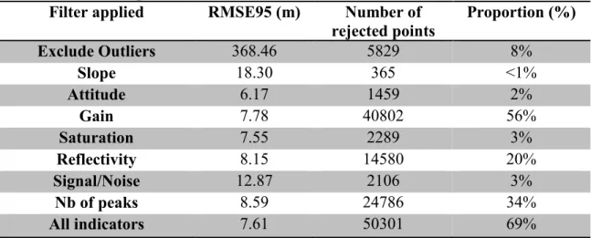
Table 3-2: Statistics on rejected points. The root mean square elevation error (RMSE95)
was calculated for points rejected for each filter of Table 3-1, with respect to the Canadian Digital Elevation Data (CDED) grid. The reference for the "Proportion (%)" is the initial number of points before exclusion of the outliers (72860).
Filter applied RMSE95 (m) Number of
rejected points Proportion (%)
Exclude Outliers 368.46 5829 8% Slope 18.30 365 <1% Attitude 6.17 1459 2% Gain 7.78 40802 56% Saturation 7.55 2289 3% Reflectivity 8.15 14580 20% Signal/Noise 12.87 2106 3% Nb of peaks 8.59 24786 34% All indicators 7.61 50301 69%
However, the rejection of so many points might have been a problem if the spatial distribution of the remaining points was rendered substantially sparser than the original dataset, anywhere in the AOI. Fortunately, this was not observed; the filtered points were still well spatially distributed even though they exhibited a lower density than the original tracks.
Exclusive filtering analysis
Results of the exclusive filtering are presented in Table 3-3 as a means of evaluating the pertinence of theindicators. It can be seen that the signal/noise and saturation indicators failed to exclusively filter elevation points. The signal to noise failure is related to the fact
25
that the gain is adjusted from the amplitude of the previous returned echoes (Zwally et
al., 2008) and the signal/noise is calculated using the maximum amplitude of the echoed
pulse: the same points are detected as potentially erroneous by both indicators. Therefore, they are redundant. However, since the gain indicator provides filtering results with a substantial decrease in root mean square error (Table 3-1) and showed a much broader capacity for point rejection (a substantially greater number of exclusively filtered points in Table 3-3), it appears more pertinent than the signal/noise indicator.
Concerning the saturation indicator, our analysis showed that the gain and the reflectivity indicators rejected most of the points that were initially rejected by this indicator. The reason is that the more aggressive constraining criteria of the reflectivity indicator supplanted the rejection criteria for saturated echoes. A high value of the gain indicator with, its attendant incitation of saturation in the face of rapid changes in surface reflectivity (see above) tended to complement, to a degree, the dominant rejection actions of the reflectivity indicator. Finally, the saturation points that were not rejected by the reflectivity and gain indicators were rejected by the indicator based on the number of peaks, without clear relationship between these processes. In this context, safely withdrawing the saturation indicator from the methodology presented in this paper requires further tests over other study sites.
Table 3-3: Proportion of points exclusively filtered out (rejected) by each indicator. The
number of points "exclusively filtered out" is the number of points retained after a 2nd filtering (of the rejected or filtered out points in Table 3-2) using a combined-indicator (all indicators but the one under evaluation) filter. The reference for the proportion column is the "Number of rejected points" column of Table 3-2.
Indicator Number of points exclusively rejected Proportion (%) Slope 329 90% Attitude 335 23% Gain 17136 42% Saturation 0 0% Reflectivity 1166 8% Signal/Noise 0 0% Nb of peaks 8427 23%