L'ADOPTION DEL' AGRICULTURE DE CONSERVATION AU BRÉSIL : CONSTRUCTION D'UN INDICE COMPOSITE POUR LES ÉTATS DE SANTA
CATARINA ET DU PARANA
MÉMOIRE PRÉSENTÉ
COMME EXIGENCE PARTIELLE
DE LA MAÎTRISE EN SCIENCES DE L'ENVIRONNEMENT
PAR
DIEGO CALLAC! TROTTIER
UNIVERSITÉ DU QUÉBEC À MONTRÉAL Service des bibliothèques
Avertissement
La diffusion de ce mémoire se fait dans le respect des droits de son auteur, qui a signé le formulaire Autorisation de reproduire et de diffuser un travail de recherche de cycles supérieurs (SDU-522 – Rév.07-2011). Cette autorisation stipule que «conformément à l’article 11 du Règlement no 8 des études de cycles supérieurs, [l’auteur] concède à l’Université du Québec à Montréal une licence non exclusive d’utilisation et de publication de la totalité ou d’une partie importante de [son] travail de recherche pour des fins pédagogiques et non commerciales. Plus précisément, [l’auteur] autorise l’Université du Québec à Montréal à reproduire, diffuser, prêter, distribuer ou vendre des copies de [son] travail de recherche à des fins non commerciales sur quelque support que ce soit, y compris l’Internet. Cette licence et cette autorisation n’entraînent pas une renonciation de [la] part [de l’auteur] à [ses] droits moraux ni à [ses] droits de propriété intellectuelle. Sauf entente contraire, [l’auteur] conserve la liberté de diffuser et de commercialiser ou non ce travail dont [il] possède un exemplaire.»
Je te dédie ce mémoire, Danièle Trottier, ma chère maman, mon ange qui est au ciel. C'est en suivant ton exemple de femme érudite que j'ai décidé de me lancer dans des études aux cycles supérieurs dans un domaine qui me passionne. Merci à toi aussi, Miguel Callaci, cher papa, qui m'a toujours appuyé et encouragé pendant mes études et durant la rédaction de ce mémoire.
Je tiens à remercier tout particulièrement mes directeurs de recherche, Charles Séguin et Marc Lucotte, de m'avoir offert l'opportunité de travailler sur ce projet. Votre amitié, vos connaissances et vos conseils et furent essentiels à la réussite de cette étape. Vous avez su guider ce travail avec excellence.
Un grand merci, également, au professeur Frédéric Mertens, qui m'a donné des judicieux conseils pour la préparation de mon terrain, ainsi qu'à tous ceux qui m'ont aidé à accomplir ma mission sur le terrain : Roni Ansolin et toute sa famille, Mirvane Chemin Manske, Ivonar Fontaniva, Johnny Bertocchi, Matheus Tonatto et sa famille, Cleoni Foppa, Rubem Silvério· de Oliveira Junior.
Je tiens aussi à remercier ma douce Marie-Hélène pour son amour, son appm inconditionnel et sa compréhension, qui m'ont aidé à tenir le coup du début jusqu'à la fin de ma rédaction. Et Lua pour la joie qu'elle apporte dans ma vie!
Et merci à tous ceux que j'ai croisés au PK-7515, et ayant fait partie de l'équipe pendant des périodes de temps variables : Sophie, Élise, Émile le pêcheur, Émile « Dion »,
Ill
Jérôme, Stéphane, Moema, Felipe, Rani, Florine, Francis, Matheus, Gabriel, et autres membres de l'équipe. Vous m'avez tous bien fait rire à un moment ou à un autre!
LISTE DES FIGURES ... vi
LISTE DES TABLEAUX ... vii
RÉSUMÉ ... viii
CHAPITRE I : INTRODUCTION GÉNÉRALE ... 9
CHAPITRE II: ADOPTION OF CONSERVATION AGRICULTURE IN BRAZIL: CONSTRUCTION OF A COMPOSITE INDEX FOR THE STATES OF PARANA AND SANTA CA TARIN A ... 16
Abstract ... 16
1. Introduction ... 17
2. Adoption concepts in· agriculture and their complexity ... 20
2.1 The compl_exity of analyzing the adoption of Conservation agriculture .. 20
2.2 Other explanations for the emergence of agricultural practices: the social practices theories ... 22
2.3 Previous analyses of the adoption of agricultural practices with composite indexes ... 23
3. Material and Methods .. · ... 25
3.1 Description of Study Sites ... 25
3.2 Data collection ... 27
3.3 Summary statistics ... 28
4. Building an Adoption of conservation agriculture index ... 31
4.1 The framework of the composite indicator ... 31
4.2 Selection of Conservation Agriculture indicators ... 32
4.3 Weighting scheme of the Adoption of Conservation Agriculture Index indicators ... 35
5. Results ... 37
5.1 Conservation agriculture practices of the sample group (before PCA) ... 37
5.2 Appropriateness of a principal component analysis ... .40
V
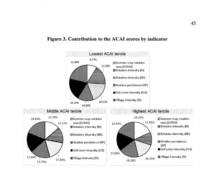
5.4 Contribution to the ACAI scores by indicator ... 44
5.5 Application of the separate and pooled regression models ... .46
5.6 Regional differences in ACAI scores ... .48
6. Discussion ... 49
6.1 Relationships between principal components ... 49
6.2 Separate and pooled regressions between the socio-economic variables and the ACAI ... 52
6.3 Summary and implications ... 53
7. Conclusion ... 55
CHAPITRE III : CONCLUSION GÉNÉRALE ... : ... 59
CONCLUSION GÉNÉRALE ... 59
Figure Page Figure 1. The number of interviews in each Rural Region in Parana and Santa
Catarina ... 26
Figure 2. Scree plot of the eigenvalues after the principal component analysis ... 41
Figure 3. Contribution to the ACAI by indicator ... .45
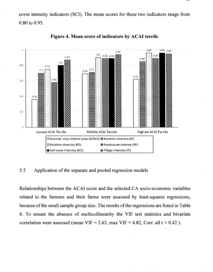
Figure 4. Mean score of ACAI indicators by tercile ... 46
LISTE DES TABLEAUX
Tableau Page
Table 1. Socio-economic variables of the sample group ... 29 Table 2. Comparison between selected variables of the sample group and state and
national level data (N=45) ... 30 Table 3 Evaluation parameters over a period (E;), benchmark values (B) and critical
indicator values. (Adapted from Roloff et al. (2011)) ... 35 Table 4. Conservation agriculture practices of the sample group ... 38 Table 5. PCA components used for Adoption of Conservation Agriculture Index
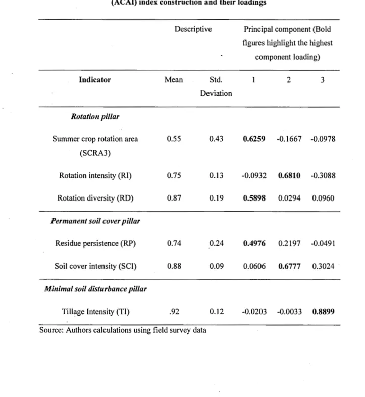
(ACAI) index construction and their loadings ... .43 Table 6. Separate regressions vs Pooled regression with ACAI and selected variables
À l'intérieur de cette recherche, nous construisons un indice d'adoption composite pour évaluer l'adoption de l'agriculture de conservation par des producteurs de soja et de maïs dans le sud du Brésil. Le niveau d'adoption des trois piliers de cette pratique, la rotation des cultures, la couverture permanente du sol, et sa perturbation minimale, est mesuré avec une série d'indicateurs notés sur une échelle de O à 1, et dont la pondération est établie grâce à une analyse en composantes principales. Un questionnaire d'entrevue, administré à vingt-neuf (29) producteurs de l'État de Santa Catarina et seize ( 16) producteurs de l'état du Paranâ, a été utilisé pour récolter les données auprès des répondants, identifiés grâce à la méthode d'échantillonnage non probabiliste de type « boule de neige ». Les analyses permettent de mettre en lumière trois éléments principaux: (1) l'intensité d'adoption de certains indicateurs reliés à la rotation des cultures et à la couverture permanente du sol, et plus particulièrement ceux qui mesurent la superficie de rotation des cultures d'été et la persistance des résidus, est plus faible, alors que l'indicateur attribué à la perturbation minimale du sol a des niveaux élevés d'adoption parmi tous les agriculteurs; (2) les producteurs appartenant à la région rurale de Maringâ obtiennent des notes plus faibles pour l'indice composite, ce qui suggère une configuration de marché moins favorable à la diversification des cultures dans cette région, mais aussi le rôle potentiel de la diversité géographique, susceptible de décourager l'apprentissage social et (3) l'indice composite d'adoption permet une mesure plus précise des trois composantes d'une pratique complexe comme l' AC, par rapport à une catégorisation binaire de l'adoption. Ces résultats exploratoires tendent à démontrer que l'adoption de l'agriculture de conservation dans le sud du Brésil est plus faible que ce qui est rapporté dans les statistiques officielles.
Mots-clés : adoption, agriculture de conservation, diversité géographique, indice
CHAPITRE I : INTRODUCTION GÉNÉRALE
Le semis direct est un système de culture sans-labour qui s'est popularisé dans les années 1970 au sud du Brésil, principalement pour lutter contre une érosion généralisée de la couche arable des sols dans les états du Parami, de Santa Catarina et de Rio Grande do Sul (Assunçào et al., 2013; de Freitas et Landers, 2014; Hogarth, 2017; Kassam et al., 2018). En partenariat avec les scientifiques, les producteurs agrièoles ont graduellement transformé la pratique du semis directs en un système, le système de semis directs (Sistema plantio direto, SPD), qui est aujourd'hui reconnu comme la version brésilienne de l'agriculture de conservation (AC). Il est basé sur trois principes interdépendants : l'absence, ou la moindre perturbation du sol à travers le semis-direct, la couverture permanente morte ou vivante du sol grâce au maintien d'une biomasse végétale, et la diversification des espèces végétales via la rotation et/ou la succession des cultures ( de Freitas et Landers, 2014; Kassam et al., 2018). Cela prit une vingtaine d'années, à partir de son introduction au pays, pour que le modèle atteigne une adoption significative ( de Frei tas et Landers, 2014 ).
Avec des niveaux supérieurs à 50 % dans les superficies de cultures annuelles (de Freitas et Landers, 2014), tels que rapportés par la FEBRAPDP (Fédération brésilienne de semis directs sous paillis), l'adoption de l'AC au Brésil est actuellement la plus grande en Amérique du sud et la seconde au niveau mondial, après celle.des États-Unis (Kassam et al., 2018; Lai, 2019). La superficie attribuée à cette pratique y était estimée, pour l'année agricole 2015/2016, à environ 32 millions d'hectares (Kassam et al.,
serait principalement cultivé en agriculture de conservation (Cattelan et Dall 'Agno!, 2018; Debiasi et al., 2015). Cependant, il est possible de remettre en question l'exactitude de ces chiffres puisque, selon Lande! (2015, p. 346), « Les chiffres estimant l'avancée du semis direct dans le pays sont sujets à caution, en raison du manque de données systématiques, du manque de partialité de certaines sources disponibles ( études produites par des acteurs faisant la promotion de l 'AC et/ou entretenant des relations de proximité avec les firmes d'agrofoumiture), et aussi de la diversité des techniques prises en compte indistinctement (semis direct sous couvert ou non)».
Or, si le Brésil, premier exportateur et le deuxième producteur mondial de grains de soja, est érigé en modèle de développement économique par certains, le système de production du soja brésilien est présenté par d'autres sous l'angle de ses conséquences sociales et écologiques considérables. Le pays occupe le premier rang mondial, depuis 2008, en termes de consommation de pesticides (Laval, 2015). L'adoption de systèmes d'AC est étroitement liée à l'utilisation généralisée des herbicides, car ils remplacent le travail du sol, un outil majeur de lutte contre les mauvaises herbes (Assunçào et al.,
2013; Cattelan et Dall'Agnol, 2018; Laurent et al., 2011; Palm et al., 2014). En raison de son climat tropical et des grandes surfaces cultivées, la production agricole brésilienne est confrontée à un défi majeur dans la lutte contre les ravageurs (Cattelan et Dall'Agnol, 2018). L'intensité de plusieurs problèmes phytosanitaires et de gestion des sols a augmenté : le compactage, l'infestation de mauvaises herbes difficiles à contrôler et même résistantes au glyphosate, et l'incidence de divers insectes ravageurs et maladies, parmi d'autres. Ces problèmes découlent en grande partie de la faible diversité des espèces cultivées dans les systèmes de production où le soja est présent (Debiasi et al., 2015; Salvadori et al., 2016).
11 L'adoption généralisée du modèle de l'agriculture de conservation au sud du Brésil est donc remise en question, puisque comme l'affirment Salvadori et al. (2016) et Denardin et al. (2012), la pratique du semis direct et l'agriculture de conservation sont deux concepts différents. Pour les conditions pédoclimatiques et climatiques de la région sud du Brésil, les deux principes du semis direct, qui sont la réduction ou l'élimination de la mobilisation du sol et l'entretien des résidus de culture dans le sol, sont insuffisants pour assurer la durabilité des cultures de grains annuelles. La consolidation des systèmes d'agriculture de conservation, d'autre part, repose essentiellement sur la diversification des cultures pour accroître la rentabilité, la promotion d'une couverture végétale permanente et la génération de bénéfices au niveau de la protection des plantes et du recyclage des nutriments. L'interaction entre la diversification des cultures, l'abandon du travail du sol et l'entretien d'un sol couvert en permanence assure l'amélioration progressive des caractéristiques biologiques, physiques et chimiques du sol. Les données sur l'adoption de l'agriculture de conservation au Brésil ont d'ailleurs été remises en question précédemment. Fuentes Llanillo et al. (2013) démontrent, par exemple, que les données de la Fédération brésilienne de semis direct sous paillis (FEBRAPDP) diffèrent de celles de l'Institut Brésilien de géographie et de statistique (IBGE). Alors que la FEBRAPDP déclarait une surface d'agriculture de conservation estimée à 25,6 millions d'hectares au Brésil en 2006, les données officielles de l'IBGE, basées sur le recensement de l'agriculture de 2006, faisaient plutôt état de 17,8 millions d'hectares de cette pratique dans les cultures annuelles.
La plupart des travaux s'étant penchés sur l'adoption de l'agriculture de conservation l'ont conceptualisée comme une distinction binaire, où l'agriculteur est classé comme adoptant ou non-adoptant à un moment spécifique (Higgins et al., 2019; Knowler,
2015). Cette façon de concevoir l'adoption s'applique, pourtant, assez mal à l'AC, puisqu'il s'agit d'une technologie complexe (Farooq et Siddique, 2015; Speratti et al.,
2015; Wall, 2007). Par conséquent, la mise au point, par la recherche et le conseil agricole, d'un modèle « universellement applicable » est presque impossible (Speratti
et al., 2015; Wall, 2007). D'autre part, l'abondante littérature sur l'adoption de l'agriculture de conservation n'offre pas vraiment de perspectives sur l'adoption ou l'abandon partiels de pratiques de l'agriculture de conservation (D'Souza et Mishra, 2018).
Dans cet ordre d'idées, quelques études (ITAIPU-BINACIONAL et FEBRAPDP, 2011; Martins et al., 2018; Roloff et al., 2011) ont utilisé, précédemment, un indice composite pour mesurer la qualité de l'agriculture de conservation, définie comme« la capacité d'un champ sans labour particulier à maintenir ou augmenter la productivité . des cultures et du bétail tout en maintenant ou en améliorant la qualité du sol, de l'eau et de l'air et les autres services environnementaux» (Roloff et al., 2011, p. 1) dans des régions spécifiques du Brésil. Bien qu'elles utilisent toutes le même indice composite, le No-Till Systems Quality Index (NTSQJ), pour évaluer la qualité des systèmes d'agriculture de conservation plutôt que leur adoption, quelques aspects de ces recherches doivent être soulignés. D'abord, la définition de l'agriculture de çonservation, des composantes à intégrer, et des seuils à partir desquels les composantes sont considérées comme ayant une bonne qualité, a été effectué dans une dynamique collaborative, à travers des ateliers intégrant de nombreuses parties prenantes et permettant aux agriculteurs locaux de donner leur opinion sur la composition de l'indice de qualité, tel que décrit par ITAIPU-BINACIONAL et FEBRAPDP (2011). De plus, l'indice permet d'évaluer la qualité des trois piliers de l'agriculture de conservation, la rotation des cultures, le maintien d'une couverture
13 végétale permanente et la perturbation minimale du sol, à travers une série de 4 indicateurs. 4 autres indicateurs servent à évaluer la qualité des pratiques de conservation du sol à travers la fréquence des débordements et des épisodes érosifs, la compaction du sol dans la propriété en général, les sources d'engrais et le nombre d'années d'utilisation de la pratique du semis direct sur la propriété. D'autre part, l'indice composite utilisé dans ces travaux considère l'aspect multi saisonnier de la rotation des cultures, puisque l'évaluation effectuée à travers cet indice est basée sur un cycle de 3 ans de cultures. Enfin, bien que défini d'une façon subjective, le système de pondération attribue un poids important (1,5 points sur une échelle de 10) à chacun des 4 indicateurs directement reliés aux piliers de l'agriculture de conservation, attribuant ainsi un poids important (45% du poids de l'indice) aux 3 indicateurs reliés directement ou indirectement à la rotation des cultures. Ces études précédentes utilisaient donc un indice composite pour évaluer la qualité de l'agriculture de conservation chez des producteurs brésiliens, mais à notre connaissance, notre recherche est la première à mesurer le niveau d'adoption de l'agriculture de conservation des ménages agricoles par le biais d'un indice composite dont les-indicateurs sont pondérés grâce à une méthode statistique, celle de l'analyse en principales composantes. Cette méthode permet, entre autres, d'accorder un poids plus important aux indicateurs pour lesquels les résultats obtenus ont une plus grande variabilité.
La chaire de recherche à laquelle je me suis joint, dirigée par le pràfesseur Marc Lucotte, étudie la transition vers la durabilité des grandes cultures et les conséquences environnementales de l'utilisation des herbicides à base de glyphosate depuis plusieurs années. Bien que l'apparition de nouvelles molécules herbicides ait été un facteur déterminant dans l'adoption de l'agriculture de conservation à grande-échelle
(Assunçào et al., 2013; Hogarth, 2017), cette recherche ne vise pas à approfondir ce sujet. L'objectif principal de mon projet de recherche était plutôt de caractériser l'adoption de l'agriculture de conservation. Le terrain a été réalisé dans le sud du Brésil afin de mieux comprendre le niveau d'adoption de cette pratique chez des producteurs de grandes cultures de cette région du monde, ainsi que les raisons pour lesquelles ils adoptent ou abandonnent la pratique. Cela a abouti en la production d'un article intitulé
«
Adoption of Conservation Agriculture in Brazil: Construction of a composite index for the States of Parana and Santa Catarina », co-écrit par Charles Séguin, Marc Lu cotte et Rubem Silvério de Oliveira Junior. Ce dernier constitue le prochain chapitre de ce présent mémoire et sera soumis pour publication dans la revue Ecological Economies. L'instrument de collecte de données utilisé consistait en un questionnaire d'entrevue que j'ai élaboré, et qui a été révisé et validé par deux agronomes de l'ouest de Santa Catarina et testé auprès d'un producteur de grandes cultures de cette même région. Il comportait des questions fermées et d'autres qui étaient ouvertes et semi-dirigées, permettant ainsi aux producteurs d'offrir une réponse sans choix prédéterminés. Ce questionnaire a permis de collecter des données socio-démographiques sur les participants et leurs exploitations, ainsi que sur leurs pratiques agricoles et leurs perceptions sur l'agriculture de conservation. Le premier auteur de l'étude a conduit les entrevues, compilé les données collectées auprès des producteurs agricoles, et procédé à des analyses statistiques et à l'interprétation des résultats obtenus. Les co-auteurs ont supervisé l'échantillonnage sur le terrain et les analyses statistiques et ont révisé le texte.Cette étude a été financée grâce à une bourse octroyée par le Ministère des affaires étrangères, du commerce et du développement du Canada. De plus, quelques
15 partenaires ont été importants dans la sélection du terrain de recherche et de ses participants, notamment !'Entreprise SEMA TTER de Sào Miguel do Oeste et l'Université d'État de Maringa (UEM). La région du sud du Brésil a également été choisie pour cette étude en raison des contradictions entourant l'adoption généralisée de l'AC. Alors que pour certains auteurs, le niveau d'adoption déclaré de l'agriculture de conservation dans cette région est proche de 100% (Kassam et al., 2018), et que, dans les États du sud du Brésil, l'agriculture de conservation est la norme (de Frehas et Landers, 2014 ), d'autres auteurs affirment que c'est le semis direct, qui respecte uniquement deux piliers de l'agriculture de conservation sans intégrer la diversification des espèces végétales, qui domine la région (Salvadori et al., 2016). Nous avons mené des entrevues dans quatre régions rurales du sud du Brésil, deux dans l'État de Santa Catarina et deux dans l'État du Parana.
Le prochain chapitre de ce mémoire consiste en l'article scientifique, dans lequel on retrouve la problématique et l'objectif de recherche, les matériels et méthodes, les résultats, la discussion et la conclusion. Le dernier chapitre fait office de conclusion générale du mémoire.
AND SANTA CATARINA
Diego Callaci Trottier, Charles Séguin, Marc Lucotte, and Rubem Silvério de Oliveira Junior
Abstract
Conservation Agriculture is a crop production system characterized by minimal soil disturbance, permanent soil cover and crop rotations. The analysis attempts to assess the degree of adoption of Conservation Agriculture and its dimensions at the farm lev el of 45 field crop farmers (soybean and maize) in the states of Santa Catarina and Paranâ, southern BraziLWe developed a composite index of Conservation agriculture using a principal component analysis based weighting scheme. Separate and pooled regression models were also applied to verify the relationship between the index and socioeconomic variables related to the farmers and their farms. The empirical results show that the intensity of adoption of some indicators related to crop rotations and permanent soil cover is lower, especially those measuring the area of the summer crop rotation and the persistence of the crop residues, while the minimal soil disturbance indicator has high levels of adoption amongst ail farmers; that belonging to the Rural Region of Maringâ is negatively correlated with the Adoption of Conservation Agriculture Index; and that we can better characterize the diversity of Conservation Agriculture practices with our composite index than with a binary measure of adoption. As this is an exploratory study with a convenience sample, our results are hardly generalizable, but they are consistent with previous findings suggesting that the levels of Conservation Agriculture adoption in southern Brazil are lower than those officially reported, as some farmers are not adopting fondamental pillars of the practice such as crop diversification.
Keywords: Adoption, Conservation agriculture, Southern Brazil, Composite index, Principal component analysis, Soybean, Rotations
1. Introduction
Conservation Agriculture (CA) is a crop production system characterized by three interlinked principles, namely: minimal soil disturbance, a permanent living or dead soil cover and crop rotations. Authorities worldwide reported that it was practiced on about 180 M ha (12.5% of global cropland) in 2015/2016. With levels above 50%, CA adoption is among the highest in the world in the southem parts of South America. Brazil possesses one of the largest CA areas in the world with an estimation of 32 M ha of CA in the 2015/2016 crop year (Kassam et al., 2018). Brazilian soybeans are grown mainly under no-till systems (Cattelan and Dall'Agnol, 2018; Debiasi et al.,
2015), a term employed for Brazilian CA. A variety of names such as the no-tillage system (Fuentes-Llanillo et al., 2018), direct seeding mulch-based cropping systems (DMC) (Alary et al., 2016), direct planting system (Assunçao et al., 2013) or Zero Tillage Conservation Agriculture (ZT/CA) (de Freitas and Landers, 2014) have been used to refer to this practice. They all represent the Brazilian version of CA. To avoid confusion, we retain the term of CA for this paper.
Erected as a model of economic development by some, the soybean production system of the world's largest exporter and the second-largest producer of this commodity has several significant social and ecological consequences. Since 2008, Brazil has been ranked first in the world in terms of pesticide consumption (Laval, 2015). The adoption of CA systems is closely related to the widespread use of herbicides because they replace the use of tillage, a major tool for controlling weeds (Assunçao et al., 2013; Cattelan and Dall' Agnol, 2018; Laurent et al., 2011; Palm et al., 2014). In addition, because of its tropical climate and the large cultivated areas, the country faces a major challenge in controlling pests that affect agricultural production (Cattelan and Dall'Agnol, 2018). Severa! phytosanitary and soil management problems have increased in intensity, such as soil compaction, the infestation ofweeds that are difficult
to contrai and sometimes even resistant to herbicides, and havoc of various insect pests and diseases. To a large extent, these issues arise from the low diversity of species cultivated in soybean production systems (Debiasi et al., 2015).
Thus, there are serious concerns about the quality of some CA systems. Despite systematically applying the no-till practice, a significant number of farmers are opting for soy mono-cropping, and/or with no living or dead plant cover between cash crops (Kassam et al., 2018). In many fields, the pillars of the crop rotation and the maintenance of a constantly covered soil have been neglected. These management practices have promoted setbacks in soil conservation in recent years. As an example, in the state of Rio Grande do Sul, there is a graduai return of erosion in annual grain crops, associated with changes in the physical, chemical and biological properties of the soil, which compromises the stability of the production system (Barbieri et al.,
2019). These observations are in line with previous findings on the Brazilian CA situation. For example, according to Denardin et al. (2008), for most of the annual grain crops in the states of Rio Grande do Sul and Santa Catarina, the no-till system was not being adopted and conducted in accordance with the minimum recommendations that made it viable as a CA tool in Brazil. Bolliger et al. (2006) also found that many smallholder farmers only partially adopt some CA practices, rather than respecting the full principles of this cropping system.
ln this paper, we measure the farm household level of adoption of Conservation
Agriculture by the development of a composite index, the Adoption of Conservation Agriculture Index (ACAI), and use a principal component analysis to weight its indicators. A composite index is formed by individual indicators, on the basis of an underlying model, to measure a multi-dimensional concept that cannot be captured by a single indicator (OECD, 2008). This index contributes to understanding the patterns of the adoption of the three conservation agriculture pillars at the farm-level, in four Rural Regions of the two southern Brazil states of Paranâ and Santa Catarina, where
19
we conducted interviews with 45 soybean and maize producers. With a 3-year assessment, we were able to capture the multi-seasonal dimension of crop rotations. Using a selection of independent variables in separate and pooled linear regression models, we found a strong negative relationship between the composite index and the Maringâ Rural region of belonging, suggesting a possible influence from the different soi! composition of this region. Finally, we compare the composite index of adoption to the more traditional binary measure and conclude that such a continuous measure can better characterize the degree and the heterogeneity of CA adoption than a binary one. This is an exploratory study with a convenience sample; therefore, the results are not generalizable to al! Brazilian producers, nor to th ose in the states of Paranâ or Santa Catarina.
This paper is organized into seven sections. In section two, we present the basic concepts of adoption used to analyze technological change and justify the need to go beyond a binary scheme of adoption (2.1). We also explore the social practice theories and their usefulness in explaining the adoption of agricultural practices (2.2). Then, we describe previous studies that analyze agricultural practices with a composite index (2.3). In section three, we describe the study site (3.1) the data collection (3.2) and the data (3.3). In section four, we explain how our composite index was built. First (4.1), we describe the framework on which our composite indicator is based; then (4.2), we specify how our indicators were selected and (4.3) how their respective weights are defined. In section five, we schematize the results, which are discussed in section six. Research conclusions and their implications for the theory and practice on conservation agriculture adoption are presented in section seven.
2. Adoption concepts in agriculture and their complexity
2.1 The complexity of analyzing the adoption of Conservation agriculture
The study of technical change in agriculture in developing countries has often been analyzed through the lenses of the concept of adoption. On one hand, there is the individual (farm-level) adoption, while on the other, aggregate adoption (regional or national level) is usually referred to as diffusion. But there are two problems underpinning the idea that was used in much of the literature of CA adoption. The first is a conception oftechnology as discrete, generic and transferable packages of material and practical packages; the second is a relatively simple, largely individual, dichotomous yes/no, once-and~for-all and linear perception of technological change (Glover et al., 2016). In most agricultural adoption research, the former is classified as an adopter or non-adopter at a single point intime (Foguesatto and Machado Dessimon, 2019; Knowler, 2015; Place and Swallow, 2000). Much of the previous work on the adoption of conservation agriculture has conceptualized it as a binary distinction (Glover et al., 2016; Higgins et al., 2019; Jaïn et al., 2009; Knowler, 2015). In the case of a single technology such as a crop variety, it can be measured as the proportion of the land per unit of cropped area where it is applied: this notion is known as the intensity of adoption (Glover et al., 2016; Jaïn et al., 2009). But measuring the adoption becomes more difficult in the case of a blend of agricultural technologies, (Jaïn et al., 2009). CA is a complex technology (Farooq and Siddique, 2015; Speratti et al., 2015; Wall, 2007) that includes a set of practices such as wise soi! manipulation, keeping crop residues onsite, planned and diversified crop sequences, and effective weed management (Farooq and Siddique, 2015). Therefore, the development of an appropriate "one size fits all" CA package by the research and the agricultural extension services is almost impossible (Wall, 2007). The literature on CA adoption is extensive, but it often fails
21
to offer insights on the adoption and abandonment of partial conservation agriculture technologies or practices (D'Souza and Mishra, 2018).
CA practices are knowledge-intensive and imply a complete change in the farming system management {Speratti et al., 2015), which means that the adoption process is ongoing and complex. Farmers use their tacit knowledge, practical skills and previous farming experience to define what combinations of practices or techniques are likely to be most relevant and effective in their situation, to ensure the ongoing economic and social viability of their farm. They do not simply follow a rigid, pre-formatted set of rules and procedures in the implementation of farming techniques (Higgins et al.,
2019). They may adopt some CA principles white maintaining a degree of flexibility in their approach. Thus, the decision exceeds any simple binary classification as a choice to adopt or not to adopt, because the farmers face a set of technology options. More realistically, the decision may involve selecting from several options or 'packages' among which not to adopt is just one of these multiple alternatives (Higgins
et al., 2019; Knowler, 2015).
On the other hand, adopting new agricultural practices is a dynamic process and should include the time dimension. Nevertheless, most studies are cross-sectional and consider only a single point in time. However, considering the timing of the decision to adopt can be as important to understand as the decision itself (Knowler, 2015). Moreover, adoption estimates often do not consider the number of cropping seasons in which CA practices have been applied. However, the third CA principle, crop rotation, requires a multi-seasonal definition of adoption. Although the CA definition used in different countries usually defines crop rotation as a sequence of three crops (Andersson and D'Souza, 2014), it might not be the case for South American agricultural systems. In Brazilian CA systems, a crop succession, on one hand, consists of the arrangement of two crops in the same agricultural area for an indefinite period of time, each cultivated in a given season of the year (Debiasi et al., 2015; Franchini et al., 2011). On the other
hand, a crop rotation is defined "as the orderly altemation of different crops, in a given time frame (cycle), in the same area and in the same season of the year" (Debiasi et al.,
_2015; Franchini et al., 2011) or "consisting of the orderly altemation of different crops in a time frame and in the same area, where a plant species is not repeated in the same place in a time frame of less than one year" (Barbieri et al., 2019; EMBRAPA, 2013). In both cases, the definition requires a multi-seasonal approach to assess crop rotations from one year to another.
2.2 Other explanations for the emergence of agricultural practices: the social practices theories
In the same vein, some theories put forward alternative narratives to explain the practices implemented by the farmers. In particular, the social practice theories have analysed how social practices emerge and become "normal" practices, instead of focusing on behavior change (Roysen and Mertens, 2019), and placed "emphasis on discourses and . actions which make up practices in specific sociocultural contexts"(Sahakian et al., 2017, p. 509). In addition, according to these theories, "practices can only emerge, persist or change when connections between certain elements are made, sustained or broken" (Roysen and Mertens, 2019, p. 2). They consider that practices are not only the result of rational decisions of the actors but that they depend on three categories of factors: 1) the meanings of the practices in place (what does it mean, for example, to cover the soil for farmers, rather than leaving it uncovered? What are the standards that promote the maintenance or evolution of practices? Etc.); 2) the available materials (what are the instruments, infrastructures, agricultural products that determine practices and/or allow the emergence of new praètices? Etc.); 3) the competences (what knowledge and skills are needed to change practices, what are the leaming contexts? Etc.)(Roysen and Mertens, 2019; Sahakian
et al., 2017; Shove et al., 2015). These three categories are interlinked to form an integrated and coordinated chain of routine and habit, and, as a consequence, the social
23
practices change when the connections between these elements change (Roysen and Mertens, 2019). Analyzing the conservation agriculture-related practices through the lens of these theories is out of the scope of this paper, but these approaches should be highlighted as likely to provide additional or alternative explanations to the adoption of new agricultural practices.
2.3 Previous analyses of the adoption of agricultural practices with composite indexes
Previous studies have evaluated the adoption of agricultural practices through a composite index with a weighting system. Sorne ofthem derived the weighting system from principal component analysis. In particular, Mutabazi et al. (2015) constructed a composite index of resilience-building adaptive strategies (REBAS) of farm households, based on a set of selected indicators, to assess the adoption of resilience-building measures. With the PCA, they reveal the latent structure and internai correlations among different classes of adaptive strategies and generate scores used as weights in the construction oftheir index. They also apply a multiple regression model to study the relationship between the REBAS index and four types of capital (human, financial, natural and societal), revealing that faith in climate change as anthropogenic phenomena is the key human câpi~al variable influencing the resilience-building strategies. In a similar way, Li et al. (2016) develop a composite index to evaluate the sustainability of farm households using a weighting scheme based on a principal component analysis. They also use multiple regression models to understand how the environmental, economic and social dimensions oftheir farm household sustainability (FHS) composite index are driven by seven categories of determinants, i.e. knowledge, demographics, economics, technology, settlement type, land use, and level of social participation. They conclude that the share of the area of set-aside land through the Grain for Green Program (GGP) as a proportion of the total farmland proved to be the key determinant of agricultural _sustainability.
Jaïn et al. (2009) measure the adoption of improved cultivation practices by the development of a state-wise composite index, to conclude with a highly significant correlation between the latter and the state-wise agricultural productivity. However, if they also assess the determinants of the adoption index with a multiple regression model, they do not integrate a principal component analysis in their study.
In addition, other studies (ITAIPU-BINACIONAL and FEBRAPDP, 2011; Martins et al., 2018; Roloff et al., 2011) have already used a composite No-Till Systems Quality Index (NTSQI) with a multi-seasonal approach of crop rotations (3 crop years) to assess the quality of Brazilian CA, defined as" the capacity of a given no-till field to main tain or increase crop and livestock productivity while maintaining or enhancing soi!, water and air quality and other environmental services" (Roi off et al., 2011, p. 1 ). The study conducted by ITAIPU-BINACIONAL and FEBRAPDP (2011) assessed the quality of CA of 25 producers with · the composite index, and the results presented a good amplitude, ranging from 4.8 to 9.7 on a scale of O to 10, which led the authors to conclude that the index was able to clearly differentiate between the No-Till practices of the farmers. The indicator with the highest frequency of critical cases (52%), Terrace adequacy (TA) was related to the proper terrace management. The other indicators that appeared to be critical, in 32% of the cases, were related to the diversity of crops in the rotation scheme (Rotation diversity - RD) and the persistence of the crop residues (Residue persistence - RP), both related to the assessment of the crop rotation pillar of CA. The results from Roloff et al. (2011) were, similarly, from a sample of24 farmers, and the values obtained for the composite index ranged from just below 6 to near 9, on the same scale. The two most critical indicators were TA (54% of the sample) and RP (29% of the sample ), which led the authors to conclude "that actions aimed at improving NTS quality for those farmers must focus on terrace adequacy and on increasing the number of grass cover crops in the rotation, by using winter cover crops such as black oats" (Roloff et al., 2011, p. 2). In the study of Martins et al. (2018), the ex-ante phase-field study had a similar sample size, with 19 producers from 12 different
25
watersheds in 5 states of Brazil: Sao Paulo, Mato Grosso do Sul, Goias, Parana, and Rio Grande do Sul. The results from their study also show critical values for the average scores of the RD (0,67 out of 1,00) and the RP (0,50 out of 1,00) indicators obtained by the farmers from the Rolândia and Cambé regions in Parana. These previous studies used a composite index to assess the quality of conservation agriculture, but to the best of our knowledge, our research is the first to measure the farm household level of adoption of conservation agriculture with a composite index by using indicators weighted through a principal component analysis.
3. Material and Metbods
3.1 Description of Study Sites
The Southern Brazil region was chosen for this study because of the widely reported adoption of CA and the controversy surrounding it. The declared adoption level of CA farming in this region is close to 100% (Kassam et al., 2018). In the southern states of Brazil, the practice of no-till conservation agriculture is presented as the norm ( de Freitas and Landers, 2014) but some authors have doubts about these figures (Bolliger
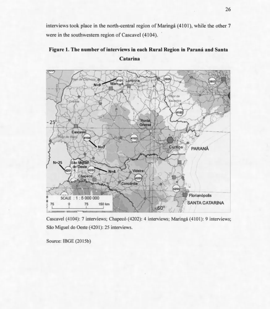
et al., 2006; Denardin et al., 2008; Fuentes Llanillo et al., 2013; Landel, 2015). We conducted 45 baseline field interviews in four Rural Regions, two in the State of Santa Catarina and two in the state of Parana. The geographical delimitation of the Rural Regions is based on the regional geographic differences as well as municipal contiguity, but also on the economic flows of the main agricultural products (IBGE, 2015a). In Figure 1, it is possible to see the geographical location of the regions from which respondents corne, as well as the number of respondents from each region. 25 interviews were conducted in the Rural Region ofSao Miguel do Oeste (4201) and four (4) in Chapec6 (4202), in the west of Santa Catarina state. In the state of Parana, 9
interviews took place in the north-central region of Maringa (4101), while the other 7 were in the southwestern region of Cascavel ( 4104 ).
Figure 1. The number of interviews in each Rural Region in Paranâ and Santa Catarina 11 Il
t
75 ·o )J,,- l f ... l~~ ;;}l!!i.- ~- ·- - ___ _ 75Cascavel (4104): 7 interviews; Chapec6 (4202): 4 interviews; Maringa (4101): 9 interviews; Sao Miguel do Oeste ( 4201 ): 25 interviews.
27
3.2 Data collection
The target population for this study was soybean and corn growers. 45 interviews were conducted during the period between September and December 2017 .1 A nonprobability snowball sampling method was used to identify respondents because information about them was not easily accessible and the area was difficult to reach. This technique involves the use of a known contact who identifies other persons to be considered as study participants (Kaweesa et al., 2018). The starting point was the cover crops specialized enterprise, SEMA TTER, established in the city of Sao Miguel do Oeste, Santa Catarina, identified with the help of a CA specialist from Quebec, Canada. An agronomist of SEMA TTER, in turn, identified soybeans and corn farmers. Respondents were asked to refer other potential study participants, and other agronomists referred by SEMA TTER also helped the researchers to reach the first 36 farmers, both from Santa Catarina and Parami states. Subsequently, a Weed Science professor at the State University of Maringâ (UEM) helped to reach 9 additional soybean and corn growers.
The administration of an interview questionnaire was the method used to collect data from farmers. The questionnaire, containing close-ended, multiple-choice and open-ended questions, was organized under different sections, to collect information on the socio-economical characteristics of the property administrator, the agricultural practices, and the vision of conservation agriculture. The interviews were conducted in the presence of the agronomists or the Weed Science professor, who helped to ensure that the questions had been well understood by the interviewees and duly been responded. Data was initially entered in Excel sheets before analysis using Stata software version 15.
1 Ail the farmers voluntarily agreed to speak with us and signed a consent forrn approved by the UQAM Research Ethics Committee (CERPE).
3.3 Summary statistics
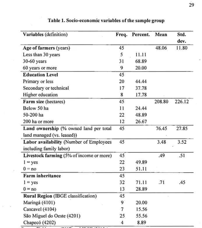
The statistics on the respondent farmers and their farms are listed in Table 1. As this is an exploratory study, we should be cautious in generalizing the results. Moreover, the latter are difficult to extrapolate to the general population because of the differences observed between the sample and the study population, which will be described in the following text. As far as farm attributes are concemed, we observe that the average percentage of cultivated land being leased to another owner is 24% and that more than half (51%) of the producers raise livestock for profit (representing at least 5% oftheir income). There is also a large variation in labor availability, as the average of 3,48 employees per farm is lower than the ~tandard deviation of 3,52.
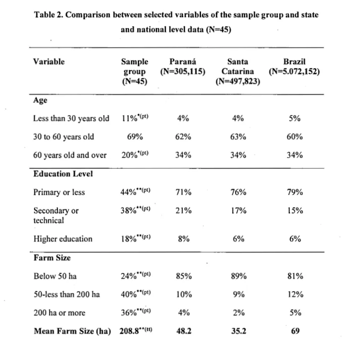
Table 2 presents a set of selected characteristics, for which the Brazilian national and state-level data was available. When comparing the characteristics of the field crop producers of the sample group and their farms to the data from the 2017 agricultural census from the Brazilian Institute of Geography and Statistics (IBGE, 2017a), we observe differences in the age distribution (Table 2). The producers interviewed, men only, are on average 48 years old, which is a little bit older, but very close to the national average age (46,5 years old) of rural producers (ABMRA, 2017). However, the proportion of producers under 30 years of age is 11 %, while the producers in this category represent only 4% in both states, and 5% at the national level. The proportion test shows that the percentages differences between the sample group and the IBGE data for this age category are statistically significant (0.05 significance level). The same test shows no statistically significant difference for the 30 to less than 60 years old age category. Lastly, there is a statistically significant difference (0.05 level) between the 60 years old and over category of Santa Catarina, Paranâ, and Brazil, where they represent more than a third of the producers' population (34%), and the sample group where they are 20%.
29
Table 1. Socio-economic variables of the sample group
Variables (definition) Freq. Percent. Mean Std.
dev.
Age of farmers (years) 45 48.06 11.80
Less than 30 years 5 11.11
30-60 years 31 68.89 60 years or more 9 20.00 Education Level 45 Primary or less 20 44.44 Secondary or technical 17 37.78 Higher education 8 17.78
Farm size (hectares) 45 208.80 226.12
Below 50 ha 11 24.44
50-200 ha 22 48.89
200 ha or more 12 26.67
Land ownership (% owned land per total 45 76.45 27.85
land managed (vs. leased))
Labor availability (Number of Employees 45 3.48 3.52
including family labor)
Livestock farming (5% ofincome or more) 45 .49 .51
1 =yes 22 49.89
0=no 23 51.11
Farm inheritance 45
1 = yes 32 71.11 .71 .45
0=no 13 28.89
Rural Region (IBGE classification) 45
Maringâ (4101) 9 20.00
Cascavel ( 4104) 7 15.56
Sao Miguel do Oeste ( 4201) 25 55.56
Chapec6 ( 4202) 4 8.89
Table 2. Comparison between selected variables of the sample group and state and national level data (N=45)
Variable Sample Parami Santa Brazil
group (N=305,115) Catarina (N=S.072,152)
(N=45) (N=497,823)
Age
Less than 30 years old 11 %*(pt) 4% 4% 5%
30 to 60 years old 69% 62% 63% 60%
60 years old and over 20%*(pt) 34% 34% 34%
Education Level Primary or less 44%**(pt) 71% 76% 79% Secondary or 38%**(pt) 21% 17% 15% technical Higher education 18%**(pt) 8% 6% 6% Farm Size Below 50 ha 24%**(pt) 85% 89% 81% 50-less than 200 ha 40%**(pt) 10% 9% 12% 200 ha or more 36%**(pt) 4% 2% 5%
Mean Farm Size (ha) 208.S**(tt) 48.2 35.2 69
*, * *
=
0.05 and 0.01 significance levels, respectively, for the one-sample test of proportion (pt) and the one-sample t-test (tt)31
The average education level of producers interviewed in this study is also higher than that of producers in the states of Santa Catarina and Paranâ, and Brazil. While the distribution shows that most producers have a Primary level or less (70% for both states and 79% at the national level), the proportion of this category is 44% for the sample group. 56% of the sample group has at least a secondary level of education, while it is less than 30% for Brazil, Paranâ, and Santa Catarina. All these proportions differences are statistically significant at a 0.01 significance level. lt should also be noted that in our sample, the younger farmers had a higher level of education. The 5 producers who were 30 year old or younger all had, at least, a secondary or technical level of education. Among the 31 sample farmers that were in the 30 to 60 years old category, most of them (14) had a secondary or technical level of education, while almost the same number (12) were below and only 5 of them had a higher education degree. And eight of the nine farmers above 60 years of age had only reached a primary lev el of education or below, whereas only one of them had a secondary or technical level of education.
There are also significant differences (at 0.01 level) in farm size. The farms below 50 ha represent 24% of the sample group, while in the two Brazilian states and in the whole country, they constitute over 80% of the farms. The farms between 50 and 200 ha and larger than 200 ha are overrepresented in the study, as they count for 76% of the sample group, while these combined categories are less than 18% at all the other geographic scales. The results of the one-sample t-test, used to test the null hypothesis that the population mean is equal to the ones retrieved from IBGE data, also show a statistically significant difference between the mean farm size of the sample group (209 ha) and the state-level and national values.
4. Building an Adoption of conservation agriculture index 4.1 The framework of the composite indicator
We focus on the adoption of conservation agriculture at the farm household scale to develop an ex-post assessment of the CA adoption of farms. In order to identify the indicators capturing the essence of conservation agriculture at the farm level, we applied a framework inspired by the No-Till Systems Quality Index {NTSQI) by ITAIPU-BINACIONAL and FEBRAPDP (2011) and Roloff et al. (2011). Based on this framework, we chose to build a composite "Adoption of Conservation Agriculture Index" (ACAI), as a composite indicator "should ideally measure multidimensional concepts which cannot be captured by a single indicator" (OECD, 2008, p. 13) like Conservation agriculture, a complex technology (Farooq and Siddique, 2015; Speratti
et al., 2015; Wall, 2007). Sorne of the benefits of the composite indicators include: that they can summarise complex, multi-dimensional realities with a view to supporting decision-makers; that they are easier to interpret than a battery of many separate indicators; that the reduce the visible size of a set of indicators without dropping the underlying information; and that they enable users to compare complex dimensions effectively. It should be noted, however, that there may also be disadvantages associated with the use of composite indicators, such as the fact that they can send misleading policy messages if they are poorly constructed or misinterpreted; that they may be misused if the construction process is not transparent or if it lacks sound statistical or conceptual principles; that the selection of indicators and weights could be the subject of political dispute; and that they may disguise serious failings in some dimensions and increase the difficulty of identifying proper remedial action, if the construction process is not transparent, among other disadvantages (OECD, 2008).
4.2 Selection of Conservation Agriculture indicators
Here the three pillars of CA, namely minimal soil disturbance, a permanent living or dead soil cover and crop rotations, as defined by many authors (Kassam et al., 2018; Kaweesa et al., 2018; Knowler and Bradshaw, 2007; Lemken et al., 2017; Palm et al.,
33
2014; Panne Il et al., 2014; Speratti et al., 2015) are represented by a set of six key indicators presented below, to .reflect these pillars directly or indirectly in a simitar manner to ITAIPU-BINACIONAL and FEBRAPDP (2011) and Roloff et al. (2011). They are selected based on their specificity and relevance in the study area and the availability of data, and the objective of this approach was also to represent these pillars of CA adoption with a minimum number of indicators. A fourth component used by ITAIPU-BINACIONAL and FEBRAPDP (2011) and Roloff et al. (2011) to evaluate an off-site outcome, was previously addressed by the evaluation of terrace adequacy (TA), assessed by the run-off over-topping frequency, and conservation evaluation (CE), based on the absence of signs of erosive run-off. As our goal was to assess the adoption and not the quality of the Brazilian no-till systems, we kept the indicators used to reflect the three CA pillars and did not integrate the run-off component indicators, nor the indicators previously used to assess plant nutrition (BN) or the time of adoption of no-till (AT), as it was done elsewhere (IT AIPU-BINACIONAL and FEBRAPDP, 2011; Roloff et al., 2011 ).
The crop rotation pillar is evaluated through the rotation intensity (RI) and rotation diversity (RD) indicators that were kept from the assessments of 1T AIPU-BINACIONAL and FEBRAPDP (2011) and Roloff et al. (2011 ). An indicator that was not included in previous studies, the summer crop rotation area (SCRA3), was also used to measure this CA pillar. Soi! cover permanence is assessed by the crop residue persistence (RP), and soi! cover intensity (SCI). In the original NTSQI used by ITAIPU-BINACIONAL and FEBRAPDP (2011) and Roloff et al. (2011), the RP indicator was related to the crop rotations pillar, but the choice to use it to assess the permanent soit cover dimension was based on the fact that this indicator also measures the soit cover permanence through the number of grass cover crops used in the rotation. For the SCI indicator, it is a modified version of the rotation intensity (RI) indicator used in the study of Martins et al. (2018), also based on the NTSQI index, where they replaced the original RI indicator by this one, which evaluates the number of months
covered by living plants in the 3 years reference period; thus, for our study, it was used as an indicator of the permanent soil cover dimension of CA. The minimal sàil disturbance is assessed by tillage intensity (TI), which calculates, in percentage, the average area not tilled in the past 3 years, instead of the previous indicator used by ITAIPU-BINACIONAL and FEBRAPDP (2011) and Roloff et al. (2011), tillage frequency (TF), which calculated the proportion, in years, between the number of years without tillage compared to the time considered ideal for stabilizing the system. Ali indicators are determined for a 3-year period, arguably easily remembered by farmers (ITAIPU-BINACIONAL and FEBRAPDP, 2011; Roloff et al., 2011).
The value of each indicator (Ji) based on a benchmark is calculated as described in Equations (1 ):
Ei
Ii=B (1)
where E; is a present or future value of a field parameter for farm i and B is a regional benchmark value suggested by experimental results or expert opinion, as is the case with critical values, in the NTQSI framework (ITAIPU-BINACIONAL and FEBRAPDP, 2011; Roloff et al., 2011). We used the benchmarks and critical values previously defined in the original NTQSI for the indicators we kept in our study (Table 3), as the original research was also conducted with farmers from southem Brazil Rural regions. Through our field observations with the 45 producers interviewed, it was defined that these values could be applied to our study, because of the similarity between farm household agricultural systems concemed by both studies. However, the authors of the original framework used, as explained in Roloff et al. (2011, p. 2) a "subjective weighting factor used to emphasize some indicators over others, again set through expert knowledge". In our study, we carried out a principal component analysis to "derive an objective weighting scheme for aggregating indicators" as it was done previously by Mutabazi et al. (2015, p. 1260), where the technique is used to construct
35
a single composite indicator of resilience-building adaptive strategies of farm households.Table 3 Evaluation parameters over a period (E;), benchmark values (B) and
critical indicator values. Indicator
Rotation pillar
Summer crop rotation area (SCRA3)
Rotation intensity (RI) Rotation diversity (RD)
Permanent soif cover
pillar
Residue persistence (RP)
Sail caver intensity (SCI)
Minimal soif disturbance pillar
Tillage intensity (TI)
E;
Percentage of the area of the summer crop rotated past 3 years: [0, 1]
Number of crops (NC) past 3 years to the CA benchmark (NC/9): [0,1]
Number of crop species (CS) past 3 years to the CA benchmark (CS/4): (0,1]
Number of grass caver crops (GCC) past 3 years to the CA benchmark (GCC/6): [0,1]
Number of months (NM) with living caver ( except fallow land and spontaneous plants) past 3 years to the CA benchmark (NM/36): (0,1]
Percentage of the area not tilled (mean overthe past 3 years) (MNTA): (0,1] Source: Authors calculations using field survey data
B Critical value 9 4 6 36 0.56 0.50 0.50 0.75
4.3 Weighting scheme of the Adoption of Conservation Agriculture Index indicators
The composite index, ACAI, was constructed using the six indicators and a weighting scheme derived from a principal component analysis (PCA). PCA is a statistical
procedure that allows extracting from a set of variables the few orthogonal linear combinations of the variables that capture most successfully the common information. (Filmer and Pritchett, 2001 ). With this method, a primary dataset consisting of mutually correlated random variables can be represented by a set of independent hypothetical variables, called principal components, and the new set of data typically contains fewer variables than the original data. Those principal components contain almost the same information as the full set of primary variables (Gniazdowski, 2017). The PCA was performed on the data collected from the interview questionnaires with the 45 rural producers. The appropriateness of the PCA was tested with STATA/MP 15.1, by performing a Kaiser-Meyer-Olkin test and Bartlett's sphericity test, and by applying a varimax rotation, as previously done by Bidogeza et al. (2009) and Li et al. (2016). To obtain composite scores, Equations (4) and (5) are assigned as follows:
PCki
=
Lai
l ACAii=
L
vk(PCik) k(4)
(5)
where PCki is the kth principal component for the ith farmer,ai
is the loading of the kth component for the 1th indicator (see Table 5 for the component loadings for each indièator). ACAii is the composite score of adoption of the ith farmer, vk is the percentage of variance accounted by t_he kth principal component. Each of the principal components is a linear combination of the original X values for the p variables. For example, the first principal component for the ith farmer (PCli) is given as:37
Also, to facilitate the interpretation of ACAli for the econometric analysis, it was standardized at a O to 100 scale as follows in Eq. (6):
Hi -Hmin
ACAJl
=
H max -Hmin(6)
Where A CAif is the adjusted index of the ith farmer for i
=
1, ... , I. Hi is the unadjusted index value for the ith farmer in the sample group, Hmin is the minimum value of the unadjusted index in the sample group, and Hmax is the maximum value of the unadjusted index in the sample group.5. Results
5.1 Conservation agriculture practices of the sample group (before PCA)
ln table 4, the results of the six indicators representing the three pillars of Conservation Agriculture are presented. Overall, we can see that the average score for each indicator is relatively elevated, as most of the sample farmers are above the critical value, with the exception of the summer crop rotation are a (SCRA), which has a lower mean score, with no defined threshold ( critical value). On the opposite, the tillage intensity indicator (TI), which also does not have a defined critical value, has a high mean score. However, it is important to be careful with these numbers, as they can be influenced by extreme values.
Table 4. Conservation agriculture practices of the sample group.
Indicator : Ei /Benchmark Mean Score Mean Critical Fanners Fanners =
(MeanE; Score Std. value Above or under Value) deviation (CV) CV(%) CV(%)
Rotation pillar
Summer crop rotation area 0.55 (0.24) 0.43 (SCRA3): ASC(3)
Rotation intensity (RI) : NC/9 0.75 (6.71) 0.13 0.56 45 0(0%) (NC=5) (100%)
Rotation diversity (RD) : CS/4 0.86 (3.98) 0.19 0.50 38 7 (16%) (CS=2) (84%)
Permanent soi/ cover pillar
Residue persistence (RP) : 0.78 (4.71) 0.24 0.50 29 16 (35%)
GCC/6 (GCC=3) (65%)
Soi! cover intensity (SCI): 0.88 0.09 0.75 44 1
NM/36 (31.78) (NM=27) (98%) (2%)
Minimal soi/ disturbance
pillar
Tillage Intensity (TI): 0.92 (0.92) 0.12 l:ANT/3
Source: Authors calculations using field survey data
ln the first CA pillar, rotation, the summer crop rotation area (SCRA) indicator has the lowest average score among all indicators. In this case, extreme values have an influence on the mean score, as the standard deviation is really large (0.43). This implies that some farmers changed their summer crop from one year to another, or that the area where they planted their summer crop had a different crop at least once in the 3 years period ofreference (2014-2016), while others had the same summer crops, from
39
one year to another, in the same area. In the sample, only 15 (33%) individuals had a rotation in ail ( 100%) of their summer crop area, while the remaining 30 ( 67%) did not. On the opposite, for the rotation intensity (RI) indicator, the standard deviation was small (0.13). The higher mean score of 0.75 implies that the sample farmers had an average of 6. 71 different crops in their cultivated area in the reference period. Consequently, they were ail above the critical value of 0.56 previously defined by ITAIPU-BINACIONAL and FEBRAPDP (2011) and Roloff et al. (2011). Finally, as far as the rotation diversity (RD) is concemed, the mean score is also high and the standard deviation relatively small (0.19), but there is a lower proportion of farmers (84%) with scores above the critical value defined for this indicator. Thus, 7 farmers (16%) were at the critical value of 0.50, as they only had 2 different species in their cropping system for the 3 years reference period. It is also important to remember that, even if the number of producers who obtained a critical value for the RD and RI indicators is small, the SRCA indicator reveals that the practices measured through these indicators are not necessarily uniform over the entire area, since the area that benefits from a rotation in the summer is variable.
The permanent soil cover pillar of CA was assessed by two indicators: residue persistence (RP) and soil cover intensity (SCI). The average score for residue persistence is relatively high (O. 78), as the interviewees had an average of 4. 71 grass cover crops in 3 years, but the standard deviation of the average score is also high (0.24). This reveals a mixture oflow and high scores, as 29 (65%) of the croppers were above the critical value and the other sixteen (35%) were below, as they had only 3 grass cover crops (or less) for the reference period. On the other hand, the average SCI score was high (0.88) with a small standard deviation (0.09), meaning that on average, farmers had their soil covered by living plants ( other than fallow land and spontaneous plants) for almost 32 (31, 78) months over the 36-month period evaluated.
Finally, for the minimal soil disturbance pillar, the average score for tillage intensity (TI) is the highest (0.92) amongst ail the CA indicators. lt reveals that the level of adoption of the minimal or no-till practice, through the minimal soil disturbance, is the highest among ail indicators in the entire sample, as the standard deviation (0.12) is also quite small. Although this indicator has no critical value, since it is a modified version of the original indicator used to measure the minimal soil perturbation, it is important to note that, among the producers surveyed, 15 (33%) had not tilled any part of their en tire property during the reference period.
5.2 Appropriateness of a principal component analysis
The whole data set for the 45 participants was used for statistical analysis after reviewing the data to detect missing values, potential errors, outliers, and correlations. The Kaiser-Meyer-Olkin (KMO) measure of sampling adequacy and Bartlett sphericity test were conducted on the dataset to confirm if a principal component analysis was appropriate. The KMO compares the value of the partial correlation coefficients in relation to the total correlation coefficients (Antony and Visweswara Rao, 2007), and PCA may be inappropriate if the variables are largely independent or correlate strongly (Bidogeza et al., 2009). After applying the KMO to our dataset, the six indicators of Conservation Agriculture previously described were included in the principal component analysis (PCA). The acceptability threshold of the K~O is a score above 0.50, while the maximum value is 1 (Bidogeza et al., 2009; Kaiser, 1974). Recent articles usually used 0.50 as a threshold for the KMO score to validate the appropriateness of PCA (Bidogeza et al., 2009; Li et al., 2016; Mutabazi et al., 2015). The result of the overall KMO was 0.6471. Bartlett's sphericity test is used to examine the independence of the data, and its results show it was highly significant (Chi-square: 44.425; Degrees offreedom:15; Significance: P< 0.001).
41
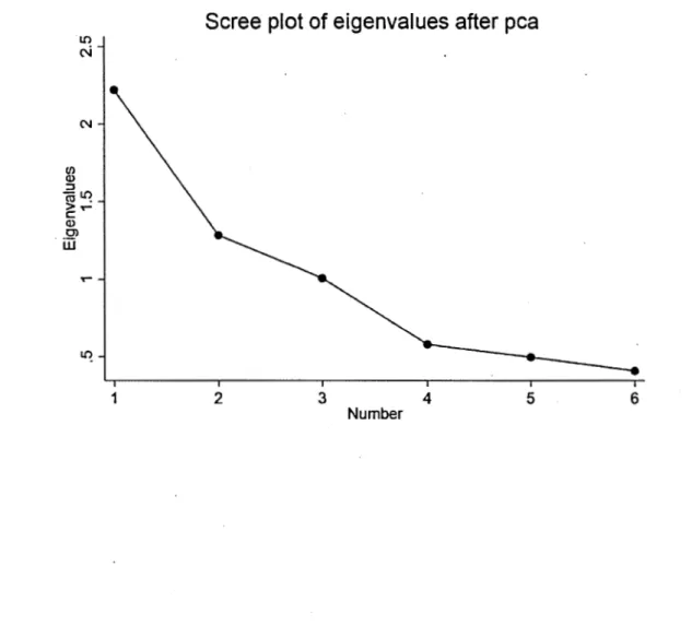
The aim was to generate aggregating weights for the composite score, although the PCA results also provide insights into correlations among the three CA dimensions. Only the components with an eigenvalue greater than 1 were retained, in accordance with the Kaiser's criterion (see Figure 2). The idea of this criterion is that the amount of variation explained by a factor is represented by the 'eigenvalues; an eigenvalue of 1 represents a substantial amount of variation (Field, 2009, p. 640). Furthermore, according to Field (2009), even if Kaiser's criterion tends to overestimate the number of factors to retain, there is some evidence that it is accurate when there are less than 30 variables, which is the case in our research.
Figure 2. Scree plot of the eigenvalues after the principal component analysis
lO C\Î N :::s -1!> ~r= C: Q) C) iii
...
1Scree plot of eigenvalues after pca
2 3 4 5 6