HAL Id: tel-02173705
https://pastel.archives-ouvertes.fr/tel-02173705
Submitted on 4 Jul 2019HAL is a multi-disciplinary open access archive for the deposit and dissemination of sci-entific research documents, whether they are pub-lished or not. The documents may come from teaching and research institutions in France or abroad, or from public or private research centers.
L’archive ouverte pluridisciplinaire HAL, est destinée au dépôt et à la diffusion de documents scientifiques de niveau recherche, publiés ou non, émanant des établissements d’enseignement et de recherche français ou étrangers, des laboratoires publics ou privés.
Numerical optimization using stochastic evolutionary
algorithms : application to seismic tomography inverse
problems
Keurfon Luu
To cite this version:
Keurfon Luu. Numerical optimization using stochastic evolutionary algorithms : application to seismic tomography inverse problems. Geophysics [physics.geo-ph]. Université Paris sciences et lettres, 2018. English. �NNT : 2018PSLEM077�. �tel-02173705�
Numerical optimization using stochastic evolutionary
algorithms: application to seismic tomography inverse
problems
Optimisation numérique stochastique évolutionniste :
application aux problèmes inverses de tomographie
sismique
Soutenue parKeurfon LUU
Le 28 septembre 2018 École doctorale no398Géosciences,
Ressources Naturelles et
Environnement
SpécialitéGéosciences et
Géoingénierie
Composition du jury : M. CAUMON GuillaumeProfesseur, Université de Lorraine Rapporteur
M. TARITS Pascal
Professeur, Université de Bretagne Occidentale Rapporteur
M. BODET Ludovic
Maître de conférences, Sorbonne Université Examinateur
Mme GÉLIS Céline
Ingénieur de recherche, IRSN Examinatrice
Mme GESRET Alexandrine
Chargée de recherche, MINES ParisTech Examinatrice
M. NOBLE Mark
Maître de recherche, MINES ParisTech Examinateur
M. ROUX Pierre-François
Acknowledgements
Tout d’abord, je tiens à remercier mes jambes pour m’avoir supporté tout au long de mon parcours, mes bras pour toujours avoir été à mes côtés, sans oublier mes doigts sur lesquels j’ai toujours pu compter.
Plus sérieusement, je dois mes premiers remerciements à Mark Noble, mon directeur de thèse, qui m’a permis de travailler sur ce sujet tout en me laissant suffisamment de liberté pour me l’approprier (il me semble que le sujet initial portait sur la localisation. . . ). Je remercie également ma co-encadrante Alexandrine Gesret pour tout le temps qu’elle m’a accordé et ses précieux conseils durant la rédaction de ce manuscrit.
Je souhaiterais exprimer ma gratitude envers Guillaume Caumon et Pascal Tarits qui ont accepté d’être rapporteurs de ce travail (et de lire ce manuscrit pendant leurs vacances d’été), ainsi que Céline Gélis et Ludovic Bodet pour avoir accepté de faire partie de mon jury de thèse.
Mes sincères remerciements vont aussi à Philippe Thierry qui, en dépit de son agenda de ministre, a trouvé du temps pour m’aider et me conseiller sur le calcul haute performance, et qui m’a notamment permis de faire la rencontre de Skylake quand Katrina m’a laissé tomber (je parle d’ordinateurs hein, pas taper).
Mention spéciale à tous les autres membres du Labo de Géophy : Hervé, Pierre, Véronique, les deux gars de Magnitude Nidhal et Pierre-François, Maxime, Charles-Antoine, Yves-Marie, Jihane, Sven, Emmanuel, Yubing, Alexandre, Hao, Julien, Michelle, Tianyou, Ahmed et en passant par le Brésil, Tiago. Merci pour votre bonne humeur et toutes les discussions que l’on a pu avoir pendant les (trop) nombreuses pauses café.
Que seraient ces remerciements si j’oubliais tous les membres de ma famille (de près ou de loin généalogiquement ou géographiquement) qui m’ont connu et soutenu depuis mes premières lignes de commande (sous DOS pour lancer des jeux, bien entendu). En particulier, je dois beaucoup à baba mama qui ont fait beaucoup de sacrifices pour ma soeur, mon frère et moi, et qui, malgré leurs modestes moyens, nous ont toujours encouragés et poussés à donner le meilleur de nous.
Enfin, je voudrais dédier ce mémoire à ma femme An qui, plus que toutes les parties de mon corps susmentionnées, n’a jamais cessé de me supporter (dans les deux sens du terme), d’être à mes côtés et de m’encourager durant ces trois longues années. Xiexie ni wo de baobei.
ii
Résumé
La tomographie sismique des temps de trajet est un problème d’optimisation mal-posé du fait de la non-linéarité entre les temps et le modèle de vitesse. Par ailleurs, l’unicité de la solution n’est pas garantie car les données peuvent être expliquées par de nombreux mod-èles. Les méthodes de Monte-Carlo par Chaînes de Markov qui échantillonnent l’espace des paramètres sont généralement appréciées pour répondre à cette problématique. Cependant, ces approches ne peuvent pleinement tirer parti des ressources computationnelles fournies par les super-calculateurs modernes. Dans cette thèse, je me propose de résoudre le prob-lème de tomographie sismique à l’aide d’algorithmes évolutionnistes. Ce sont des méthodes d’optimisation stochastiques inspirées de l’évolution naturelle des espèces. Elles opèrent sur une population de modèles représentés par un ensemble d’individus qui évoluent suivant des processus stochastiques caractéristiques de l’évolution naturelle. Dès lors, la population de mod-èles peut être intrinsèquement évaluée en parallèle ce qui rend ces algorithmes particulièrement adaptés aux architectures des super-calculateurs. Je m’intéresse plus précisément aux trois algorithmes évolutionnistes les plus populaires, à savoir l’évolution différentielle, l’optimisation par essaim particulaire, et la stratégie d’évolution par adaptation de la matrice de covariance. Leur faisabilité est étudiée sur deux jeux de données différents: un jeu réel acquis dans le contexte de la fracturation hydraulique et un jeu synthétique de réfraction généré à partir du modèle de vitesse Marmousi réputé pour sa géologie structurale complexe.
Mots Clés: algorithme évolutionniste, tomographie sismique, problème inverse, calcul haute performance, intelligence artificielle
iv
Abstract
Seismic traveltime tomography is an ill-posed optimization problem due to the non-linear relation-ship between traveltime and velocity model. Besides, the solution is not unique as many models are able to explain the observed data. The non-linearity and non-uniqueness issues are typically addressed by using methods relying on Monte Carlo Markov Chain that thoroughly sample the model parameter space. However, these approaches cannot fully handle the computer resources provided by modern supercomputers. In this thesis, I propose to solve seismic travel-time tomography problems using evolutionary algorithms which are population-based stochastic optimization methods inspired by the natural evolution of species. They operate on concurrent individuals within a population that represent independent models, and evolve through stochastic processes characterizing the different mechanisms involved in natural evolution. Therefore, the models within a population can be intrinsically evaluated in parallel which makes evolutionary algorithms particularly adapted to the parallel architecture of supercomputers. More specifically, the works presented in this manuscript emphasize on the three most popular evolutionary algorithms, namely Differential Evolution, Particle Swarm Optimization and Covariance Matrix Adaptation - Evolution Strategy. The feasibility of evolutionary algorithms to solve seismic tomography problems is assessed using two different data sets: a real data set acquired in the context of hydraulic fracturing and a synthetic refraction data set generated using the Marmousi velocity model that presents a complex geology structure.
Keywords: evolutionary algorithm, seismic tomography, inverse problem, high performance computing, artificial intelligence
Contents
1 Introduction 1
1.1 General context . . . 1
1.2 Inverse problems in geophysics . . . 2
1.3 Overview . . . 5
1.4 Contributions . . . 7
2 Introduction to evolutionary algorithms 11 2.1 Black-box optimization . . . 12
2.1.1 Misfit function . . . 12
2.1.2 Derivative-free algorithms . . . 14
2.2 Evolutionary algorithms . . . 15
2.2.1 Differential Evolution . . . 17
2.2.2 Particle Swarm Optimization . . . 19
2.2.3 Covariance Matrix Adaptation - Evolution-Strategy . . . 23
2.3 Sample codes . . . 27
2.3.1 Differential Evolution . . . 27
2.3.2 Particle Swarm Optimization . . . 28
2.3.3 Covariance Matrix Adaptation - Evolution Strategy . . . 28
2.4 Parallel implementation . . . 30
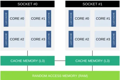
2.4.1 About supercomputers. . . 30
2.4.2 Hybrid parallel programming . . . 32
2.5 Conclusion . . . 34
3 1D traveltime tomography 35 Abstract . . . 36
3.1 Introduction . . . 37
viii CONTENTS
3.2.1 Particle Swarm Optimization . . . 38
3.2.2 Premature convergence . . . 39
3.2.3 Competitive Particle Swarm Optimization . . . 40
3.3 Robustness testing . . . 44 3.3.1 Sensitivity analysis . . . 44 3.3.2 Benchmark . . . 46 3.3.3 Importance sampling. . . 46 3.4 Numerical example . . . 47 3.4.1 Acquisition . . . 47 3.4.2 Inversion results . . . 49
3.5 Hybrid parallel implementation . . . 53
3.6 Discussion and conclusion . . . 54
3.7 Appendice. . . 55
3.7.1 PSO algorithm . . . 55
3.7.2 CPSO algorithm . . . 56
3.7.3 Benchmark test functions . . . 57
3.7.4 Sensitivity analysis . . . 57
4 Refraction traveltime tomography 59 Abstract . . . 60
4.1 Introduction . . . 60
4.2 Theory and method . . . 62
4.2.1 Evolutionary algorithms . . . 63
4.2.2 Control parameter values . . . 67
4.3 Numerical example . . . 67
4.3.1 Synthetic data and parametrization . . . 67
4.3.2 Weighted mean model and standard deviation . . . 68
4.3.3 Initial models . . . 70
4.3.4 Results . . . 72
4.3.5 Scalability . . . 77
4.4 Discussion and conclusion . . . 78
5 Neural network automated phase onset picking 81
Abstract . . . 82
5.1 Introduction . . . 83
5.2 Description . . . 84
5.2.1 Artificial neural network . . . 84
5.2.2 Attributes . . . 85
5.3 Methodology . . . 88
5.3.1 Real data set . . . 88
5.3.2 Attributes selection . . . 90
5.3.3 Training . . . 93
5.3.4 Skewing the training set . . . 94
5.3.5 Prediction . . . 95
5.4 Conclusion . . . 97
6 Conclusions and perspectives 99 6.1 Conclusions. . . 100
6.1.1 1D traveltime tomography . . . 100
6.1.2 Refraction traveltime tomography . . . 101
6.1.3 Neural network automated phase onset picking . . . 101
6.2 Perspectives . . . 102
6.2.1 Improving parallelism and convergence: Island models. . . 102
6.2.2 Improving phase onset picking: Bayesian neural network and neuroevolution102 6.2.3 Use of velocity model uncertainties . . . 103
A Eikonal equation 105 B Surface wave tomography 109 B.1 Introduction . . . 110
B.2 Forward problem: Thomson-Haskell propagator . . . 110
B.2.1 Rayleigh wave in a layered medium . . . 110
B.2.2 Roots search . . . 114
B.3 Inversion . . . 114
x CONTENTS
C Propagation of velocity uncertainties to locations 117
Abstract . . . 118
C.1 Introduction . . . 118
C.2 From optimization to uncertainty quantification . . . 119
C.3 Propagation of velocity uncertainties to locations . . . 120
C.3.1 Inversion . . . 120
C.3.2 Acceptable models . . . 120
C.3.3 Velocity models clustering . . . 121
C.4 Conclusion . . . 123
Chapter 1
Introduction
Contents
1.1 General context . . . 1
1.2 Inverse problems in geophysics . . . 2
1.3 Overview . . . 5
1.4 Contributions . . . 7
1.1
General context
This thesis is supported by the GEOTREF project (www.geotref.com). This project is funded by ADEME in the frame of les Investissements d’Avenir program. Partners of the GEOTREF project are Kidova, Teranov, MINES ParisTech, ENS Paris, GeoAzur, GeoRessources, IMFT, IPGS, LHyGes, UA, and UCP-GEC. GEOTREF is a multi-disciplinary platform for innovation and demonstration activities for the exploration and development of high geothermal energy in fractured reservoirs.
The initial topic of this work aimed at characterizing the seismicity induced by the hydraulic fracturing process in the context of geothermal energy. In non-conventional hydrocarbon reservoirs or geothermal systems, fluid is usually injected into reservoirs to improve their permeability. This process can lead to the failure of the medium due to the changes of its physical properties (e.g. stress, pore pressure). Populated areas must be monitored in case of increasing seismic rate and/or magnitude. For instance, an earthquake of magnitude 3.4 has been caused by a geothermal project in Basel (Switzerland) in 2006 (Deichmann and Giardini (2009)).
Microseismic monitoring is currently the only method available to follow the state of the fracking and is thus required for security reasons. In the last decades, it has been a key tool to understand and delineate hydraulic fracture geometry (Sasaki (1998), Maxwell et al. (2002), Rothert and Shapiro (2003), Warpinski, Wolhart and Wright (2004), Calvez et al. (2007), Daniels et al.
2 1.2. INVERSE PROBLEMS IN GEOPHYSICS
(2007), Warpinski (2009), Maxwell et al. (2010)). It consists in locating microseismic events to constrain the geometry of the fractures. Event locations are strongly affected by the quality of the velocity model used and is usually disregarded in the interpretation (Cipolla et al. (2011)). Maxwell (2009) has shown on a simple synthetic model that an error on the velocity of only a few percent can produce a shift in an event location that can reach several hundreds of meters. In routine microseismic monitoring, a layered velocity model is constructed from acoustic logs that measure both compressional (P-) and shear (S-) wave velocities. The velocity model is then calibrated using perforation shots from known locations (Eisner et al. (2009)). Finally, the quality of the calibrated velocity model can be assessed by evaluating the errors in perforation shot locations.
In the frame of geothermal energy, microseismic events are typically recorded by a limited number of receivers deployed on the near-surface and can be used to image the reservoir. Such an acquisition geometry is not ideal as the ray paths from the perforation shots to the receivers do not correctly cover the medium traversed. Consequently, a given velocity model that gives small perforation shot location errors is only one of the many velocity models that can accurately relocate the shots. In addition, Gesret et al. (2015) showed that more reliable locations of hypocenters with their associated uncertainties can be obtained by propagating the velocity model uncertainties to the event locations. Therefore, an accurate velocity model must be derived and its uncertainties acknowledged to enable reliable interpretation of microseismic data.
Broadly speaking, velocity models are reconstructed through a tomographic procedure that iteratively tries to fit a model to match the observed data. This procedure is usually called an inversion as one wants to find the model that could have generated a given data set. In this manuscript, I particularly emphasize on first arrival traveltime tomography that aims at building the velocity model using the traveltimes observed from the seismic sources to all the receivers. The methodology initially developed to solve the tomographic problem in the context of microseismicity is applied to other tomographic problems that could potentially find an interest in geothermal reservoir characterization. First arrival traveltime tomography is an optimization problem and thus requires an accurate forward problem and an optimization algorithm for its resolution.
In this introduction, I first describe the principles of inverse problems. The limitations of the conventional methods used to solve an inverse problem in geophysics motivate the need to develop more computer efficient algorithms.
1.2
Inverse problems in geophysics
Solving an inverse problem consists in finding the physical model that explains the data by minimizing the misfit between the observed data and the data predicted by the model. Therefore, it is necessary to define the physical law that accurately describes the relation between the data and a physical model. In inversion, this operation is known as the foward modeling. Let d = {d1; :::; dN} be a discrete vector of N data points, m = {m1; :::; md} a physical model
described by d parameters, and g the forward modeling operator such that
d = g (m) : (1.1)
The quality of the data is strongly affected by the level of noise recorded during the measurements. In addition, mathematical models are oftenly subject to hypothesis and approximations and thus do not exactly reproduce the true physics. Therefore, an additional term ε that accounts for both
the errors in the data and the forward modeling must be considered and Equation (1.1) can be rewritten as
d = g (m) + ε: (1.2)
In first arrival traveltime tomography, d and m are the traveltime data and the velocity model, respectively. First arrival traveltimes can be accurately computed by solving the Eikonal equation that links the velocities of the propagation medium to the traveltimes under the high frequency approximation. This approximation is only valid when the signal wavelength is negligible with respect to the characteristic wavelength of the medium. A full and detailed presentation of the dynamic of acoustic waves can be found in Chapman (1985), Sheriff and Geldart (1995) and ˇCervený (2001) and is beyond the scope of this thesis. However, a short description of the underlying Eikonal equation is reviewed in AppendixA. The Eikonal equation is written
|∇T |2 = 1
c2 (1.3)
where |·| denotes the absolute value, ∇ the gradient operator, T the traveltime and c the velocity of the medium. It is a partial differential equation that can be solved either analytically for simple velocity models, or numerically by using ray-tracing (Julian and Gubbins (1977), ˇCervený (1987), Um and Thurber (1987)) or a finite-difference Eikonal solver (Vidale (1988), Vidale (1990), Podvin and Lecomte (1991), Trier and Symes (1991)). In this thesis, the finite-difference Eikonal solver proposed by Noble, Gesret and Belayouni (2014) is used to compute accurate traveltimes. Inverse problems rely on a scalar objective function that measures the misfit between the observed and the theoretical data to assess the quality of the model parameters, and is usually called misfit function. The optimal model corresponds to the model that yields the global minimum misfit function value. In other words, solving an inverse problem requires the minimization of the misfit function E under the constraint m ∈ Ω (feasible space) such that
∀m ∈ Ω; mopt = argmin (E (m)) : (1.4)
Although other norms can be found in the literature, the misfit function is usually defined in the least-squares sense in geophysics, following
E (m) = »“ dobs− g (m)”>“dobs − g (m)”– 1 2 (1.5) where dobs stands for the observed data.
Misfit functions encountered in geophysical inverse problems are ill-posed and highly multi-modal due to the non-linearity between the models and the data (Delprat-Jannaud and Lailly (1993), Zhang and Toksöz (1998)). The non-linearity of first arrival traveltime tomography problems are most oftenly addressed by using derivative-based (i.e. gradient) optimization methods (White (1989), Zelt and Barton (1998), Taillandier et al. (2009), Rawlinson, Pozgay and Fishwick (2010), Noble et al. (2010)) combined with a regularization procedure to make the problem better posed (Hansen and O’Leary (1993), Menke (2012), Tikhonov et al. (2013)). Derivative-based optimization methods are local optimization algorithms that iteratively update a model such that the misfit function value decreases over time, the direction of updates being given by the gradient of the misfit function with respect to the model parameters. Derivative-based algorithms include the steepest descent methods (Nemeth, Normark and Qin (1997), Taillandier et al. (2009)), the conjugate gradient methods (Luo and Schuster (1991), Zhou et al. (1995)), Gauss-Newton methods (Delbos et al. (2006)), Quasi-Newton methods (Liu and Nocedal (1989), Nash and Nocedal (1991)) and Newton methods (Gerhard Pratt, Shin and Hicks (1998)). Nowadays methods can efficiently compute the gradient of the misfit function by using the adjoint state method (Chavent (1974), Plessix (2006)).
4 1.2. INVERSE PROBLEMS IN GEOPHYSICS
As previously mentioned, one of the main challenges dealt when reconstructing a velocity model is the non-uniqueness of the solution. Besides the unconstraining geometry inherent to typical microseismic acquisition, additional sources of approximations and errors can contribute to the non-uniqueness of the velocity model such as the parametrization chosen and the theory behind the forward modeling (Tarantola (2005)). The adjoint state method applied to compute the gradient when using derivative-based algorithms does not provide the sensitivity of the solution to the errors and additional expensive calculations of the Fréchet derivatives are required (Plessix (2006)). Moreover, derivative-based algorithms are local optimization methods that make the assumption of a unique solution that presents a good trade-off between data fit and regularization and strongly depend on the initial solution (Menke (2012)). For highly non-linear problems such as traveltime tomography, these approaches are not suitable when it comes to uncertainty quantification.
From a theoretical point of view, global optimization methods that sample the model parameter space are required to appraise the uncertainties. Geophysicists usually resort to probabilistic approaches that rely on the Bayes theorem combined with Markov Chain Monte Carlo algorithms (MCMC, Tarantola and Valette (1982), Scales and Snieder (1997), Ulrych, Sacchi and Woodbury (2001), Scales and Tenorio (2001)). In the Bayesian framework, the model parameters are random variables distributed accordingly to a probability distribution. Interest of this approach is two-fold: one can use the a priori knowledge about the parameter values to better constrain the estimation of the model parameters (an uninformative prior distribution can be defined otherwise); it thoroughly samples the model space and provides reliable parameter uncertainty estimates which offers a way to tackle the non-linear and non-uniqueness issues. MCMC algorithms have been first introduced in geophysics by Keilis-Borok and Yanovskaya (1967) and have been widespreadly used for optimization and sampling purpose to solve various types of geophysical inverse problem since then. Press (1968), Wiggins (1969) and Press (1970) were the first to apply MCMC algorithms to fit Earth models to seismological data. Cary and Chapman (1988) and Koren et al. (1991) addressed the problem of seismic waveform fitting using MCMC methods. Zhang and Toksöz (1998) used an MCMC approach to estimate the uncertainties of a velocity model obtained by a derivative-based optimization method. Other than in seismic studies, they also found applications in magnetotelluric (Jones and Hutton (1979), Jones, Olafsdottir and Tiikkainen (1983), Grandis, Menvielle and Roussignol (1999)) and electrical (Schott et al. (1999), Malinverno and Torres-Verdín (2000), Ramirez et al. (2005)) studies. A comprehensive but non-exhaustive review of their applications in geophysics can be found in Mosegaard and Tarantola (1995) and Sambridge and Mosegaard (2002). Nonetheless, classical MCMC algorithms can become inefficient with increasing number of parameters and multi-modal distributions as they can be easily trapped in a local mode. Many algorithms based on MCMC have been proposed to address its shortcomings such as the well-known Simulated Annealing (SA, Kirkpatrick, Gelatt and Vecchi (1983)), reversible-jump Markov Chain Monte Carlo (rj-MCMC, Green (1995)) or by using simultaneous interactive Markov Chains (Romary (2010), Sambridge (2014), Bottero et al. (2016)). On the one hand, rj-MCMC provides an interesting way to solve inverse problems without the requirement to fix the number of unknowns to optimize a priori and has been first applied in geophysics by Malinverno and Leaney (2000). Such inversion algorithms are usually qualified as transdimensional since they jump between parameter subspaces of different dimensionality. Bodin and Sambridge (2009) applied this algorithm to the seismic tomography problem. More recently, Piana Agostinetti, Giacomuzzi and Malinverno (2015) solved a three-dimensional local earthquake tomography problem using a transdimensional approach. On the other hand, interactive Markov Chains methods tackle the sequential nature of MCMC algorithms by allowing the sampling to be done in parallel. However, these methods are not straightforward to implement and remain sensitive to their control parameter values which are not easy to tune.
Microseismic data are required to be processed in real-time which motivates the need to develop and implement computationally efficient algorithms. In this thesis, I essentially work with another class of global optimization algorithms that has been growing in popularity in the last decades and are known as evolutionary algorithms. These methods are stochastic optimization methods inspired by the natural evolution of species and simultaneously operate on a set of candidate solutions called a population. Evolutionary algorithms have been quite overlooked by the geophysical community mostly due to the computational cost as the misfit function requires to be evaluated numerous times. Only few applications are available in the geophysical literature. More specifically, they have been applied to solve magnetotelluric inverse problems (Shaw and Srivastava (2007), Grayver and Kuvshinov (2016), Xiong et al. (2018)), gravity inversion (Zhang et al. (2004), Toushmalani (2013), Pallero et al. (2015), Ekinci et al. (2016)), history matching for reservoir characterization (Schulze-Riegert et al. (2001), Hajizadeh, Christie and Demyanov (2010), Mohamed et al. (2010), Fernández Martínez et al. (2012)), earthquake location (Sambridge and Gallagher (1993), R˚užek and Kvasniˇcka (2001), Han and Wang (2009)), surface-wave inversion (Wilken and Rabbel (2012), Song et al. (2012), Poormirzaee (2016)), and traveltime tomography (Tronicke, Paasche and Böniger (2012), Rumpf and Tronicke (2015), Poormirzaee, Moghadam and Zarean (2015)). Nonetheless, with the rise in computational power mainly brought by the parallel architectures of supercomputers, evolutionary algorithms are becoming an interesting alternative to conventionally used optimization methods as they are intrinsically parallel. Originally, evolutionary algorithms have not been designed for uncertainty quantification. However, as stochastic algorithms, they can be run several times to explore and sample different subspaces of the model parameter space (Sen and Stoffa (1996)).
1.3
Overview
The manuscript is organized as followed:
• In Chapter2, I give an introduction to evolutionary algorithms in the framework of black-box optimization. First, I introduce the concepts of black-box optimization and evolutionary algorithms. Many evolutionary algorithms have been proposed in the literature. However, this thesis mainly emphasizes on the three most popular and efficient evolutionary algo-rithms, namely the Differential Evolution (DE), the Particle Swarm Optimization (PSO) and the Covariance Matrix Adaptation - Evolution Strategy (CMA-ES). These algorithms are thoroughly described in Chapter 2. For each method, I detail the algorithm and the underlying equations, and try to give a more intuitive explanation about how they work. A sample working code (written in Python) is also provided for the three methods. Finally, I give a brief description of the hybrid parallel programming paradigm used throughout this thesis to solve seismic tomography problems using evolutionary algorithms in reasonable computation time;
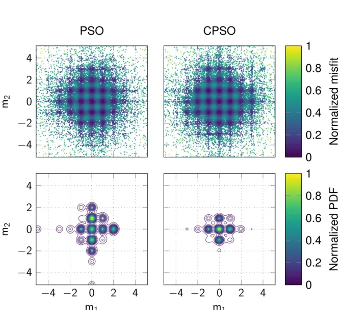
• In Chapter3, I principally focus on PSO for its efficiency and ease of implementation. I present a new optimization algorithm based on PSO that tackles its main shortcoming. I called this new algorithm Competitive Particle Swarm Optimization (CPSO). Indeed, PSO is particularly prone to stagnation and premature convergence (i.e. convergence toward a local minimum) like any evolutionary algorithm. Therefore, I suggest a simple yet efficient modification of the original implementation that improves the diversity of the swarm. I demonstrate on several benchmark test functions that CPSO is more robust in terms of convergence and sensitivity to its parameters compared to PSO. Besides, I show on a highly multi-modal function that CPSO can be used for rapid uncertainty quantification.
6 1.3. OVERVIEW
Estimation of the Probability Density Function is done by sampling the model parameter space through several independent inversions. The methodology is applied to a first arrival traveltime tomography problem using a real 3D microseismic data set acquired in the context of induced seismicity and is compared to a conventional MCMC sampler. The results demonstrate that CPSO is able to reach the stationary regime much faster and provides uncertainty estimates consistent with the ones obtained with the MCMC sampler. Finally, I analyze the scalability of CPSO for this tomographic problem by evaluating its parallel performance. Note that the results obtained in this work have been further used in AppendixC;
• Chapter 4aims at studying the feasibility of evolutionary algorithms to solve a problem of larger dimensionality (> 102). To this end, I extend the methodology introduced in
Chapter3to the highly non-linear and multi-modal problem of refraction tomography that could potentially find an interest in geothermal reservoir characterization. I apply the methodology on the Marmousi velocity model that presents a complex geological structure and compare the performances of DE, CPSO and CMA-ES. The synthetic traveltime data are generated considering a surface acquisition geometry that consists of two hundred shots and four hundred receivers which results in poor ray coverage in depths. The velocity model is parametrized using 2D cardinal B-splines. I investigate the influences of the initial velocity models, the population size and the maximum number of iterations. Evolutionary algorithm are stochastic optimization methods and should ideally be insensitive to the initial population. However, I show that using a realistic initial population instead of fully random models can significantly improves the convergence of these algorithms on the refraction tomography problem. Finally, I assess the benefits and shortcomings of each algorithm by performing scalability and statistical analysis over the results obtained after several runs;
• Microseismic monitoring requires an efficient automated phase onset picking algorithm for real-time microseismic event locations induced by hydraulic fracturing (Calvez et al. (2007)). To a lesser extent, errors in arrival times can also contribute to errors in locations. Common automated phase onset pickers are not designed to estimate arrival time uncertainties. In Chapter5, I describe an automated phase onset picking algorithm based on a multi-attributes neural network. It is noteworthy that this chapter is the result of a project in collaboration with ENS Paris and ENSG, the main emphasis of this thesis remains the application of evolutionary algorithms to seismic tomography. Principles of neural networks are merely described and only important notions required to the understanding of the chapter are introduced. The chapter is written as a description of a computer software implemented in Python. I describe the methodology by applying the workflow on a real data set acquired at the laboratory scale. Optimal attributes and their parameters are selected thanks to a scatter-plot matrix. Then, a neural network can be trained using either a derivative-based optimizer or an evolutionary algorithm. The probability map output by the neural network model is used to predict a phase onset, assess its error or reject a false positive. Finally, the picker model is applied to the whole data set to predict the arrival times and relocate the microseismic events. The results obtained are promising in terms of accuracy and quantification of arrival time picking errors;
• In Chapter6, I summarize the main conclusions drawn throughout this manuscript. I also propose several prospects of improvement, such as the island models to enhance the performance of evolutionary algorithms, using neuroevolution to find the optimal neural network architecture, and what to do with velocity model uncertainties once quantified;
• In AppendixA, I detail the derivation of the elasto-dynamic equation to obtain the Eikonal equation underlying the main forward modeling involved in this thesis (i.e. computation of first arrival traveltimes);
• In Appendix B, I apply the same methodology as described in Chapter 3 to a surface wave tomography problem. The forward modeling is first briefly detailed and consists in estimating the frequency-dependent modal dispersion curves using the Thomson-Haskell propagator method. Finally, I show an application to a real data set that consists of three dispersion curves obtained by the joint use of ambient noise correlation and Multiple signal characterization algorithm (MUSIC);
• Gesret et al. (2015) has shown that accurate hypocenter locations with more reliable uncertainties can be retrieved by accounting for the velocity model uncertainties during the location procedure. This is achieved by locating the events in all the velocity models sampled which can be computationally inefficient. In Appendix C, I propose to use an unsupervised learning algorithm (Mini-batch K-Means) to find a subset of velocity models for the location. The methodology is applied to the velocity models sampled in Chapter3.
1.4
Contributions
As my work mainly focuses on computation time performance, I first cleaned and optimized the existing finite-difference Eikonal solver proposed in Noble, Gesret and Belayouni (2014). I added several functions for parallel traveltime grid computation using OpenMP and a posteriori ray-tracing based on the work of Podvin and Lecomte (1991). The code is originally written in Fortran and has been wrapped into a Python package for faster prototyping. I also implemented different evolutionary algorithms such as DE, PSO and CMA-ES, and developed CPSO, a new evolutionary algorithm based on PSO that improves its robustness. All the evolutionary algorithms are parallelized using MPI. The codes are available on my GitHub page as Python packages or Fortran modules:
• FTeikPy: object-oriented module that computes accurate first arrival traveltimes in 2D and 3D heterogeneous isotropic velocity model. Available atgithub.com/keurfonluu/FTeikPy;
• Forlab: Fortran library I wrote that contains more that one hundred polymorphic basic functions inspired by Matlab and NumPy. All the Fortran softwares I wrote have core dependency to this library. Available atgithub.com/keurfonluu/Forlab;
• StochOPy: user-friendly routines to sample or optimize objective functions with the most popular evolutionary algorithms, as described in Chapter2. For completeness and out of curiosity, MCMC sampling algorithms such as Metropolis-Hastings and Hamiltonian Monte Carlo have been implemented in this package. A Graphical User Interface (GUI) is available to test the different algorithms and their parameters on several benchmark test functions. Available atgithub.com/keurfonluu/StochOPy;
• StochOptim: same as StochOPy (without GUI) but in Fortran. This module has been used in Chapter 3 and Chapter 4 to solve the tomographic problems. Available at github.com/keurfonluu/StochOptim.
8 1.4. CONTRIBUTIONS
During my thesis, I also worked with other students on other inverse problems. In the frame of the GEOTREF project, I collaborated with the Laboratoire de Géologie at the ENS Paris and ENSG to study the geomechanical properties of an andesite sample from la Guadeloupe. My work consisted in relocating the acoustic emissions recorded using a conventional tri-axial cell. Therefore, I implemented an automated neural network phase onset picker to pick the arrival times for event relocations. In addition, I worked with a colleague on dispersion curve inversion in the context of ambient noise surface wave tomography. I implemented the forward modeling in Fortran and wrapped it into a Python module, the dispersion curves are inverted using StochOPy. The computer codes used for the two collaborations have also been made available on GitHub: • AIPycker: pythonic object-oriented module for automated phase onset picking using a
multi-attributes neural network, as described in Chapter5. It depends on NumPy, SciPy, ObsPy, Pandas, Matplotlib, Scikit-learn and StochOPy. It includes a GUI for manual onset picking and neural network training through a wizard. The package is in early development and the methodology still has to be improved. However, AIPycker is more user-friendly and has shown superior results compared to the commercial software used at ENS Paris. Available atgithub.com/keurfonluu/AIPycker;
• EvoDCinv: surface wave dispersion curve inversion using evolutionary algorithms. The package can handle inversion of multi-modal dispersion curves and both Rayleigh and Love waves, as described in AppendixB. Available atgithub.com/keurfonluu/EvoDCinv. The results obtained presented in this manuscript have been subject to oral presentations in two international conferences, and submitted for publication:
• Zhi Li, Keurfon Luu, Aurélien Nicolas, Jérôme Fortin and Yves Guéguen, 2016. “Fluid-induced rupture on heat-treated andesite.” 4th International Workshop on Rock Physics; • Keurfon Luu, Mark Noble, Alexandrine Gesret, 2016. “A competitive particle swarm
optimization for nonlinear first arrival traveltime tomography.” 2016 SEG International Expo-sition and Annual Meeting. Society of Exploration Geophysicists. doi: 10.1190/segam2016-13840267.1;
• François Bonneau, Keurfon Luu, Aurélien Nicolas and Zhi Li, 2017. “Toward an under-standing of the relationship between fracturing process and microseismic activity: study at the laboratory scale.” 2017 RING Meeting;
• Keurfon Luu, Mark Noble, Alexandrine Gesret, Nidhal Belayouni and Pierre-François Roux, 2017. “Propagation of velocity uncertainties to Microseismic locations using a competitive Particle Swarm Optimizer.” 79th EAGE Conference and Exhibition 2017; • Keurfon Luu, Mark Noble, Alexandrine Gesret, Nidhal Belayouni and Pierre-François
Roux, 2018. “A parallel competitive Particle Swarm Optimization for non-linear first arrival traveltime tomography and uncertainty quantification.” Computers and Geosciences 113 (August 2017). Elsevier Ltd: 81–93. doi:10.1016/j.cageo.2018.01.016;
• Marc Peruzzetto, Alexandre Kazantsev, Keurfon Luu, Jean-Philippe Métaxian, Frédéric Huguet and Hervé Chauris, 2018. “Broadband ambient noise characterization by joint use of cross-correlation and MUSIC algorithm.” Geophysical Journal International 215(2): 760-779 (November 2018). doi:10.1093/gji/ggy311;
• Keurfon Luu, Mark Noble, Alexandrine Gesret and Philippe Thierry, 2018. “Toward large scale stochastic refraction tomography: a comparison of three evolutionary algorithms.” Geophysical Prospecting. Under review.
Chapter 2
Introduction to evolutionary
algorithms
Contents
2.1 Black-box optimization . . . 12 2.1.1 Misfit function . . . 12 2.1.2 Derivative-free algorithms . . . 14 2.2 Evolutionary algorithms . . . 15 2.2.1 Differential Evolution . . . 17 2.2.2 Particle Swarm Optimization . . . 19 2.2.3 Covariance Matrix Adaptation - Evolution-Strategy . . . 23 2.3 Sample codes . . . 27 2.3.1 Differential Evolution . . . 27 2.3.2 Particle Swarm Optimization . . . 28 2.3.3 Covariance Matrix Adaptation - Evolution Strategy . . . 28 2.4 Parallel implementation . . . 30 2.4.1 About supercomputers. . . 30 2.4.2 Hybrid parallel programming . . . 32 2.5 Conclusion . . . 34Ce chapitre est une introduction aux algorithmes évolutionnistes dans le contexte de l’optimisation dite boîte-noire. Ces algorithmes sont des méthodes stochastiques opérant sur une population de modèles représentés par des individus, et réputés pour être plus robustes que les approches
12 2.1. BLACK-BOX OPTIMIZATION
basées sur les méthodes de Monte-Carlo en termes d’optimisation. Les algorithmes évolu-tionnistes sont notamment très adaptés au calcul sur architecture parallèle, ce qui leur permet de mieux tirer partie des ressources computationnelles offertes par les super-calculateurs modernes par rapport aux méthodes de Monte-Carlo. J’introduis en premier lieu le concept d’optimisation boîte-noire avant de parler des algorithmes évolutionnistes. Bien que de nom-breux algorithmes évolutionnistes aient été proposés dans la littérature, je ne m’intéresserai qu’aux trois algorithmes les plus efficaces et populaires, à savoir l’évolution différentielle (Dif-ferential Evolution, DE), l’optimisation par essaim particulaire (Particle Swarm Optimization, PSO), et la stratégie d’évolution par adaptation de la matrice de covariance (Covariance Matrix Adaptation - Evolution Strategy, CMA-ES). Pour chaque méthode, je détaille l’algorithme ainsi que les équations sous-jacentes, et j’essaie de donner une explication plus intuitive de leur fonctionnement. Je fournis notamment un exemple de code (écrit en Python) pour chacun des algorithmes. Enfin, j’introduis le parallélisme hybride adopté dans cette thèse pour la résolution des problèmes de tomographie sismique par des algorithmes évolutionnistes avec des temps de calcul raisonnables.
La PSO est plus amplement étudiée dans le Chapitre 3 avec une application sur un jeu de données microsismiques réel. J’y propose un nouvel algorithme que j’ai appelé la PSO Compétitive (CPSO) basé sur la PSO qui résout son principal défaut à savoir la convergence prématurée. La même méthodologie est notamment appliquée à un problème de tomographie des ondes de surface en AnnexeBoù seuls le problème direct et les données diffèrent. J’étends ensuite l’étude à un problème de tomographie des ondes réfractées dans le Chapitre4dont le but est d’analyser la faisabilité des algorithmes évolutionnistes pour la résolution d’un problème à grand nombre de paramètres en comparant les trois algorithmes évolutionnistes (DE, CPSO, CMA-ES) introduits dans ce chapitre.
Tous les algorithmes décrits dans ce chapitre sont disponibles en libre accès sur ma page GitHub :
• StochOPy : routines faciles à utiliser pour échantillonner ou optimiser une fonction d’objectif à l’aide des algorithmes évolutionnistes les plus populaires. Certains algo-rithmes d’échantillonnage MCMC sont aussi disponibles tels que l’algorithme de Metropolis-Hastings et le Monte-Carlo Hamiltonien. Une interface utilisateur graphique a notamment été implémentée pour tester les différents algorithmes ainsi que leurs paramètres sur de nombreuses fonctions de test. Disponible à l’adressegithub.com/keurfonluu/StochOPy; • StochOptim : même chose que StochOPy (sans interface graphique utilisateur) mais écrit
en Fortran. Ce module a été utilisé dans le Chapitre3et Chapitre4pour l’inversion des deux problèmes de tomographie. Disponible à l’adressegithub.com/keurfonluu/StochOptim.
2.1
Black-box optimization
2.1.1 Misfit function
An optimization problem consists in minimizing an objective function (or cost function) f (x): min
x∈Ωf (x) (2.1)
where Ω ⊂ Rd is the search space (or feasible space), d denoting the dimension of the problem.
V = 2000 m/s 0 20 40 60 80 100 0 20 40 60 X (m) Depth (m) 1000 1500 2000 2500 3000 0 0:2 0:4 0:6 0:8 1 Velocity (m/s) Nor maliz ed misfit
Figure 2.1: (Left) Synthetic earth model. The source and the receiver are respectively represented by the white disk and white triangle. (Right) Misfit function for different values of velocity (V ∈ [1000; 3000] m/s). The global minimum of the misfit function (at 2000 m/s) indicates the true velocity of the earth model.
function value f (x). In geophysics, the objective function measures the misfit between the observed data (e.g. traveltimes) and the data generated by a physical model (e.g. velocity model), and is thus usually referred to as the misfit function.
For instance, let us consider a simple traveltime tomography problem as depicted in Figure2.1 (left). The earth model is characterized by a homogeneous velocity model of V = 2000 m/s. A signal is emitted by a source point and recorded by a single receiver at a time T . In traveltime tomography, the inputs (e.g. data) are the traveltime T and the positions of the source point and receiver, and the unknown is the velocity V . The physical relationship that links the traveltime to the velocity is written
T (V ) = D
V (2.2)
where D denotes the distance between the source point and the receiver. The misfit function E is usually defined in the least-square sense following
E (V ) =|T − T (V )|2: (2.3)
Figure 2.1 (right) shows the misfit function landscape built by systematically evaluating the function for different velocity values. The global minimum indicates the true velocity of the earth model.
Note that the problem illustrated in Figure2.1is unidimensional and well-posed, and presents a convex misfit function with a trivial solution. The velocity can be found by a simple grid (i.e. exhaustive) search over a range of feasible velocities. This kind of search procedure can only be achieved when dealing with few variables to optimize and is inefficient in higher dimensions (> 5). Several other properties of a misfit function can make it difficult to solve, such as
• multi-modality: the misfit function presents several local minima that can easily trap a local optimization method, as shown in Figure2.2(left);
• non-separability: a function is said to be separable if each variable xi can be minimized independently of the values of the other variables, a separable function can thus be minimized by d one-dimensional optimizations, as shown in Figure2.2(middle);
• ill-conditioning: the condition number is the ratio of the largest to the smallest eigenvalues of the Hessian. A problem is said to be ill-conditioned if its condition number is large
14 2.1. BLACK-BOX OPTIMIZATION
Multi-modal Non-separable Ill-conditioned
Figure 2.2:(Left) Multi-modal function with four local minima. (Middle) Non-separable function represented by a rotated ellipsoid. (Right) Ill-conditioned function with one undetermined parameter.
(typically > 105). Ill-conditioning results in variables that exhibit significant discrepancies
in the sensitivity to their contributions to the misfit function value, as shown in Figure2.2 (right).
Real-world optimization problems are generally ill-posed, multi-modal, non-separable and often ill-conditioned, and require advanced optimization algorithms to be solved. In the following and for consistency with the remainder of the manuscript, the misfit function is denoted by E and the variables to optimize are referred to as model parameters consequently denoted by m.
2.1.2 Derivative-free algorithms
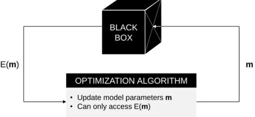
In the context of black-box optimization, no assumption is made on the misfit function such as whether it is continuous and/or differentiable. Black-box optimization algorithms can only query the misfit function values E (m) of any search point m of the feasible space Ω (i.e. zero order information). Thus, the algorithms do not have access to higher order information such as the gradient of the misfit function. However, it is still possible to approximate the gradient by finite-difference in the case where the misfit function is computationally cheap (i.e. fast to compute), and derivative-based optimization algorithms can thus be used in the black-box scenario. Real-world optimization problems deal with computationally expensive misfit functions (especially in geophysics) and numerical approximation of the gradient is not feasible in practice. Methods taylored for black-box optimization are the derivative-free optimization algorithms. These algorithms are called zero order methods as they only exploit the first term of the Taylor
BLACK BOX
• Update model parametersm
• Can only access E(m)
OPTIMIZATION ALGORITHM
m
E(m)
expansion of the misfit function (analogously, derivative-based methods are first or second order methods). While derivative-based methods are strictly deterministic in the sense that the solution is fully determined by the parameters and initial conditions, derivative-free methods can either be deterministic or stochastic (i.e. randomized). Deterministic derivative-free algorithms iteratively evaluate a set of points around the current point, and save the one that yields a lower misfit function value than the current point. It includes Simplex or Nelder-Mead’s method (Nelder and Mead (1965), McKinnon (1998)), pattern search (Hooke and Jeeves (1961), Torczon (1997)) or Powell’s method (Fletcher and Powell (1963), Powell (1964)). However, similarly to derivative-based methods, these algorithms are local optimization methods that depend on the initial conditions. On the other hand, evolutionary algorithms are stochastic derivative-free algorithms inspired by the natural evolution of species. This thesis mainly focuses on this type of black-box optimization algorithm.
2.2
Evolutionary algorithms
As many more individuals of each species are born than can possibly survive; and as, consequently, there is a frequently recurring struggle for existence, it follows that any being, if it vary however slightly in any manner profitable to itself, under the complex and sometimes varying conditions of life, will have a better chance of surviving, and thus be naturally selected. From the strong principle of inheritance, any selected variety will tend to propagate its new and modified form.
— Charles Darwin, On the Origin of Species (1859)
Natural evolution of species has been first theorized by Charles Darwin in his book On the Origin of Species published in 1859. He states that all the species have evolved from a common ancestor as a result of a process he called natural selection. According to Darwin’s theory of evolution, natural selection operates following “one general law leading to the advancement of all organic beings, namely, multiply, vary, let the strongest live and the weakest die”. Although his theory has been well received by other scientists, it has also raised several criticisms. The main criticism concerned the blending inheritance principle that would alter any beneficial characteristics and thus eliminate them after several generations. Blending inheritance has been discarded later in favor of the Mendelian inheritance discovered by Gregor Mendel in 1865 and presented in Experiments on Plant Hybridization (Mendel (1866), Hewlett and Mendel (1966)). Following the Mendelian inheritance principle, characteristics from parents are discretely passed to the offspring with a certain probability instead of being averaged. Modern population genetics is based on the combination of the principles brought by Darwin’s theory of evolution and Mendel’s principles of inheritance. All in all, evolution of populations is driven by three main mechanisms:
• Mutation: alteration of the characteristics of each individual within a population,
• Recombination: production of offspring with characteristic combinations that differ from those of either parent,
• Selection: pick offspring with characteristics that are beneficial and dispose of disadvanta-geous ones.
16 2.2. EVOLUTIONARY ALGORITHMS
Evolutionary algorithms are stochastic derivative-free optimization algorithms inspired by the natural evolution of species. The intrinsic operations are based on the genetic inheritance principle and the natural selection mechanism proposed respectively by Gregor Mendel and Charles Darwin. Broadly speaking, evolutionary algorithm consequently refers to all the optimiza-tion methods that operate on a concurrent populaoptimiza-tion of individuals (i.e. models) and generate new populations through genetic operations (mutation, recombination, selection). Evolutionary algorithms include Genetic algorithm (Holland (1973), Davis (1991)), Genetic programming (Koza (1992), Koza (1994)), Evolutionary programming (Fogel (1993), Fogel (1999)), Evolution strategies (Rechenberg (1973), Schwefel (1984)) and Swarm intelligence (Bishop (1989), Dorigo, Maniezzo and Colorni (1996)). Strictly speaking, Swarm intelligence is not a class of evolu-tionary algorithm as these methods are rather inspired by the social group behavior of certain species. However, they still fall into the broad definition of evolutionary algorithm and are usually considered as such. Likewise, the well-known Neighborhood algorithm (Sambridge (1999)) – at least among the geophysical community – can also be considered as an evolutionary algorithm. From an optimization point of view, evolution starts by selecting the fittest individuals in a population for reproduction to form the next generation. The chances of survival of the produced offspring depend on the quality of the characteristics they inherited from their parents. This process is iterated until a population with the fittest individuals is found. An evolutionary algorithm can be described by the following general template:
1. Given a parametrized distribution P (m|θ), initialize θ0,
2. For generation k = 1; 2; ::::
a. Sample n new candidates from distribution P “
m|θk−1”
→ m1; :::; mn,
b. Evaluate the candidates on E: E (m1) ; :::; E (mn),
c. Update parameters θk,
in which sampling (2a.) is the mutation and recombination mechanisms that create new indi-viduals, selection of individuals (2b.) evaluates the fitness of a new individual by assigning a scalar misfit value, and parameters update (2c.) corresponds to the remainder of the random phenomena that contribute to the genetic drift.
These simple mechanisms provide evolutionary algorithms interesting properties for optimiza-tion. They have demonstrated great flexibility and adaptability to solve a given task, robust performance and global search capabilities (Back, Hammel and Schwefel (1997)). Besides, evolutionary algorithms seem to be particularly suitable to solve multi-objective optimization problems as they are able to capture several Pareto-optimal solutions in a single run (Fonseca and Fleming (1995), Fonseca and Fleming (1998), Zitzler (1999), Deb (2001)). Evolutionary algo-rithms are also closely related to neuroevolution – a subfield of research in Artificial Intelligence – that consists in mutating and selecting the best neural networks to solve simple tasks (Ronald and Schoenauer (1994), Angeline, Saunders and Pollack (1994), Stanley and Miikkulainen (2002), Kassahun and Sommer (2005)). More recently, evolutionary algorithms have been successfully applied to train deep neural networks, a task usually reserved to derivative-based algorithms due to its high computational cost (Such et al. (2017), Conti et al. (2017), Lehman et al. (2017)). This has been made possible by exploiting the intrinsic parallel property of evolutionary algorithms that enables a better handling of all the computational power provided by modern supercomputers. This property can also find practical applications in geophysical inverse problems which is the main emphase of this thesis.
In the last decades, many new nature-inspired algorithms have been proposed such as Bees Algorithm (Pham et al. (2006)), Glowworm Swarm Optimization (Krishnanand and Ghose
(2006)), Cuckoo Search (Yang and Deb (2009)), Bat Algorithm (Yang (2010)), Flower Pollination Algorithm (Yang (2012)) or Grey Wolf Optimization (Mirjalili, Mirjalili and Lewis (2014)). This has attracted criticism among the research community whose main concern is the lack of novelty hidden behind a metaphor and argues that researchers should rather emphasize their works on analyzing existing algorithms (Sörensen (2015)). For instance, Weyland (2010) has shown that Harmony Search (Zong Woo Geem, Joong Hoon Kim and Loganathan (2001)) – an algorithm mimicking the improvisation of musicians – is simply a special case of (— + 1)-ES (Rechenberg (1973)) introduced about 30 years earlier. In a recent paper, Saka, Hasançebi and Geem (2016) performed a thorougher analysis of both methods, and concluded that the two algorithms are substancially different conceptually and operationally. Discussing who is right or wrong, whether one should stop proposing new nature-inspired algorithms or not, is beyond the scope of this thesis. This chapter only introduces the three most popular evolutionary algorithms, namely Differential Evolution (DE), Particle Swarm Optimization (PSO) and Covariance Matrix Adaptation - Evolution Strategy (CMA-ES). In the following, if not explicitly stated, the size of the population is denoted by n, the dimension of the problem by d and the iteration number (i.e. generation) by k.
2.2.1 Differential Evolution
Differential Evolution (DE) is a genetic programming algorithm introduced by Price (1996) and Storn and Price (1997). DE begins with a set of individuals called a population where each individual is a model solution to the problem to optimize. The population is initially sampled according to a uniform distribution. It differs from the well-known Genetic algorithm by its mutation and crossover (i.e. recombination) mechanisms.
Mutation
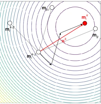
Unlike Evolution strategies, DE does not sample candidate solutions using predetermined probability distribution functions. DE perturbs a random existing population vector by adding to it the weighted difference between two different random population vectors. This mutation process is repeated for each individual in the population. For each target vector mk
i, DE generates a mutant vector vk i following vk i = mk−r1 1+ F “ mk−1 r2 − m k−1 r3 ” (2.4) where r1; r2; r3 ∈ {1; 2; :::; n} are three distinct random indices different from i, F ∈ [0; 2] is the mutation factor that weighs the differential variation“
mk−1 r2 − m k−1 r3 ” . Mutation is an important process that maintains diversity within the population and prevents premature convergence. Large mutation factor increases the search radius (i.e. diversity) at the expense of speed of convergence. The mutation mechanism is sketched in Figure2.4.
Crossover
In order to further increase diversity in the population of mutant vectors, the authors have introduced a crossover mechanism (i.e. recombination). It consists in mixing information from the current vector mk−1
i with information from the mutant vector vki to produce a trial vector uki.
Crossover is achieved by randomly picking a parameter from either the current or mutant vectors accordingly to a binomial distribution with probability defined by the crossover rate CR ∈ [0; 1],
18 2.2. EVOLUTIONARY ALGORITHMS
mr1k-1
vik
mr2k-1
mr3k-1
Figure 2.4: Mutation in DE on a 2D misfit function represented by the contour lines. vki is generated by adding the weighted differential variation `mk−1
r2 − m k−1 r3 ´to the individual mk−1 r1 , with m k−1 r1 , m k−1 r2 and mk−1
r3 three random individuals chosen in the population. which is written uj ik = ( vk j i if rj ≤ CR or j = R mk−j i 1 otherwise (2.5)
with j being the parameter index, rj ∼ U (0; 1) a uniform random number, R ∈ {1; 2; :::; d} a
random parameter index. The condition j = R ensures that the trial vector gets at least one mutated parameter. Crossover is illustrated in Figure2.5.
According to Das and Suganthan (2011), a low CR value (< 0.1) is beneficial for non-separable functions as it results in a search that changes separately each parameter of the mutated vectors. Nonetheless, as previously explained, real-world problems are usually non-separable and it is recommended to set CR > 0:1.
DE was originally designed for unconstrained optimization problems. Consequently, the trial
j = 1 j = 2 j = 3 j = 4 j = 5 j = 6 j = 7 j = 8 r2≤ CR j = R r6≤ CR mi k-1 ui k vi k
Figure 2.5: Crossover in DE for d = 8 parameters. For each parameter, the trial vector uk
i receives a parameter from either the current or mutant vectors accordingly to a binomial distribution with probability defined by CR.
vector resulting from crossover is likely to fall outside of the feasible space. Price, Storn and Lampinen (2006) suggests that the most unbiased constraints handling approach is to randomly reinitialize any infeasible solution which also helps to maintain diversity within the population.
Selection and termination
Finally, selection applies the greedy criterion to determine which individuals to preserve based on their misfit function values. If the trial vector uk
i yields a lower misfit, it replaces the target
vector mk
i, otherwise, the previous model mk−i 1 is retained.
The algorithm stops when the population has converged:
1. The population is unable to produce better offspring different from the previous generation; 2. The maximum number of iterations is reached.
Mutation and crossover strategies
The strategy presented in this section is default and is known as DE/rand/1/bin as only one differential weight is added to a randomly chosen vector, and crossover is due to independent binomial experiments. Many other strategies are available in the literature and can be classified following the notation DE/x/y/z where
• x denotes the individual to be mutated mr1 and can be rand (randomly chosen) or best (individual that yields the lowest misfit);
• y specifies the number of difference vectors to add to mr1. The current variant is 1. In case of 2, the weighted differential variation is written F (mr2− mr3+ mr4− mr5)with r2, r3, r4 and r5being four random indices;
• zcharacterizes the crossover distribution law and can be bin (binomial) or exp (exponen-tial).
The default strategy has demonstrated excellent performances in many real-world problems including geophysical problems (Barros et al. (2015), Storn (2017)). Nevertheless, as well as the differential weight, the crossover rate and the population size, the strategy has to be chosen dependently to the problem to optimize.
2.2.2 Particle Swarm Optimization
Particle Swarm Optimization (PSO) is a nature-inspired population-based optimization algorithm. As a Swarm intelligence algorithm, PSO is not an evolutionary algorithm strictly speaking but is usually considered as such as collective knowledge is channeled within the population. It has been first introduced by Kennedy and Eberhart (1995) to study the social behavior of fishes and birds in a flock.
20 2.2. EVOLUTIONARY ALGORITHMS
PSO algorithm
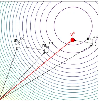
In PSO, the first step is to randomly position a swarm composed of several particles in the misfit landscape (i.e. model parameter space). Each particle represents a model and can be seen as flying through the misfit landscape while interacting with its neighborhood to find the global minimum of the misfit function. Neighborhood topologies are more thoroughly described in Section2.2.2. All along the optimization process, each particle remembers the best position it has visited so far in addition to the best position achieved by the entire swarm. More specifically, a particle i is defined by a position vector mk
i and a velocity vector vki which is adjusted according
to its own personal best position and the global best position of the whole swarm. The velocity and the position of each particle are updated following
vki = !vk−i 1+ ffiprkp “ mp;i− mk−i 1 ” + ffigrkg “ mg − mk−i 1 ” (2.6) mki = mk−i 1+ v k i (2.7)
where mp;i and mg are respectively the personal best position of particle i and the global best
position of the population, rk
p and rkg are uniform random number vectors drawn at iteration k,
! is an inertia weight, ffipand ffig are two acceleration parameters that respectively control the
cognition and social interactions of the particles. Principle of PSO is illustrated in Figure2.6.
mg mik-2 mik-1 mp,i mik vik
Figure 2.6:Principle of PSO on a 2D misfit function represented by the contour lines. Particle velocity vk i is constructed by adding three weighted terms: the previous velocity vk−1
i that acts as an inertial term, the cognition term“mp;i − mki−1” that accounts for the particle’s personal knowledge, and the sociability term“mg− mki−1” that involves the knowledge of the entire swarm.
The inertia weight ! has been introduced by Shi and Eberhart (1998) to help the particles to dynamically adjust their velocities and refine the search near a local minimum. Another formulation using a constriction coefficient based on Clerc (1999) to insure the convergence of the algorithm can be found in the literature. However, Eberhart and Shi (2000) showed that the inertia and constriction approaches are equivalent since the parameters are connected.
Empirical works have concluded that the performance of PSO is sensitive to its control param-eters, namely the swarm size n, the maximum number of iterations kmax, !, ffip and ffig. Yet,
these studies have provided some insights on the initialization of some parameters (Van Den Bergh and Engelbrecht (2006)). Eberhart and Shi (2000) empirically found that ! = 0:7298 and
ffip= ffig = 1:49618are good parameter choices that lead to convergent behavior.
The swarm size and the maximum number of iterations have to be carefully chosen depending on the problem and the computer resources available. These two parameters are related since a smaller swarm requires more iterations to converge, while a bigger swarm converges more rapidly. In real-world optimization problems, the computation cost is mainly dominated by the forward modeling. Therefore, the optimization is usually stopped when a predefined number of forward modelings (i.e. computations of misfit functions) is performed. The desired number of forward modelings is controlled by both the swarm size and the maximum number of iterations. Trelea (2003) has studied the effect of the swarm size on several benchmark test functions in 30 dimensions. He found that a medium number of particles (≈ 30 particles) gives the best results in terms of number of misfit function evaluations. Too few particles (≈ 15 particles) gives a very low success rate while too many particles (≈ 60 particles) results in much more misfit function evaluations than needed although it increases the success rate. Piccand, O’Neill and Walker (2008) came to the same conclusion with problems of higher dimensions (up to 500).
Constraints handling
Empirical studies have shown that the particles are prone to go beyond the search space boundaries early throughout the optimization process. This behavior can raise several possible problems such as
• Infeasible optimal solution: as personal best positions are pulled outside of the search space, the global best position is pulled outside of the feasible space as well;
• Wasted effort: if particles fail to find a better solution outside, they are eventually pulled back into the feasible space;
• Divergence: particle’s velocity increases drastically as the particle is distant from its personal best and global best.
Several strategies that act directly upon the velocity have been proposed to address this behavior. For instance, the velocity vector can be clamped to lie in [−Vmax; Vmax] to keep the particle
from moving too far from the model parameter space (Clerc and Kennedy (2002), Van Den Bergh and Engelbrecht (2006)). However, Angeline (1998) showed that velocity clamping is not sufficient to properly control the step size. Besides, the optimal clamping threshold Vmax is
problem-dependent. Another factor that can potentially influence the performance of PSO is how velocities are initialized. Engelbrecht (2012) demonstrated that particles tend to leave the search space independently of the velocity initialization approach and that the best approach is to initialize particles to zero.
Therefore, it may be required to constrain the particles to stay within the feasible space by repairing infeasible solutions. Several approaches are available in the literature of evolutionary algorithms, such as:
• Random: this approach is the most common and simply consists in resampling each parameter of a solution that violates the feasible space boundaries, as shown in Figure2.7 (left);