Bayesian Mixtures of Triangular distributions with application to Goodness-of-Fit Testing

(1)

WITH APPLICATION TO GOODNESS-OF-FIT TESTING

R.MCVINISH, J. ROUSSEAU, AND K. MENGERSEN

Abstract. Two forms of mixtures of triangular distributions are considered as an alternative to the Bernstein polynomials for Bayesian nonparametric density estimation on [0,1]. Conditions for weak and strong consistency of the posterior distribution and a rate of convergence are established. This class of priors is applied to the problem of testing a parametric family against a nonparametric alternative.

1. Introduction

The Bernstein polynomial prior for nonparametric density estimation on [0, 1] has been studied by Petrone (1999a,b), Ghoshal (2001) and Petrone and Wasserman (2002). Perron and Mengersen (2001) have shown that the Bernstein polynomials are a poor approximation to the space of distribution functions on [0, 1]. A better approximation can be achieved by mixtures of Triangular distributions.

For a given k ≥ 1, let the sequence 0 = x−1 = x0 < x1 < . . . < xk−1 < xk =

xk+1 = 1 be a partition of [0, 1]. The function hi(x) is the triangular density

function with support on the interval [x_i−1, xi+1] and mode at xi. The mixture of

triangular distributions has the density function p (x) =

k

X

i=0

wihi(x) ,

where wi ≥ 0, Pk_i=0wi = 1. Note that p (x) is a piecewise linear function on [0, 1]

interpolating the points (xi, wihi(xi)) . The two cases considered by Perron and

Mengersen (2001) were:

Date: June 14, 2005.

1991 Mathematics Subject Classification. Primary: 62C10 Secondary: 62G07, 62F15. Key words and phrases. Bayesian nonparametrics, consistency, goodness-of-fit.

This work was supported by the ARC Center of Excellence - Center for Complex Dynamical Systems and Control CEO348165.

(2)

I For each k, the partition of [0, 1] is assumed fixed and the weights wi are to

be estimated.

II For each k, the weights wiare fixed at w0= wk = _2k1 , wi= _k1, i = 1, . . . , k−1

and the partition is to be estimated.

The advantage of these Triangular distributions as priors is that they are both simple and flexible. In particular their implementation is quite straightforward, see Perron and Mengersen (2001). On the other hand they provide a good approxima-tion to smooth densities, so that the posteriors associated with these priors have good frequentist asymptotic properties. We prove in particular that they lead to minimax estimators of the densities for some class of densities, see Section 2.

In this paper we study the asymptotic properties of the posterior distributions associated with these priors, which leads to the asymptotic properties of the related Bayes estimators. We also construct Goodness of fit tests using these priors. We first study the asymptotic behaviour of the Bayes factor since it is widely used as a test statistic in the Bayesian community. To begin with we consider the simple test against a fixed known distribution, which is equivalent to testing against the uniform. In this case consistency of the Bayes factor is proved under very general conditions and rates of convergence are obtained which are as anticipated: n−1/2 under the null hypothesis and exponential rates for fixed alternatives. These results are stated in Section 3. We then extend our results to testing against a parametric model Q = {pθ, θ ∈ Θ}. This is a widely studied problem, see for example Zhang

(2002), Fortiana and Grane (2003), Munk and Czado (1998) and references therein. Here instead of embedding the parametric family into a nonparametric family as was done by Florens, Richard and Rolin (1996), Carota and Parmigiani (1996), Berger and Guglielmi (2001) and Verdinelli and Wasserman (1998) we consider the test of the parametric family (which is considered as a distribution on [0, 1] without loss of generality) against the nonparametric model defined by the mixture of triangular densities. This has the advantage of substantial simplification of the models but we show that it has limitations with respect to the Bayes factor. Indeed, we prove that if both models are separated enough, in other words if no density of the parametric family can be represented exactly by a finite mixture of triangular density, then the Bayes factor is consistent; otherwise it is not consistent. Bayes factors are to some extent the Bayesian answers to 0-1 types of losses. Goodness of fit tests are seldom phrased as such; the question is rather whether the true density can be reasonably

(3)

well represented by a parametric family of densities. Therefore, we also propose another test based on a distance approach, similar to that considered by Robert and Rousseau (2004). This is the Bayesian solution to the loss function function defined by, for any density p on [0, 1]

L(δ, p) = (

a0d(p, Q) if δ = 0

a1(1 − d(p, Q)) if δ = 1

(1.1)

where d(p, Q) = infθ∈Θd(p, pθ) and d(p, pθ) = R₀1|p(x) − pθ(x)|dx. The Bayes

es-timator is then given by δ(Yn) = 0 (we accept the parametric family) if and only if

T (Yn) = Eπ[d(p, F)|Yn] ≤ a1/(a0+ a1),

where Yn_{= (Y}

1, ..., Yn) is the vector of observations. Since the choice of (a0, a1) is

often arbitrary we propose, as in Robert and Rousseau (2004), to calibrate the test procedure using a Bayesian p-value, namely the conditional predictive p-value pcpred

based on the maximum likelihood estimator under the parametric family: let ˆθ be the maximum likelihood estimator based on the observations Yn

pcpred(ˆθ, Yn) = Z Θ Pθ h T (Xn) > T (Yn_{)| T (Y}n), ˆθiπ0(θ|ˆθ)dθ.

This p-value has been proposed by Bayarri and Berger (2000) and discussed by Robbins et al. (2000), Robert and Rousseau (2004) and Fraser and Rousseau (2005). In Section 4.3 we study the asymptotic behaviour of this test procedure and we prove that it is also optimal in the frequentist sense.

The following section states the consistency results for these mixtures. Since the methods of proof for the first case of mixtures are very similar to that of the Bernstein polynomials, the proofs will be omitted or sketched. For both cases of mixtures the resulting density estimates can be shown to converge at the minimax rate for H¨older continuous density functions, up to a (log n) term. This rate of convergence is significantly faster than for the Bernstein polynomials.

2. Asymptotic properties of the posterior distributions

We first give some definitions that will be used throughout this paper. The most common measures of distance between two densities p, q are the L1-distance, denoted

by k p − q k1, and the Hellinger distance h (p, q) =k p1/2− q1/2 k2. We allow d to

stand for either of these distances. The Kullback-Leibler divergence is defined by K (p, q) =Rlog(p/q)p dµ and let V (p, q) =R log(p/q)2p dµ. The space of densities

(4)

will be denoted by F. The prior on F is denoted by π and the posterior distribution given data Yn= (Y1, . . . , Yn) is denoted by π (· | Yn). The true distribution function

is denoted by P0 and its density by p0.

2.1. Type I mixture. For the Type I mixture of triangular distributions the par-tition on [0, 1] is defined as xi = i/k, i = 0, 1, . . . , k. This choice of partition is

made for simplicity. Alternative partitions could be more suitable to different den-sity functions. The prior for these mixtures is assumed to satisfy the following basic assumptions:

• For all k = 1, 2, . . . π (k) > 0

• Given k, the support of the prior on w = (w0, . . . , wk) is the entire

k-dimensional simplex. Hence, for any set U of positive Lebesgue measure π (U | k) > 0.

The aim of this subsection is to give sufficient conditions on the prior leading to a given rate of convergence for the posterior. This result will play a significant role in the later discussions on goodness-of-fit testing. In the process we shall recall some theorems used in proving convergence of the posterior. As with the Bernstein polynomial priors, for a given k, this first class of mixtures is a simple convex combination of density functions which are bounded by a multiple of k. Thus the following theorems can be proved using very similar techniques to those used in the corresponding theorems for Bernstein polynomials(Petrone and Wasserman (2002), Ghosal (2001)). Hence the proofs of this section will either be omitted or sketched. Consider first weak consistency of the posterior distribution, that is the posterior probability of all weak neighbourhoods of the true density converges to one, almost surely. Since this is sufficient for the posterior predictive distribution function to converge weakly to the true distribution function. Hjort (2003) argues that this is sufficient for most inferential questions. Schwartz (1965) established the following sufficient condition for weak consistency of the posterior. See Walker (2003) for a different proof.

Theorem 2.1 (Schwartz (1965)). If the prior places positive probability on every Kullback-Leibler neighbourhood of p0 then the posterior is weakly consistent at p0,

almost surely.

The proof of the following theorem requires only very minor modifications to the proof of Theorem 2 in Petrone and Wasserman (2002).

(5)

Theorem 2.2. Suppose P0 has a continuous density p0on [0, 1]. If the prior satisfies

the above assumption then the resulting posterior is weakly consistent at P0.

Often we are interested not only in functionals of the posterior predictive den-sity but also in an estimate of the denden-sity function. It is well known that weak convergence of a distribution does not imply convergence of the respective density function without additional conditions on the prior. For the posterior predictive den-sity to converge to the true denden-sity, with respect to the L1 or Hellinger distances,

it is sufficient to show that the posterior probability of all strong (i.e. Hellinger) neighbourhoods of the true density converge to one, almost surely (Ghosh and Ra-mamoorthi (2003), proposition 4.2.1). Sufficient conditions for strong consistency of the posterior distribution have been established by Baron et al. (1999), Ghosh and Ramamoorthi (2003) and Walker (2004). For a subset A of F and δ > 0 let D (δ, A, d) denote the minimum number of points in A such that the distance between each pair is no greater than δ, sometimes called the δ-covering number. Theorem 2.3 (Ghosh and Ramamoorthi (2003), Theorem 4.4.4). Let π be a prior on F. Suppose the conditions of Theorem 2.1 are satisfied. If for each ǫ > 0, there is a δ < ǫ, c1, c2 > 0, β < ǫ2/2, and Fn⊂ F such that, for all n large,

• π (Fnc) < c1e−nc2,

• log D (δ, Fn, |·|) < nβ,

then the posterior is strongly consistent at p0.

The following theorem may be proved by a minor modification of the proof of theorem 3 in Petrone and Wasserman (2002).

Theorem 2.4. Suppose there exists kn−→ ∞ such that kn= O (n) andP_k≥k_nπ (k)

≤ exp (−nr) for some r > 0. Further suppose that the assumptions of Theorem 2.2 hold. Then the resulting posterior is Hellinger consistent at P0.

Ghosal (2001) showed that under certain conditions the rate of convergence of the posterior distribution from a Bernstein polynomial prior is of the order n−1/3(log n)5/6 provided the true density is bounded away from zero and has a bounded second derivative. This rate is much slower than can be achieved by other methods, though is believed to be sharp except for the (log n) term. Theorem 2.3 in Ghosal (2001) can be adapted to determine the rate of convergence of the posterior

(6)

for mixtures of triangulars. The conditions that need to be checked are given by Ghosal’s Theorem 2.1 which is stated below.

Theorem 2.5 (Ghosal (2001) Theorem 2.1). Let πn be a sequence of priors on F.

Suppose that for positive sequences ¯ǫn, ˜ǫn−→ 0 with n min

¡ ¯

ǫ2_n, ˜ǫ2_n¢_{−→ ∞, constants} c1, . . . , c4> 0 and sets Fn⊂ F, we have

log D (˜ǫn, Fn, d) ≤ c1n¯ǫ2n, (2.1) πn(Fnc) ≤ c3e−(c2+4)n˜ǫ 2 n_, (2.2) πn(N (˜ǫn, p0)) ≥ c4e−c2n˜ǫ 2 n_, (2.3)

where N (ǫ, p0) = ©p : K (p0, p) < ǫ2, V (p0, p) < ǫ2ª. Then for ǫn = max (¯ǫn, ˜ǫn)

and a sufficiently large M > 0, the posterior probability (2.4) πn(p : d (p, p0) > M ǫn| Yn) −→ 0,

in P₀n-probability.

Theorem 2.6. Assume that p0 belongs to the H¨older class H(L, β), with β, L > 0

and satisfies p0(x) ≥ ax(1 − x) for some constant a > 0. Assume the Type I mixture

of triangular distributions prior for p satisfies b1e−β1k ≤ π (k) ≤ b2e−β2k for all k

for some constants b1, b2, β1, β2 > 0 and for each k the prior on w is a Dirichlet

distribution with parameters bounded for all k. Then for a sufficiently large constant M , • If β ≤ 2 then E0[Π ³ p : d (p, p0) > M n−β/(2β+1)(log n) | Yn ´ ] ≤ n−H, _{∀H > 0,} when n is large enough.

• If β > 2 then E0 h Π³p : d (p, p0) > M n−2/5(log n) | Yn ´i ≤ n−H, _{∀H > 0,} when n is large enough.

Proof. Assume initially that β ≤ 2; the case of β > 2 follows exactly the same lines. Let C denote a generic finite, positive constant which may be different in each instance. First, define the function p (x; ˆw0, k) by

(7)

where p0_i = p0(i/k) for k − 1 ≥ i ≥ 1 and if p0(0) = 0, (resp. p0(1) = 0) p00 =

k−β_{∧ p}0(1/k) else p00 = P0(0) (resp. p0k = k−β∧ p0(1 − 1/k) else pk0 = p0(1)). It is

easily seen that the density defined by p (x; w0, k) = p (x; ˆw0, k) /S, with S = (p0+

pk)/(2k) +Pk−1_i=1 pi/k is a mixture of triangular densities. The function p (x; ˆw0, k)

is, with minor modification at x = 0 and x = 1, simply the linear interpolation of p0 so sup_0≤x≤1|p0(x) − p (x; ˆw0, k)| ≤ Ck−β. It follows that S = 1 + O

¡ k−β¢ and sup_0≤x≤1_|p0(x) − p (x; w0, k)| ≤ Ck−β. Then the Kullback-Leibler distance

between p0 and pw is bounded by

K(p0, p (.; w0, k)) ≤

Z _{(p (x; w}

0, k) − p0(x))2

p (x; w0, k)

dx. This implies that

K(p0, p (.; w0, k)) ≤ (1 − S)2+ Ck−2β−1 k−2 X i=1 p (x; ˆw0, k)−1 +Ck−2β−1 ÃZ 1 0 u2 (p1₀+ up0₀)du + Z 1 0 u2 (pk−1₀ + upk 0) du ! ≤ (1 − S)2+ Ck−2βlog k.

Therefore, if k w0 − w k1≤ ǫ1+1/β| log ǫ|−1/2(1+1/β) and d1ǫ−1| log ǫ|1/2 ≤ kβ ≤

d2ǫ−1| log ǫ|1/2 for some constants d1, d2 then

sup

0≤x≤1|p0(x) − p (x; w, k)| ≤ Cǫ| log ǫ| −1/2_.

For ǫ small enough p (x; w, k) will be bounded away from zero on [1/k, 1 − 1/k] and near the boundary p (x; w, k) ≥ ck−β _{for some constant c > 0. It follows that}

sup_x_|p0(x) − p (x; w, k) | ≤ Ck−β and we can apply the same calculations as with

p (x; w0, k) so that p (x; w, k) ∈ N (Cǫ, p0) and hence n p (x; w0, k) : kw − w0k1 ≤ ǫ1+1/β| log ǫ|−1/2(1+1/β) o ⊂ N (Cǫ, p0) .

(8)

Now let ǫ depend on n by taking ˜ǫn= n−β/(2β+1)(log n)1/2 and let

d1n1/(2β+1)≤ kn≤ d2n1/(2β+1),

for constants d1, d2. Applying lemma A.1 of Ghosal (2001) gives

π (N (C˜ǫn, p0)) ≥ Ce−cknlog(1/˜ǫn),

and thus condition (2.3) is satisfied.

Define the sets Fn = {p (·; w, k) : k ≤ sn}, i.e. those mixtures with sn or less

components. The condition (2.2) of Theorem 2.5 is satisfied by taking sn to be an

integer satisfying

d1n1/(2β+1)(log n) ≤ sn≤ d2n1/(2β+1)(log n) ,

as π (Fc

n) ≤ Ce−cn˜ǫ

2

n where c can be made arbitrarily large by taking d₁ sufficiently

large. Finally, to check the condition (2.1) we follow the arguments in Ghosal’s Theorem 2.3 and note that log D (ǫ, Fn, d) is bounded by

snlog µ C ǫ ¶ + log sn.

Upon taking ¯ǫn= n−β/(2β+1)(log n) condition (2.1) is satisfied. Note that Theorem

2.5 only gives convergence in probability. However the bound on the expectation of the posterior probability as given in Theorem 2.6 comes from their proof and from the fact that when p (·; w, k) is considered as above,

P₀n£log p(Yn_{) − log p}0(Yn) ≤ −nCǫ2¤ ≤ e−snCǫ

2³

E0

h

es log (p0/p)(Y )i´n

≤ Cn−H, when n is large enough and ǫ2 _{≤ ǫ}

0n−2β/(2β+1), by choosing correctly s. This implies

using Shen and Wasserman (2001)’s type of proof that P₀n ·Z _p(Yn_{; w, k)} p0(Yn) dπ(w, k) ≤ e −2nCǫ2 n ¸ ≤ n−H

for all H > 0, when n is large enough. This completes the proof. ¤ This Theorem implies in particular that if ˆp(x) = Eπ_{[ p(x)| Y}n], then when n is large enough,

E₀n[d(ˆp, p0)] ≤ 2Cn−β/(2β+1)(log n),

which is the minimax rate of convergence for the class of H¨older continuous functions H (β, L) (up to a log n term).

(9)

The assumption of p0(x) ≥ ax(1 − x) in Theorem 2.6 can be removed at the

expense of having a slower rate of convergence. Without the lower bound on p0

a small modification of the above proof will yield a rate of convergence, up to a (log n), of n−β/(2β+2)_{. While this is significantly slower than the minimax rate, it is}

the same as that achieved by the Bernstein polynomials (Ghosal (2001)) for twice differentiable densities and will be sufficient for our examination of the Bayes factor in section 4.1.

Simulating from the posterior distribution with a fixed number of components poses no difficulty. Using a Dirichlet prior on the weights associated with each component in the mixture, a two-stage Gibbs sampling strategy can be implemented by taking advantage of the usual latent variable structure;

zi ∼ M (w0, . . . , wk) , Yi | zi, k ∼ hzi(y) ,

where M is the multinomial distribution and if zi has a 1 in the j-th position then

hzi is the triangular density hj as described in the introduction.

We need to deal with the case of an unknown number of components in the mixture. Two prominent approaches to the problem are Richardson and Greens (1997) reversible jump MCMC algorithm and the birth-and-death process described in Stephens (2000). The lack of a nested structure in these mixtures makes the construction of suitable proposal distributions difficult. The approach adopted in this paper will be to simulate from the posterior conditional on the number of components and then determine posterior probability for the number of components using the marginal likelihood calculations described in Chib (1995). Given k, the marginal likelihood m(y | k) is computed from the Gibbs output {z1, ..., zM} as

log ˆ_{m (y | k) = log f (y | w}∗, k) + log π (w∗ _{| k) − log} ( M−1 M X i=1 π (w∗_{| y, z}j, k) )

for a suitable w∗ _{such as the posterior mode.}

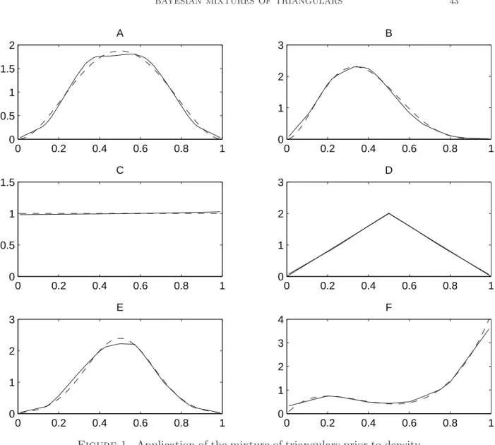
These computations are demonstrated on a small collection of simulated data sets. The data comprise 1000 independent realizations from each one of the following six densities: (A) Beta(3,3), (B) Beta(3,5), (C) Uniform, (D) Triangular, (E) Truncated Normal(1/2,1/36), and (F) 0.3×Beta(2,5) + 0.7×Beta(6,1). In each case a geometric distribution with parameter 0.6 was taken for the prior on the number of components k in the mixture (truncated at k = 10). Given k, a Dirichlet prior was placed on

(10)

the weights with parameters (4/(k + 1), ..., 4/(k + 1)). The posterior mean density estimates are plotted in Figure 1.

Figure 1 near here.

2.2. Type II Mixtures. The type II mixture is slightly more complicated to study than the type I, in the same way as the free knot splines are more complicated to study than fixed splines estimators. However here, the problem is made easier since the weights are fixed. In this section we study the asymptotic properties of the posterior distributions associated with type II mixtures and give sufficient conditions for consistency.

The following assumptions on the prior for the mixture of triangular distributions are made:

• For all k = 1, 2, . . . π (k) > 0.

• Given k, the support of the prior on the partition increments {x1− x0, x2− x1, . . . , xk− xk−1}

is the entire k-dimensional simplex. Hence, for any set U of positive Lebesgue measure, π (U | k) > 0.

These conditions on the prior are sufficient to establish weak consistency when p0 is continuous.

Theorem 2.7. Suppose p0 is a continuous density on [0, 1]. The Type II mixture

of triangular distributions posterior is weakly consistent at p0.

Proof. From Schwartz’s theorem we only need to check that every Kullback-Leibler neighbourhood of any continuous density function has positive prior probability. It is initially assumed that

inf

x∈[0,1]p0(x) = a > 0.

We now show that any continuous density on [0, 1] that is bounded away from zero can be uniformly approximated by a sequence of mixtures of triangular densities p_ψ(k), where ψ(k) denotes a partition of size k. For a given k the partition

ψ(k) = {x0, x1, . . . , xk}

of [0, 1] is chosen to satisfy the equations P0(xi) = i/k, i = 0, . . . , k. From the mean

value theorem

(11)

for i = 1, . . . , k − 1. For i = 0, k

P0(x1) − P0(x0) = 1/k = p0(x∗0) (x1− x0) , x∗0∈ (x1, x0) ,

P0(xk) − P0(xk−1) = 1/k = p0(x∗k) (xk− xk−1) , x∗k∈ (xk−1, xk) .

It follows that pψ(k)is the linear interpolation of the points (xi, p0(x∗i)) , i = 0, . . . , k.

Take any x ∈ (xi, xi+1), the density pψ(k)in this interval is given by

pψ(k)(x) = p0¡x∗i+1 ¢ − p0(x∗i) xi+1− xi (x − xi ) + p0(x∗i) . and hence ¯ ¯p0(x) − pψ(k)(x) ¯ ¯ ≤ |p0(x) − p0(x∗i)| + ¯ ¯p0(x∗i) − pψ(k)(x) ¯ ¯ ≤ |p0(x) − p0(x∗i)| + ¯ ¯p0 ¡ x∗_i+1¢_{− p}0(x∗i) ¯ ¯ x − xi xi+1− xi . We note that 1 M k ≤ |xi− xi−1| ≤ 1 ak,

where M = sup_x∈[0,1]p0(x). As a continuous function on [0, 1] is uniformly

continu-ous it follows that any continucontinu-ous density bounded away from zero can be uniformly approximately by a mixture of triangular densities. Similar arguments to those used by Petrone and Wasserman (2002) in the proof of their Theorem 2 can be applied to conclude that lim k−→∞ Z log · p0(x) p_ψ(k)(x) ¸ p0(x) dx = Z lim k−→∞ µ log · p0(x) p_ψ(k)(x) ¸ p0(x) ¶ dx = 0. Thus, for any δ there exists an k0 such that for all k > k0, K

¡

p0, pψ(k)

¢ < δ.

Now consider k to be fixed and so we denote ψ(k) by ψ. Let η = (x0, ˜x1, . . . , ˜xk−1, xk)

and for ǫ > 0 define the neighbourhood around ψ by Nǫ = ½ η : max j=1,...,k|˜xj− xj| < ǫ kM ¾ . We aim to show that for η ∈ Nǫ,

lim

η−→ψK (p0, pη) −→ K (p0, pψ) .

From lemma 6.1

sup

x∈[0,1]|pψ(x) − pη(x)| ≤ CMǫ

(12)

Again, following similar arguments to Theorem 2 of Petrone and Wasserman (2002) it follows that K (p0, pη) is continuous in η at ψ. Hence, for any δ we can

choose an ǫ such that K (p0, pη) < δ for any η ∈ Nǫ. Therefore, the prior probability

on any Kullback-Leibler neighbourhood of a continuous density function bounded away from zero is strictly positive. The condition that inf_x∈[0,1]p0(x) = a > 0 can

be removed using lemma 6.3.2 of Ghosh and Ramamoorthi (2003). ¤ It was noted in Perron and Mengersen (2001) that any continuous distribution function can be well approximated by a finite Type II mixture of triangular distri-butions. This was in contrast to Type I mixtures of triangular distributions and the Bernstein polynomials which could perform poorly, particular for non-differentiable distribution functions. The ability of Type II mixtures to always approximate a con-tinuous distribution function well arise as these mixtures can place a large amount of probability on rather small intervals. Such behaviour, while being advantageous in the context studied in Perron and Mengersen (2001), poses a difficulty for consistent density estimation as for any given k > 3 the set of Type II mixtures has an infinite δ-covering number. For this let p1, . . . , pm be any finite collection of densities on

[0, 1] and let pη(k)be a mixture of triangular densities. For |x3− x1| in the partition

η(k) sufficiently small the distance between p_η(k) and pi will be greater than 1/k

for any i = 1, . . . , m. Hence, the δ-covering number is infinite for any δ < 1/k. To overcome this the prior needs to be formed so that the prior probability of any points in the partition being close to each other is very small. The precise statement of this is given in the following theorem.

Theorem 2.8. Assume that the prior satisfies,

• The prior on the number of components k is such that π (k > n/(log n)) ≤ e−nr.

• Given k, the prior places very small probability on two points in the partition being close. Specifically, π (|xi− xi−1| < n−a| k) < e−nr,

for some a, r > 0 and all n sufficiently large. Suppose p0 is a continuous density on

[0, 1]. The Type II mixture of triangular distributions posterior is strongly consistent at p0.

Proof. Strong consistency of the posterior is proved by checking the conditions stated in Theorem 2.3 hold. From Theorem 2.7 we have that under these conditions any continuous probability density function is in the Kullback-Leibler support of the

(13)

prior. For a given k consider the set formed by the collection of all partitions ψ(k) of [0, 1] such that sup_x∈[0,1]p_ψ(k)_{(x) ≤ n}a _{and define F}n to be the union of these

sets for k = 1, . . . , kn, i.e.

Fn= kn [ k=1 ( ψ(k) : sup x∈[0,1] p_ψ(k)_{(x) ≤ n}a ) . The prior probability on Fc

n needs to decrease exponentially quickly.

π (Fnc) = π ({k > kn}) + kn X k=1 π Ã( ψ(k) : sup x∈[0,1] p_ψ(k)(x) > na )! ≤ π ({k > kn}) + kn X k=1 π µ½ ψ(k) : min i |xi− xi−1| < n −a ¾¶

The assumptions made on the prior will ensure that with the appropriate choice of kn = k0n/(log n), π (Fnc) < Ce−nc for some c and all sufficiently large n. Now to

show that the L1 δ-covering number of Fn grows at the correct rate. Consider for

a fixed k, two mixtures of triangular distributions pψ and pη which are bounded by

M . From Lemma 6.1 if k ψ − η k(∞)≤ CkMδ 2 then k pψ− pη k(1)≤ δ. The number of

density functions required to cover nψ(k) : sup_x∈[0,1]pψ(k)(x) ≤ na

o is then µ Ckn2a δ ¶k

and hence to cover Fn we need

kn

µ

Cknn2a

δ

¶kn

density functions. The L1 entropy is then

log D (δ, Fn, k · k1) = kn¡2a log n + log kn+ log δ−1+ log C¢.

Letting kn= k0n/(log n) we have log D (δ, Fn, k · k1) < nk0(2a + 1), for sufficiently

large n and hence, if k0 < ǫ2/(2a + 1) the conditions of Theorem 2.3 are satisfied.

It follows now that the posterior is strongly consistent at p0. ¤

As in the case of fixed partition and free weights we obtain the minimax rate of convergence up to a log n term. The result is presented in the following theorem. Theorem 2.9. Assume that the true density p0 belongs to the H˝older class H(β, L)

with regularity β. Assume also that p0 ≥ a > 0 on [0, 1]. In addition, assume that

(14)

• The prior on the number of components k is such that there exists c1, c2 > 0

satisfying e−c1n log n _{≤ π (k > n) ≤ e}−c2n log n _{for all n sufficiently large.}

• Given k, the prior places very small probability on two points in the partition being close. Specifically, π (|xi− xi−1| < n−a| k) < e−rn, for some a, r > 0

and all n sufficiently large. Then there exists C > 0 such that

E₀nhΠ³pψ : d (pψ, p0) > Cn−β/(2β+1)log n ¯ ¯ ¯ Yn ´i ≤ n−H, _{∀H > 0,} when n is large enough.

Proof. The proof follows the line of the proof on the strong consistency. If β ≤ 1, using the construction of p_ψ(k), ψ(k) = (x1, ..., xk−1) described in Theorem 2.6, we

obtain that

|p0− pψ(k)|∞≤ Ck−β, if p0 ≥ a > 0.

If β ∈ [1, 2], we note that for each i ≤ k − 1, p0(x) = p0(xi) + (x − xi

) xi+1− xi

(p0(xi+1) − p0(xi)) + O(k−β).

Therefore, for x ∈ (xi, xi+1)

|p0− pψ(k)| = ¯ ¯ ¯ ¯(p0(xi) − p0(x⋆i)) (xi+1− x) xi+1− xi + (p0(xi+1) − p0(x⋆i+1)) (x − xi ) xi+1− xi ¯ ¯ ¯ ¯ . We also have, using a Taylor expansion of Rxi+1

xi p0(x)dx and of

Rxi

xi−1p0(x)dx, both

equal to 1/k:

p0(xi)[(xi+1− xi) − (xi− xi−1)]

= −p′0(xi)[(xi+1− xi)2+ (xi− xi−1)2]/2 + O(k−β−1)

= O(k−2),

and using a Taylor expansion ofRxi+1

xi−1 p0(x)dx, p0(x⋆i)(xi+1− xi−1) = p0(xi)(xi+1− xi−1) + p0(xi)′ 2 [(xi+1− xi) 2 − (xi− xi−1)2] + O(k−β−1),

which implies that

(15)

The same argument can be applied to show p0(xi) − p0(x⋆_i) = O(k−β). Therefore,

the absolute difference of p0 and pψ(k) is bounded by Ck−β for some C > 0. Let

η(k) be another partition and p_η(k) the resulting density. From Lemma 6.1 we have |p0(x) − pη(k)(x) | ≤ C(k−β+ ǫ),

where |ψ(k) − η(k)| < cǫk−1. Taking k to satisfy d1ǫ−1 < kβ < d2ǫ−1 for constants

d1, d2 and applying Lemma 8.2 of Ghosal et al. (2000) it is seen that

N (Cǫ, p0) ⊃

©

η(k) : |η(k) − ψ(k)| < cǫk−1ª Allow k to depend on n by taking

d1 µ n log n ¶1/(2β+1) ≤ kn≤ d2 µ n log n ¶1/(2β+1)

and ˜ǫn= kn−β. The prior probability on N (C˜ǫn, p0) can be bounded below

π(Nǫn) ≥ π(κn)πκn[η : |˜xi− xi| ≤ ǫn/(M κn)]

≥ π(κn)Γ(κn) (cǫn/κn)

κn−1

Γ(κn/2)

≥ Cec1n1/(2β+1)log n_,

for some constants c, c1, C > 0. Hence, condition (2.3) of Theorem 2.4 is satisfied.

Similar to Theorem 2.7 define Fn= kn [ k=1 ( η(k) : sup x∈[0,1] p_η(k)_{(x) ≤ n}a/(2β+1) ) .

Under the assumptions of this theorem π (Fc

n) ≤ Ce−cn

1/(2β+1)_{log n}

, and so condition (2.2) is satisfied. Finally, the entropy is obtained using the same calculations as Theorem 2.7, replacing δ by ǫn. This leads to the L1 entropy being bounded from

above by Cn1/(2β+1)_{log n. Taking ǫ}

n = n−β/(2β+1)(log n)β/(2β+1) condition (2.1) is

satisfied and the proof is achieved. _¤

Calculations can be performed by Metropolis-Hastings sampling for fixed k and marginal likelihoods calculated from the output as described in Chib and Jeliazkov (2001). We see from this section that mixtures of triangulars are an easy and efficient tool for density estimation. It is in particular adaptive for β at least in the range β ≤ 2. In the next section we use these priors in a different context than estimation, namely testing.

(16)

3. Application to Goodness-of-Fit Testing - Point Null Hypothesis Now consider the problem of testing the point null hypothesis that the data Yn belong to some completely specified distribution. Without loss of generality, this distribution is assumed to be uniform on [0, 1]. The alternative hypothesis is that the data belong to some distribution with a continuous density function, other than the uniform.

H0: Y1, . . . , Yn are independent observations from a U (0, 1) distribution.

H1: Y1, . . . , Yn are independent observations from a distribution with a

continu-ous density p0 (not uniform).

Verdinelli and Wasserman (1998) modeled the density in H1 with an infinite

di-mensional exponential family in testing the above hypothesis. In their Theorem 8.1, Verdinelli and Wasserman (1998) show that under rather strong conditions the Bayes factor defined by

Bn= Pr (H0 | Y1, . . . , Yn) Pr (H1 | Y1, . . . , Yn)÷ Pr (H0) Pr (H1) = (Z Ω n Y i=1 p (Yi) π (dp) )₋₁

is consistent. The following is an improvement and generalization of their result. Theorem 3.1. Assume that the prior on the density in H1 places positive

proba-bility on all Kullback-Leibler neighbourhoods of all continuous density functions. In addition, assume that this prior places zero probability on the uniform density.

(i) If H1 is true then Bn−→ 0 exponentially quickly, almost surely with respect

to P∞_.

(ii) If H0 is true then Bn−1−→ 0, almost surely with respect to P∞.

Proof. The proof of (i) is the same as the proof of Theorem 8.1 (i) in Verdinelli and Wasserman (1998). For part (ii) we first show that B−1

n forms a martingale.

Applying Fubini’s theorem

E£B_n+1−1 _{| Y}n, . . . , Y1 ¤ = Z ΩE "_n+1 Y i=1 p (Yi) | Yn, . . . , Y1 # π (dp) = Z ΩE [p (Yn+1 )] n Y i=1 p (Yi) π (dp) = B_n−1.

(17)

Similarly, E¡B₁−1¢ = 1 and hence B_n−1 is a martingale with respect to the filtra-tion σ (Yn, . . . , Y1). Using Doob’s Theorem on non-negative (sub)martingales, since

E(B−1

n ) = 1 < ∞, there exists an integrable random variable X∞ such that as

n −→ ∞, B−1

n −→ B∞−1, P∞ almost surely.

Now let V be a weak neighbourhood of the uniform distribution which we shall denote by P0. Specifically, let m be some arbitrary but finite integer, ǫj > 0, fj, j =

1, . . . , m be bounded continuous functions and define V as

V = m \ j=1 ½ P : ¯ ¯ ¯ ¯ Z fjdP − Z fjdP0 ¯ ¯ ¯ ¯ < ǫj ¾ = m \ j=1 ½½ P : Z fjdP − Z fjdP0 < ǫj ¾ \ ½ P : Z fjdP0− Z fjdP < ǫj ¾¾

We can then write

B_n−1 = Z V + Z Vc n Y i=1 p (Yi) π (dp) = I1+ I2

Fix a > 0. We can apply Markov’s inequality and then the Fubini theorem to I1 to

get Pr ÃZ V n Y i=1 p (Yi) π (dp) > a ! ≤ a−1π (V )

For I2 let U be one of the sets in the finite intersection forming the set V . There

exists a strictly unbiased function for testing P = P0 versus P ∈ Uc and so by

proposition 4.4.1 in Ghosh and Ramamoorthi (2003) there also exists a uniformly exponentially consistent sequence of test functions. Lemma 4.4.2 of Ghosh and Ramamoorthi (2003) can be applied to show that for some β > 0,

lim n−→∞e nβ Z Uc n Y i=1 p (Yi) π (dp) = 0,

almost surely with respect to P∞. It follows that for any V lim n−→∞I2 ≤ limn−→∞ m X j=1 Z Uc 1,j n Y i=1 p (Yi) π (dp) + lim n−→∞ m X j=1 Z Uc 2,j n Y i=1 p (Yi) π (dp) = 0,

almost surely with respect to P∞_{. From the Portmanteau theorem}

Pr¡B_∞−1 > a¢_{≤ lim inf}

n−→∞Pr

¡

B_n−1> a¢_{≤ a}−1π (V ) and hence as π (V ) can be made arbitrarily small B−1

∞ = 0, almost surely with

(18)

In the case of mixtures of triangulars as described in the previous section, the uniform corresponds to the parameterisation: xi = i/k and wi = 1/k (apart from

w0 = wk = 1/(2k)) for each value of k. The prior puts a null mass on the uniform

distribution but a positive mass on any Kullback-Leibler neighbourhood of the uni-form so these priors satisfy the assumptions of Theorem 3.1 and the Bayes factor is consistent. Under the alternative it decreases exponentionally quickly. We now give the rate of convergence of the Bayes Factor to infinity under the null hypothesis.

3.1. Rate of convergence. Let p be a mixture of triangulars, either of type I or of type II. In the first case, the parameters defining p are the weights w = (w0, ...., wk)

and k the number of components and in the second case the parameters are the partition ψ(k) = (x1, ..., xk−1) and k. When needed, we generically denote by

ξ(k) the vector of parameters of a mixture of triangulars with k components and by Sk the set of these parameters. Finally, denote by ln(ξ(k)) = log pξ(k)(Yn) =

Pn

i=1log pξ(k)(Yi) the log-likelihood.

We prove in this section that the Bayes Factor is convergent with rate n−1/2 _up

to a log n term: in the following sense P0£Bn−1≥ C log nq/

√

n¤_{≤ ǫ}n, ǫn→ 0

We also find a lower bound.

Theorem 3.2. Assume P0 is the uniform distribution on [0, 1] and the prior on k

satisfies π (k > n/ log n) < e−nr _{for some r > 0.}

• Fixed partition, free weights: If πk(w1, ..., wk) is absolutely continuous with

respect to the Lebesgue measure on the simplex and has a density bounded by a constant times the Dirichlet(1, · · · , 1), then there exists C, C′ > 0 such that P0 £ B_n−1 _{≥ C log n}2/√n¤_≤ C′log n q √ n , ∀n ≥ 1 (3.1)

• Free partition, fixed weights: If πk(ψ(k)) satisfies the assumptions of

Theo-rem 3.5, if the prior for k = 1 satisfies π(|x1 − 1/2| ≤ δ) ≤ cδ2, for some

constant c > 0 and any δ < δ0, then there exists C, C′ > 0 such that (3.1)

(19)

Remark: If, in the case of the type I mixtures, the prior probability πk Ã w= (w1, ..., wk), wi ≥ 0, k−1 X i=1 |wi− 1/k| + |w0− 1/(2k)| + |wk− 1/(2k)| ≤ δ !

is less than Ckδrk withP_k≥1p(k)Ck < ∞ and r > 1 for δ small enough, then the

above probability is bounded by P0£Bn−1 ≥ C log n2/

√

n¤_≤ C′log n

q

nr/2 , ∀n large enough

Similarly, in the case of the type II mixtures, if the prior on the partition, at fixed k satisfies

πk(ψ(k) = (x1, ..., x_k−1); ∀j, |xj − j/k| < δ) ≤ Cδr(k−1),

for δ small enough and r > 1, then P0

£

B_n−1 _{≥ C log n}2/√n¤_≤ C′log n

q

nr/2 , ∀n large enough

In the case of strictly positive priors on either the simplex (type I prior) or the sets of partitions ψ(k), k fixed, we have the following lower bound on the Bayes factor, which proves that the upper bound obtained in Theorem 3.2 is sharp. Theorem 3.3. Assume that for k = 1 the prior on w0 has a strictly positive and

continuously differentiable density on (0, 1), then P0£Bn−1 ≤ C0/√n¤≤ C/n

Both Theorems imply that essentially the Bayes factor for testing against the uniform is of order 1/√n unless we prevent the prior to put mass around the uniform distribution.

We first prove Theorem 3.3.

Proof. Recall that we can write the Bayes Factor as

B_n−1 = ( _∞ X k=1 π(k) Z Sk p_ξ(k)(Yn)dπk(ξ(k)) )₋₁ . Denote by Bn,k = π(k) R Skpξ(k)(Y n_)dπ k(ξ(k)), then P0£B−1n ≤ C0/√n¤ ≤ P0£Bn,1≤ C0/√n¤

(20)

In the case of type I mixtures, at k = 1, the model is regular so that we can apply a Laplace expansion: Z 1 0 eln(w1)_π 1(w1)dw1= eln( ˆw1)_π 1( ˆw1) ˆj1/2 1 √ n ¡ 1 + OP(n−1)¢

where ˆw1 is the maximum likelihood estimator and ˆj1 is the empirical Fisher

infor-mation. Therefore by considering C0 large enough and since eln( ˆw1)≥ 1

P0

£

Bn,1≤ C0/√n

¤

≤ C/n,

for some C large enough. In the case of type II mixtures, the model is not regular, but it is regular in quadratic mean, so that we also obtain a Laplace expansion to

the first order and the same argument holds. ¤

We now present the proof of Theorem 3.2.

Proof. Split the integral defining B_n−1 into two parts: a shrinking L1 neighbourhood

of the uniform density and its complementary. The first integral will be small since the neighbourhood has small prior probability and the second integrand quickly decreases with n. Special care needs to be taken for the smaller subspace corre-sponding to k = 1. Using the decomposition, B_n−1 = Bn,1+P_k≥2Bn,k, we have, if

vn= C log n2/√n P0£Bn−1 ≥ v−1n ¤ ≤ P0£Bn,1≥ v−1n /2 ¤ + P0 "_∞ X k=2 Bn,k ≥ v−1n /2 #

Denote by Vn,k = {ξ(k) ∈ Sk : |1 − pξ(k)|1 ≤ ρ0log np/√n}, k ≥ 1. We first

consider the integrals over Vn,k:

I1 = X k≥2 π(k) Z ξ(k)∈Vn,k p_ξ(k)(Y1, ..., Yn)dπk(ξ(k)) then P0 £ I1≥ v−1n /6 ¤ ≤ 6vn X k≥2 π(k)πk(Vn,k)

We therefore need to bound the terms πk(Vn,k). To do so, we consider separately

the two types of mixtures.

(21)

Lemma 3.4. _{For each k ≥ 2,} |1 − pwk|₁ ≤ ρ₀log np/√n ⇒ k−1 X j=1 |wj − 1/k| + |w0− 1/(2k)| + |wk− 1/(2k)| ≤ 4ρ0log np/√n

The proof of Lemma 3.4 is postponed to the Appendix.

Lemma 3.4, together with the fact that the prior on the weights is bounded by the Dirichlet density times a constant M , implies that

πk(Vn,k) ≤ M

¡

4ρ0log np/√n

¢k

Γ(k + 1)πk+1/2/Γ(k/2 + 3/2).

SinceP_k_{π(k)Γ(k+1)/Γ(k/2+3/2) < ∞ if π(k) satisfies the assumption of Theorem} 3.2, P0 £ I1 ≥ vn−1/6 ¤ ≤ Clog n√2(p−1) n .

The free partition case: We then have the following Lemma Lemma 3.5. _{For each k ≥ 2,}

π1¡|1 − pψ(k)|1 ≤ ρ0log nq/√n¢≤ C(log nq/√n)k

and by a recursive argument, if k ≤ (ρ0log np/√n)−1/2,

πk ¡ |1 − pψ(k)|1≤ ρ0log nq/√n ¢ ≤ πk ³ |xj− j/k| ≤ (ρ0log nq/√n)1/2, ∀j ≤ k − 1 ´ so that X n1/4_{log n}−q/2√_ρ₀_≥k≥3 πk(Vn,k)π(k) ≤ C log n2q n . Since P (k ≥ ρ0n1/4/ log np/2) = o(1/n),

P0£I1≥ vn−1/6

¤

≤ Clog n√2(q−1)

(22)

The following Lemma together with the above results, completes the proof of Theorem 3.2. Lemma 3.6. Let I2 =R_Vc npη(Y n_{)dπ(η), where V} n= ∪kVn,k, then P₀n£I2 ≥ vn−1 ¤ ≤ n−H for any positive H, when n is large enough.

The proof is given in Appendix 4. ¤

We have thus obtained good properties of the Bayes factor for testing against the uniform, using a nonparametric alternative represented as a mixture of triangular densities. In this case the uniform is a member of the nonparametric model of mixtures of triangular densities.

We now consider the more general problem of testing against a parametric family.

4. Goodness-of-Fit Testing - Parametric families

The case of the null hypothesis being ‘fixed’ without nuisance parameters is un-likely to occur in practice. Now consider the case of H0 including some finite

dimen-sional nuisance parameter. This situation is typical for testing if the data come from some family of distributions. A recent paper by Walker et al. (2004) has given a rate of convergence for the Bayes factor assuming the variance of log (p0(X)/q(X))

is bounded uniformly in q. However, their result is not helpful when testing a para-metric family against a nonparapara-metric alternative. In this case, if the true density were a member of the parametric family then their result states that _n1log Bnwould

converge to zero. From this we are unable to determine which model to select. Here we give sufficient conditions for the Bayes factor to be consistent and give a rate of convergence. Contrary to the approaches of Verdinelli and Wasserman (1998) or Robert and Rousseau (2004) we do not embed the parametric family in a nonparametric one. Instead, if the density of the parametric family can not be represented as a finite mixture of triangular densities, the Bayes factor works well since we are essentially testing two separate families and a 0 − 1 type of loss is therefore relevant. More generally, we consider a distance approach resembling that taken by Robert and Rousseau (2004) with no embedding.

(23)

H0: Y1, . . . , Ynare independent observations from a finitely parameterised

distri-bution Q = {pθ(y) , θ ∈ Θ} on [0, 1].

continu-ous density and not a member of that family. 4.1. The Bayes factor. The Bayes factor is given by,

Bn= (Z Θ n Y i=1 pθ(Yi) π (dθ) ) (Z Ω n Y i=1 p (Yi) π (dp) )₋₁ . Theorem 4.1. Assume that the following conditions hold:

(i) The nonparametric posterior is strongly consistent at p0 with rate ǫn.

(ii) For all θ ∈ Θ, pθ∈ Lr for some r > 1.

(iii) The probability placed on the set Aǫn =

©

p :k p − p0 k(1)< Cǫnª

by the nonparametric prior converges to zero faster than n−d/2 _{where d =}

dim (θ).

(iv) pθ: θ ∈ Θ is a regular model.

Then

(1) If H1 is true then Bn−→ 0, P0∞− a.s.

(2) If H0 is true then Bn−1−→ 0, in P0∞ probability.

Proof. Under H0: The Bayes factor can be written as

B_n−1 = (Z Ω n Y i=1 p (Yi) π (dp) ) (Z Θ n Y i=1 pθ(Yi) π (dθ) )₋₁ = (Z Aǫn n Y i=1 p (Yi) π (dp) ) (Z Θ n Y i=1 pθ(Yi) π (dθ) )₋₁ × Π−1(Aǫn | Y1, . . . , Yn)

Under assumption (i) the probability Π (Aǫn | Y1, . . . , Yn) converges to one. From

(iv)nR_Θpθ(Yn)

p0(Yn)π (dθ)

o

goes to zero with rate n−d/2. Applying the Markov inequality tonR_A ǫn p(Yn₎ p0(Yn)π (dq) o we have Pr ÃZ Aǫn p (Yn) p0(Yn) π (dp) > n−d/2 ! < nd/2π (Aǫn)

Under the assumptions of the theorem this probability will converge to zero and hence B_n−1_{−→ 0 in probability.}

(24)

Under H1: Suppose the true density function is p0(y) and let φi, i = 1, 2, . . . be

a sequence of test functions which form a basis for Ls[0, 1] ,1_s +1_r = 1. Let

Z 1 0 φi(y) pθ(y) dy = hi(θ) Z 1 0 φi(y) p0(y) dy = hi

If there exists θ0 such that hi(θ0) = hi for all i = 1, 2, . . . then by the Riesz theorem

p0 ≡ pθ0. Therefore, there exists a finite collection of the φi such that for all

θ ∈ Θ, supi|hi− hi(θ)| > ǫ, for some ǫ > 0. We write the Bayes factor as

Bn = R Θ Qn i=1 pθ(Yi) p0(Yi)π (dθ) R Ω Qn i=1 p(Yi) p0(Yi)π (dp)

The parameter space Θ can be partitioned into Θ = m [ i=1 n {θ : hi− hi(θ) > ǫ} [ {θ : hi(θ) − hi > ǫ} o

The φiform a strictly unbiased test of p = p0against p = pθ, θ ∈ {θ : hi− hi(θ) > ǫ}

and so by proposition 4.4.1 of Ghosh and Ramamoorthi (2003) there exists an ex-ponentially consistent test. Hence we may apply their lemmas 4.4.1 and 4.4.2 to show R {θ:hi−hi(θ)>ǫ} Qn i=1 pθ(Yi) p0(Yi)π (dθ) R Ω Qn i=1 p(Yi) p0(Yi)π (dp) −→ 0, P − a.s.

The Bayes factor is bounded by a sum of these terms and hence it must converge to zero P − a.s.

¤ The main condition that needs to be checked in Theorem 4.1 for it to be applicable is that the nonparametric prior places a sufficiently small amount of probability near the true density. A basic condition for this to hold for Type I mixtures of triangular distributions is given in the following lemma.

Lemma 4.2. Assume the true density p0 has a bounded third derivative and the

second derivative is non-zero on some interval I. A Type I mixture of triangular distributions prior satisfying the conditions of Theorem 2.6 satisfies π (Aǫn) < e−cn

α

(25)

The proof of this lemma is given in Appendix 5.

The rate of convergence for the Bayes factor under the alternative hypothesis is easily seen to be exponential as in the case of testing a point null hypothesis. To determine the rate of convergence under the null hypothesis we first write,

B_n−1= (Z Aǫn n Y i=1 p (Yi) π (dp) ) (Z Θ n Y i=1 pθ(Yi) π (dθ) )₋₁ × Π−1(Aǫn | Y1, . . . , Yn) ,

From the assumptions of Theorem 4.1 it is known that π−1(Aǫn | Y1, . . . , Yn)

con-verges to one in probability and so, from Slutsky’s lemma, we only need determine the rate at which nR_A

ǫn Qn i=1p (Yi) π (dq) o ©R Θ Qn i=1pθ(Yi) π (dθ) ª₋₁ goes to zero. P₀n  (Z Aǫn n Y i=1 p (Yi) π (dq) ) (Z Θ n Y i=1 pθ(Yi) π (dθ) )₋₁ < νn   ≤ P0n "Z Aǫn n Y i=1 p (Yi) π (dp) ≥ Cn−d/2νn # + O(n−1) ≤ π (Aǫn) nd/2 Cνn + O(n−1). From Lemma 4.2 we have π (Aǫn) < e−cn α

for some c, α > 0 and hence taking νn= e−n

κ

for any κ < α we have established

P₀n£B−1_n _{≥ e}−nκ¤_{−→ 0.}

4.2. Simulation Study. We note that if p0is the uniform distribution then

condi-tions of Theorem 4.1 will not be satisfied. Furthermore, it can be seen that in this case Bn −→ 0, a.s. To see this note that the Beta family forms a regular model

and so the numerator of Bn is O¡n−1¢. From Theorem 3.2 it can be seen that

R

Ω

Qn

i=1p (Yi) π (dp) is o

¡

n−1/2¢. Combination of the two results yields the incon-sistency. When p0 is a Beta distribution with both parameters greater than one,

Lemma 4.2 can be applied to show that the conditions of Theorem 4.1 hold and so the Bayes factor will behave appropriately.

In this small simulation study we apply the Bayes factor to test the hypothesis: H0: Y1, . . . , Yn are independent observations from a Beta distribution.

(26)

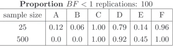
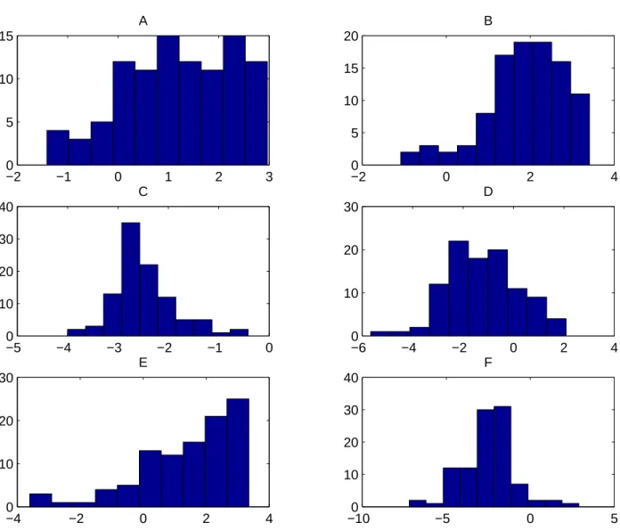
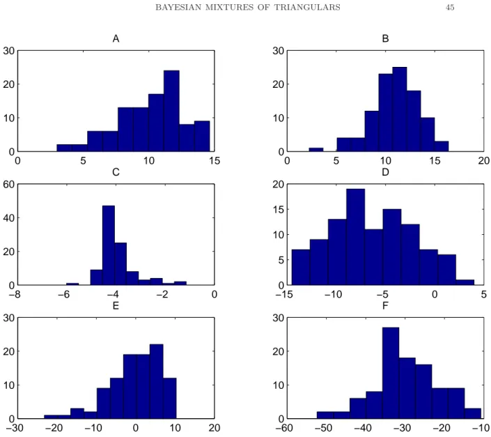
In all cases the parameters of the Beta distribution are assumed independent a priori with a Gamma distribution with parameters (3,0.5). A sample was generated from the posterior distribution using the Metropolis-Hastings algorithm and the marginal likelihood was computed from the output using the method described in Chib and Jeliazkov (2001). Sample sizes of n = 25 and n = 500 were used in the simulation study. The same densities (A)–(F) from section 2 are used. The results are summarized in the table below. Histograms of the Bayes factors are given in Figures 2 and 3.

Proportion BF < 1 replications: 100

sample size A B C D E F

25 0.12 0.06 1.00 0.79 0.14 0.96 500 0.0 0.0 1.00 0.92 0.45 1.00

The behaviour of the Bayes factor for these sample size is as predicted by the asymptotics with the possible exception of the truncated normal distribution. This density was included in the simulation study as it appears very close to a Beta density and so should be a challenging case for the Bayes factor.

Figure 2 near here. Figure 3 near here.

4.3. A distance approach. Now consider as in Robert and Rousseau (2004) the distance approach, based on the loss function:

L(δ, p) = (

a0d(p, Q) if δ = 0

a1(1 − d(p, Q)) if δ = 1

(4.1)

where δ = 0 corresponds to choosing the null hypothesis and δ = 1 corresponds to the alternative. The Bayes estimator is δ(Yn) = 0 if and only if

T (Yn) = Eπ[d(p, F)|Yn] ≤ a1/(a0+ a1) ,

and δ(Yn) = 1 otherwise. In a non informative set-up, where there is no prior information on how to calibrate (a0, a1), we use the Bayesian p-value pcpred defined

by pcpred(ˆθ, T ) = Z Θ Pθ h T (Xn_{) ≥ T |ˆ}θ, Ti_dπ(θ|ˆθ),

(27)

where ˆθ is the maximum likelihood estimator under the parametric family and as-sociated with the data (Yn) and

π0(θ|ˆθ) ∝ dπ(θ)pθ(Yn).

In this Section we prove that under the assumptions of Theorems 2.6 or 2.9, and if the parametric family is smooth enough, we have:

sup p0∈G(β),d(p0,Q)≥Cn−β/(2β+1) E₀nhpcpred(ˆθ, T ) i = O(n−1/2), (4.2)

where G(β) is the subclass of H¨older functions with regularity β, satisfying the as-sumptions of Theorems 2.6 or 2.9, and if p0 ∈ Q, pcpred(ˆθ, T ) = U(0, 1) + OP(n−1/2).

This implies that the test procedure is asymptotically optimal.

The result under the null hypothesis comes from Robert and Rousseau (2004). We therefore only have to study the behaviour of this test procedure under the alternative hypothesis.

Let θ⊥ _{= inf}

θ∈ΘR p0(x) log p0/pθ(x)dx, then the result of Robert and Rousseau

(2004) implies that

pcpred(ˆθ, T ) = Pθ⊥

h

T (Xn_{) ≥ T |ˆ}θ, Ti+ Rn,

where Rn goes to zero in probability. More precisely,

P₀n£_|Rn| > M log nt/√n¤≤ P0n

h

P_θ⊥[Ac_n|ˆθ] > M log nt/√n

i

+ O(n−1/2), where An is a set on which the Laplace approximation is valid. Under moment

conditions on the derivatives of the log-likelihood, it is well known that P_θ⊥[Ac_n] = O(n−H),

with H large enough (depending on the number of moments of the second and third derivatives of the log-likelihood).

Assume first that h(p0, pθ⊥) ≤ h0log n−2, where h(p, p′) denotes the Hellinger

distance between p and p′_{. Then using Lemma 6.2 in Appendix 6, we obtain that}

P0

h

P_θ⊥[Ac_n|ˆθ]

i

≤ Pθ⊥[Ac_n] + O(n−H) = O(n−H).

We therefore need only consider the quantity p_θ⊥_,n = P_θ⊥

h

(28)

From the inequality T (Yn_{) ≥ d(p}0, F) − Eπ[d(p0, p)|Yn], we obtain that P_θ⊥ h T (Xn_{) ≥ T |ˆ}θ, Ti _{≤ P}_θ⊥ h Eπ[d(p0, p)|Yn] + Eπ[d(pθ⊥, p)|Xn] ≥ d(p0, F)|ˆθ, Yn i . Therefore, as soon as d(p0, Q) > O(n−β/(2β+1)log n2) this quantity is small.

In-deed, define vn = v0n−β/(2β+1)log n2, for some constant v0 large enough, which

corresponds to the rate of convergence of Eπ_{[d(p, q)|Y}n_{] to zero (as obtained in}

E_θ⊥ h P_θ⊥ ³ Eπ[d(p_θ⊥, p)|Xn] ≥ d(p0, Q) − vn|ˆθ ´i ≤ n−H

for any H, as soon as d(p0, Q) ≥ 2vn. Using Lemma 6.2 in Appendix 6, we have

that E0 h P_θ⊥ ³ Eπhd(p⊥_θ_{, p)|X}ni_{≥ d(p}0, F) − vn(p0)|ˆθ ´i ≤ Eθ⊥ h P_θ⊥ ³ Eπhd(p⊥_θ_{, p)|X}ni´i+ O(n−1/2) ≤ O(n−1/2).

Finally, as soon as 2vn ≤ d(p0, Q) and h(p0, pθ⊥) ≤ c0log n−2, equation (4.2) is

proved under the above constraint.

If h(p0, pθ⊥) ≥ c₀log n−2, then d(p₀, Q) ≥ c₀log n−2. Using

E₀n[pcpred] = Z Θ π(θ)Pθ h T (Xn_{) ≥ T |ˆ}θ, Tidθ ≤ Z |θ−θ⊥_|<n−1/4 π(θ)Pθ h T (Xn_{) ≥ T |ˆ}θ, Tidθ + O(n−1), together with the fact that uniformly in θ, such that |θ − θ⊥| < n−1/4, we have

Pθ

£

(29)

which achieves the proof of equation (4.2).

This proves that the test procedure using pcpred and the statistic T (Yn) has an

optimal rate of convergence and good behaviour under the null hypothesis asymp-totically. The interest in such a procedure is that if a priori one is able to determine a1/(a0+ a1), which appears in the loss function, there is no need to use the

condi-tional predictive p-value and the test procedure has non-asymptotic properties such as admissibility. However if this a priori knowledge is not available, one can always the p-value pcpred as described above and the test procedure has good asymptotic

properties. Note that if the parametric family that is being tested belongs to the class of exponential families then under the null hypothesis the p-value is exactly uniform and the test procedure has good non-asymptotic properties.

5. Discussion

This paper has examined the asymptotic properties of Bayesian density estimates using a mixture of triangular prior. It was seen that the density estimates, under certain conditions, possess the desirable properties of weak and strong consistency. Both Type I and Type II mixture priors were seen to attain the minmax rate of convergence (up to a log n term) for H¨older continuous density functions when the true density is bounded below. From the results in Perron and Mengersen (2001) we believe that the Type II mixtures are better suited to situations where weak convergence of the estimate is of greater interest. This may be the case when the true distribution is believed to possess some multifractal property; see Falconer (1997). To the best of our knowledge, general conditions for determining weak rates of convergence have not been previously determined.

While general conditions for good priors have been established in Section 2 of this paper we have not discussed specific prior choice. Viewing the mixture of triangulars as a parametrization of a piecewise linear density function enables us to clearly see

(30)

the role of the prior distribution. In a Type I mixture the density can be seen to be the linear interpolation of the point (0, 2kw0) , {(xi, wik)}k−1i=1 (1, 2kwk) and hence

the role of w is clear. For computational simplicity a Dirichlet prior could be used with the parameters chosen to reflect an a priori belief on the shape of the density. Alternatively, the prior on w could be chosen to reflect a strong belief about other features of the density such as monotonicity or unimodality. A similar statement is possible for the Type II mixture of triangular distributions.

Sections 3 and 4 were devoted to the application of these prior distributions to goodness-of-fit testing. We have shown that Bayes factor will be consistent under very general conditions when testing a point null hypothesis. The case of a simple null hypothesis has received a detailed theoretical treatment in the literature, for example Verdinelli and Wasserman (1998) and Fortiana and Gran´e (2003). However, in practice a test against a parametric family with unknown parameters is required. We have been able to give sufficient conditions for consistency of the Bayes factor in this case and determined a rate of convergence under the null. Importantly situations in which the Bayes factor is inconsistent were identified. The inconsistency in the Bayes factor can arise if the nonparametric prior places too much probability near the true density relative to the parametric prior. For this reason, among others, a distance based approach was considered for the goodness-of-fit test. The distance approach produces a p−value which is asymptotically uniformly distributed under the null hypothesis and converges to zero under the alternative. Rates of convergence were also established. As the test statistic is based on the distance between densities the procedure is less sensitive to the prior than the Bayes factor. In particular, the distance approach is able to avoid the inconsistency that occurs with the Bayes factor.

6. Appendix 6.1. Appendix 1: Lemma 6.1.

Lemma 6.1. Let p_ψ(k)and p_η(k)be two type II mixtures of triangular densities where ψ(k) = (x0, x1, . . . , x_k−1, xk) and η(k) = (x0, ˜x1, . . . , ˜x_k−1, xk). For 0 < ǫ < 1/4, if

max

i |xi− ˜xi| ≤

ǫ

(31)

then sup x∈[0,1] ¯ ¯pψ(k)(x) − pη(k)(x) ¯ ¯ ≤ CMǫ, where C is a constant independent of the partitions and k.

Proof. This is a tedious calculation, hence its relegation to an appendix. Suppose that ˜xi = xifor all i 6= j and ˜xj < xj . As we have seen in the proof of Theorem 2.7

1

M k < |xi− xi−1| < 1 ak,

so under the assumptions of this lemma ˜xj ∈ [xj−1, xj+1]. If the partitions forming

p_ψ(k)and p_η(k)differ only at xj then the two densities will differ only on the interval

[x_j−2, xj+2]. We now calculate the difference between the component triangular

den-sities which form p_ψ(k), p_η(k) on [x_j−2, xj+2]. The triangular density on [xj−1, xj+1]

with mode at xj is ∆j(x) = ( ₂ (xj+1−xj−1) (x−xj−1) (xj−xj−1) x ∈ [xj−1, xj] 2 (xj+1−xj−1) (xj+1−x) (xj+1−xj) x ∈ [xj, xj+1]

and the triangular density on [x_j−1, xj+1] with mode ˜xj is

e ∆j(x) = ( ₂ (xj+1−xj−1) (x−xj−1) (˜xj−xj−1) x ∈ [xj−1, ˜xj] 2 (xj+1−xj−1) (xj+1−x) (xj+1−˜xj) x ∈ [˜xj, xj+1] . The greatest difference between these two densities occur at xj and ˜xj.

¯ ¯ ¯∆j(xj) − e∆j(xj) ¯ ¯ ¯ = _(x 2 j+1− xj−1) ¯ ¯ ¯ ¯1 − (xj− xj−1) (˜xj− xj−1) ¯ ¯ ¯ ¯ = 2|˜xj− xj| (xj+1− xj−1)(˜xj− xj−1) ¯ ¯ ¯∆j(˜xj) − e∆j(˜xj) ¯ ¯ ¯ = _(x 2 j+1− xj−1) ¯ ¯ ¯ ¯ (xj+1− ˜xj) (xj+1− xj)− 1 ¯ ¯ ¯ ¯ = 2|˜xj− xj| (xj+1− xj−1)(xj+1− xj)

Now consider the triangular densities on [xj, xj+2] and [˜xj, xj+2] with mode at xj+1.

∆j+1(x) = ( ₂ (xj+2−xj) (x−xj) (xj+1−xj) x ∈ [xj, xj+1] 2 (xj+2−xj) (xj+2−x) (xj+2−xj+1) x ∈ [xj+1, xj+2] and e ∆j+1(x) = ( ₂ (xj+2−˜xj) (x−˜xj) (xj+1−˜xj) x ∈ [˜xj, xj+1] 2 (xj+2−˜xj) (xj+2−x) (xj+2−˜xj) x ∈ [xj+1, xj+2]

(32)

The greatest difference between these two densities occur at xj+1 and ˜xj. ¯ ¯ ¯∆j+1(xj+1) − e∆j+1(xj+1) ¯ ¯ ¯ = 2 ¯ ¯ ¯ ¯ 1 (xj+2− xj) − 1 (xj+2− ˜xj) ¯ ¯ ¯ ¯ = 2|˜xj− xj| (xj+2− xj)(xj+2− ˜xj) ¯ ¯ ¯∆j+1(˜xj) − e∆j+1(˜xj) ¯ ¯ ¯ = _(x 2|˜xj− xj| j+2− xj)(xj+1− xj)

Similar calculations show that the difference between the two triangular densities on [x_j−2, xj] and [xj−2, ˜xj] with modes at xj−1 is greatest at xj and xj−1 giving

¯ ¯ ¯∆j−1(xj) − e∆j−1(xj) ¯ ¯ ¯ = _(˜_x 2|˜xj − xj| j− xj−2)(˜xj− xj−1) ¯ ¯ ¯∆j−1(xj−1) − e∆j−1(xj−1) ¯ ¯ ¯ = _(x 2|˜xj − xj| j− xj−2)(˜xj− xj−2)

Combining these bounds give sup x∈[0,1] ¯ ¯pψ(k)(x) − pη(k)(x) ¯ ¯ < 19 3 M 2 k |˜xj− xj| .

Now define ηj(k) = (x0, ˜x1, . . . , ˜xj, xj, . . . , xk−1, xk) , j = 1, . . . , k − 1. As each

triangular density shares support with at most two others, the two densities pηj−1, pηj

will differ only on the interval [˜x_j−2, xj+2]. Under the assumptions of the lemma is

easily seen that sup_xp_η_j_(k)(x) < 4₃_{M for all j = 1, . . . , k − 1. Hence,}

sup x∈[0,1] ¯ ¯ ¯pηj(k)(x) − pηj−1(k)(x) ¯ ¯ ¯ < 19₃ × µ 4 3 ¶2 M2_{k |˜x}j− xj| .

As the intervals [˜x_j−2, xj+2] overlap only four times we have

sup

x∈[0,1]|pψ(x) − pη(x)| ≤ CM

2_{k max}

i |˜xi− xi| ≤ CMǫ.

This completes the proof.

¤

(33)

Proof. Let p(.; w, k) be such that |1 − p(.; w, k)|1 ≤ √ρn and denote w′_j = wj for 1 ≤ j ≤ k − 1 and w′0= 2w0, wk′ = 2wk, then |1 − p(.; w, k)|1 = k−2 X j=1 Z (j+1)/k j/k ¯ ¯w′ j+1k2(x − j/k) + w′jk2((j + 1)/k − x) − 1 ¯ ¯ dx = k−1 X j=0 Z (j+1)/k j/k |aj + bjx| dx

where aj = k[wj′(j + 1) − w′j+1j] − 1 and bj = k2(w′j+1− w′j). Let ¯xj = −aj/bj =

j/k − w′j/k(wj+1′ − w′j) + 1/k2(w′j+1− w′j), • If j/k < ¯xj < (j + 1)/k then ∆j = Z (j+1)/k j/k |aj + bjx| dx = ¯ ¯ ¯ ¯aj(2¯xj− 2j/k − 1/k) + bj 2 ¡ 2¯x2_j_{− 2j}2/k2_{− 1/k}2_{− 2j/k}2¢ ¯ ¯ ¯ ¯ = |bj| ¯ ¯ ¯ ¯−¯x2j+ (2j + 1)¯xj k − j2 k2 − 1 2k2 − j k2 ¯ ¯ ¯ ¯ = |bj| ¯ ¯ ¯ ¯ ¯− µ ¯ xj −2j + 1 2k ¶2 −_4k12 ¯ ¯ ¯ ¯ ¯ = |bj| Ãµ ¯ xj − 2j + 1 2k ¶2 + 1 4k2 ! ≥ |w ′ j+1− wj′| 4 ≥ |w ′ j+1− 1/k| + |w′j− 1/k| 8 ,

since in this case we have either w′

j < 1/k < wj+1′ or w′j > 1/k > w′j+1. • If ¯xj ∈ (j/k, (j + 1)/k),/ ∆j = ¯ ¯ ¯ ¯ ¯ Z (j+1)/k j/k aj+ bjxdx ¯ ¯ ¯ ¯ ¯ = ¯ ¯ ¯ ¯[wj′(j + 1) − wj+1′ j] − 1 k + (wj+1− wj) 2 [1 + 2j] ¯ ¯ ¯ ¯ = ¯ ¯ ¯ ¯w′j− 1 k + (w′_j+1_{− w}_j′) 2 ¯ ¯ ¯ ¯ ≥ |w ′ j− 1/k| 2

(34)

The latter inequality comes from the fact that when ¯xj ∈ (j/k, (j + 1)/k),/

then we have either w′_j+1> w_j′ > 1/k or w_j+1′ < w_j′ < 1/k.

Finally we obtain the result of Lemma 3.4 ¤

6.3. Appendix 3: Proof of Lemma 3.5.

Proof. We consider the same type of calculations as in the case of type I mixtures. ∆j =

Z xj+1

xj

|aj+ bjx| dx

but this time aj = −2 · pj+1xj Dj+1 − pjxj+1 Dj ¸ 1 xj+1− xj − 1, bj = 2 · pj+1 Dj+1 − pj Dj ¸ 1 xj+1− xj

where Dj = xj+1− xj−1 for 1 ≤ j ≤ k − 1, D0 = x1 and Dk= (1 − xk−1). We still

have ¯xj = −aj/bj and the following two conditions ¯xj ∈ (xj, xj+1) or ¯xj ∈ (x/ j, xj+1)

• If ¯xj ∈ (xj, xj+1). ∆j = ¯ ¯ ¯ ¯aj(2¯xj− xj− xj+1) + bj 2 ¡ 2¯x2_j _{− x}2_j _{− x}2_j+1¢ ¯ ¯ ¯ ¯ = |bj|¡(¯xj− (xj + xj+1)/2)2+ (xj− xj+1)2¢. If k > j ≥ 1 ∆j = ¡(¯xj − (xj+ xj+1)/2)2+ (xj− xj+1)2¢ 2 k ¯ ¯ ¯D−1j+1− Dj−1 ¯ ¯ ¯ (xj+1− xj)−1 ≥ 2(xj+1_k− xj)¯¯¯Dj+1−1 − D−1j ¯ ¯ ¯ .

and Moreover ¯xj ∈ (xj, xj+1) if and only if Dj∧ Dj+1< 2/k < Dj∨ Dj+1,

so that ∆j ≥ 2(xj+1− xj) k ¯ ¯ ¯Dj+1−1 − k/2 ¯ ¯ ¯ + ¯ ¯ ¯Dj−1− k/2 ¯ ¯ ¯ . • If ¯xj ∈ (x/ j, xj+1), ∆j = ¯ ¯ ¯ ¯aj(xj+1− xj) + bj 2 ¡ x2_j+1_{− x}2_j¢ ¯ ¯ ¯ ¯ = (xj+1− xj) k ¯ ¯ ¯ ¯ 1 Dj+1 + 1 Dj − k ¯ ¯ ¯ ¯ ≥ (xj+1_k− xj)µ¯¯¯_¯_D1 j+1 − k 2 ¯ ¯ ¯ ¯ + ¯ ¯ ¯ ¯ 1 Dj − k 2 ¯ ¯ ¯ ¯ ¶ .

(35)

We now consider ∆0 and ∆k. Similar calculations imply that ∆0 ≥ 1 2kx2 |x1− x2/2| , ∆1 ≥ 1 2k(1 − xk−2)|(1 − xk−1) − (1 − xk−2)/2|

We finally obtain that |1 − fk|1 ≥ k−1 X j=1 (xj+1− xj) 2k µ¯¯_¯ ¯ 1 Dj+1 − k 2 ¯ ¯ ¯ ¯ + ¯ ¯ ¯ ¯ 1 Dj − k 2 ¯ ¯ ¯ ¯ ¶ + 1 2kx2 |x1− x2/2| + 1 2k(1 − xk−2)|(1 − xk−1) − (1 − xk−2)/2|

and Lemma 3.5 is proved. ¤

6.4. Appendix 4: Proof of Lemma 3.6. Let ρn = ρ0log n2p/n. We consider

tests as defined in Ghosal et al. (2000) based on the L1 distance: We know that

there exists tests φi associated with densities pi∈ Vnc such that

E₀n[φi] ≤ e−nK|1−pi| 2 sup p:|p−pi|≤|1−pi|/5 E_fn_{[(1 − φ}i)] ≤ e−nK|1−pi| 2 .

Consider Fn= {pξ(k), k ≤ kn, ξ(k) : sup_x∈[0,1]pξ(k)(x) ≤ na} where kn= k0log np−1,

with p ≥ 2. Following Lemma 6.1 we have that the number of balls required to re-cover the set Fn∩ Vnc is bounded by

Dn= kn µ cknn2a ρn ¶kn ≤ ek0(2a+1) log np

so that, by considering k0 small enough we have that if φn= maxiφi

E₀n(φn) ≤ ek0log n p_(2a+1) e−Kρ20log np ≤ e−c log np Therefore, if I21= Z Vc n∩Fn pη(Yn)dπ(η), we obtain that P₀n£I21≥ vn−1 ¤ ≤ E0n[φn] + E0n h (1 − φn)1I_(I₂₁_≥v−1 n ) i ≤ E0n[φn] + vn Z Vc n∩Fn E_p(ξ)_{(1 − φ}n)dπ(ξ) ≤ E0n[φn] + vnπ (Vnc∩ Fn) e−K log n p ≤ n−H

(36)

for any positive H, when n is large enough. We finally consider I22= Z Fc n pη(Yn)dπ(ξ); and P₀n£I22≥ v−1n ¤ ≤ vnπ(Fnc) ≤ vnπ[k ≥ k0log np−1] + O(n−H) ≤ O(n−H) for any H > 0 .

6.5. Appendix 5: Proof of lemma 4.2. We are trying to give a lower bound on the L1 norm between the mixture of triangular densities and p0. If we can show

that (6.1)

Z 1 0 |p

0(x) − pk(x)| dx ≥ ck−α

where pk is the mixture of triangular densities with k components that best

ap-proximates p0 in the L1 distance and c, α are constants, then from the discussion

following Theorem 2.6 the prior probability on Aǫn will be bounded by

for any κ < β/((2β + 2)α). Hence, nd/2_{π (A}

ǫn) −→ 0 for any finite d provided we

can show that α < ∞.

From the assumptions of lemma, for all k sufficiently large there exists a j such that [j/k, (j + 1)/k] ⊂ I. It will be assumed that the second derivative is negative on I, the proof will follow the same arguments if it is positive. We proceed now to find a lower bound on the L1 norm.

(37)

where a and b are chosen to minimize the integral. As p0 is strictly concave on the

interval [j/k, (j + 1)/k] the line a + bx will intersect p0 at two points x1, x2. The

line joining (x1, p0(x1)) and

¡_x₁_+x₂ 2 , p0 ¡_x₁_+x₂ 2 ¢¢ is l1(x) = Ã p0¡x1+x₂ 2¢− p0(x1) x2− x1 ! 2 (x − x1) + p0(x1) , and satisfies l1(x) < p0(x) , x ∈ µ x1, x1+ x2 2 ¶ . Similarly, the line joining¡x1+x2

2 , p0 ¡_x₁_+x₂ 2 ¢¢ and (x2, p0(x2)) is l2(x) = Ã p0(x2) − p0 ¡_x₁_+x₂ 2 ¢ x2− x1 ! 2 (x − x2) + p0(x2) , and satisfies l2(x) < p0(x) , x ∈ µ x1+ x2 2 , x2 ¶ .

The L1norm between p0and pkis bounded below by the area of the triangle formed

by (x1, p0(x1)) ,¡x1+x₂ 2, p0¡x1+x₂ 2¢¢and (x2, p0(x2)). From basic geometry this area

is _· p0 µ x1+ x2 2 ¶ −p0(x1) + p₂ 0(x2) ¸ µ x2− x1 2 ¶

Taking a Taylor expansions of p0;

p0 µ x1+ x2 2 ¶ −p0(x1) + p₂ 0(x2) = 1 2 µ x2− x1 2 ¶ · p′₀(x1) − p′0(x2) + µ x2− x1 2 ¶ µ p′′ 0(x1) 2 + p′′ 0(x2) 2 ¶ +O (x2− x1)2 i = 1 2 µ x2− x1 2 ¶2· −2p′′0(x2) + p′′ 0(x1) 2 + p′′ 0(x2) 2 + O (x2− x1) 2¸ = 1 2 µ x2− x1 2 ¶2_£ −p′′0(x2) + O (x2− x1)¤ Hence, Z 1 0 |p0(x) − pk(x)| dx > 1 2 µ x2− x1 2 ¶3_£ −p′′0(x2) + O (x2− x1) ¤

and assuming (x2− x1) > k−2 then

Z 1

0 |p0(x) − pk(x)| dx > Ck −6

(38)

for some constant C, as required.

Now suppose that |x2− x1| ≤ k−2. For ease of notation assume that j = 0.

Consider the tangent line at x = 0 given by

t (x) = p0(0) + p′0(0) x.

As p0 is strictly concave on the interval [j/k, (j + 1)/k] it satisfies

t (x) > p0(x) , x ∈ (0, 1/k) .

The line joining the points (x1, p0(x1)) and (x2, p0(x2)) is given by

l3(x) =

p0(x2) − p0(x1)

x2− x1 (x − x1

) + p0(x1) ,

which is the line which minimizes the L1 norm on the interval [j/k, (j + 1)/k]. The

point of intersection between t (x) and l3(x) is

x∗ = p0(x1) − x1 p0(x2)−p0(x1) x2−x1 − p0(0) p′₀_{(0) −} p0(x2)−p0(x2) x2−x1 = p0(x1) − p0(0) − x1(p′0(x1) + O (x2− x1)) p′₀_{(0) − p}′₀(x1) + O (x2− x1) = x1 p′′₀(x1) p′′ 0(0) + O¡x2₁¢+ O (x2− x1) ,

provided (x2− x1) ≤ k−2 and x1 > k−3/2. The area of the triangle formed by

(0, t (0)) , (x∗, t (x∗)) and (0, l3(0)) is x∗ 2 |l3(0) − t (0)| = x∗ 2 ¯ ¯ ¯ ¯p0(x1) − x1p0(x2) − p0(x1) x2− x1 − p0 (0) ¯ ¯ ¯ ¯ = x∗ 2 ¯ ¯p0(x1) − p′0(x1) x1− p0(0) + O (x1(x2− x1)) ¯ ¯ = x∗ 2 ¯ ¯ ¯ ¯− x2 1 2 p ′′ 0(x1) + O (x1(x2− x1)) + O¡x31 ¢¯¯ ¯ ¯ = − (p′′0(x1)) 2 2p′′₀(0) x 3 1+ O ¡ k−5¢ Thus, Z 1 0 |p0(x) − pk(x)| dx > Ck −4.5

if x1> k−3/2and x2− x1 ≤ k−2. For the final case of x1≤ k−3/2and x2− x1 ≤ k−2