Are risk averse agents more optimistic? A Bayesian estimation
approach
Selima Ben Mansour, Elyès Jouiniyz, Jean-Michel Marinx, Clotilde Napp* and Christian Roberty June 15, 2007
Abstract
Our aim is to analyze the link between optimism and risk aversion in a subjective ex-pected utility setting and to estimate the average level of optimism when weighted by risk tolerance. This quantity is of particular importance since it characterizes the consensus be-lief in risk-taking situations with heterogeneous bebe-liefs. Its estimation leads to a nontrivial statistical problem. We start from a large lottery survey (1,536 individuals). We assume that individuals have true unobservable characteristics and that their answers in the survey are noisy realizations of these characteristics. We adopt a Bayesian approach for the statistical analysis of this problem and use an hybrid MCMC approximation method to numerically estimate the distributions of the unobservable characteristics. We obtain that individuals are on average pessimistic and that pessimism and risk tolerance are positively correlated. As a consequence, we conclude that the consensus belief is biased towards pessimism.
Keywords: Bayesian estimation, MCMC scheme, importance sampling, pessimism, risk tolerance, risk aversion, consensus belief.
1
Introduction
Optimism is usually conceived as a personal trait leading to overestimate the likelihood of good outcomes and to underestimate the likelihood of bad outcomes. Previous work related to this issue includes psychological surveys as well as empirical studies on professionals’economic forecasts (see, e.g., Fried and Givoly, 1982, O’Brien, 1988, Francis and Philbrick, 1993, Kang et al., 1994, Dreman and Berry, 1995, Giordani and Söderlind, 2005).
Risk aversion in decision making intuitively corresponds to the fact that when facing choices with comparable returns, agents tend to choose the less risky alternative. This feature has been largely studied in particular in relation with other personal characteristics like gender, age, income, education (see, among others, Binswanger, 1980, 1981, Palsson, 1996, Barsky et al., 1997, Eisenhauer and Halek, 2001, Eisenhauer and Ventura, 2003, Felton et al., 2003, Guiso and Paiella, 2001).
In the setting of a Subjective Expected Utility (SEU) model, risk aversion is measured by the curvature of the utility function and optimism is characterized by the individual subjective probability. Risk aversion and individual subjective probability completely determine the indi-vidual decision-making behavior, at least locally. The SEU model is particularly well adapted to the aggregation problem and recent papers show how individual risk aversions and subjective probabilities are aggregated at the collective level in such a setting (Calvet et al. 2002, Gollier, 2007, Jouini and Napp, 2006, 2007, Li, 2006).
DRM, UMR-CNRS 7088, Université Paris-Dauphine
yCEREMADE, UMR-CNRS 7534, Université Paris-Dauphine.
zCorresponding author: [email protected], phone: +33 1 44 05 42 26, fax: +33 1 44 05 48 49. xInria
From an empirical point of view, these two notions are hard to disentangle. For instance, in the context of lotteries, which is often used to measure the risk aversion level, the reservation price of a risk averse (resp. risk tolerant) and unbiased individual is empirically indistinguishable from the reservation price of a risk neutral and pessimistic (resp. optimistic) individual; there is here an identi…cation problem that confounds data interpretation.
In this paper, we start from a lottery survey, in which data on both risk aversion (reservation price) and subjective beliefs (subjective probabilities) is available in the same context. In the setting of a SEU model, this survey enables us to disentangle both notions and to infer about the individual levels of optimism and of risk aversion. Our aim is then to determine and to understand the nature of the link between optimism and risk aversion. More precisely, we
want to estimate the average level of optimism weighted by the risk tolerance1 as well as the
unweighted average.
The estimation of these quantities is important for both following reasons. First, since the di¤erence between the weighted average and the unweighted average of the individual level of optimism is precisely given by the covariance between risk tolerance and optimism, the estimation of these averages will give us the nature of the correlation between risk tolerance and optimism. The determination of this correlation should shed some light on the determinants of the level of optimism and/or risk aversion at the individual level. Second, the estimation of the weighted average of the individual beliefs is of particular importance at the collective level. Indeed, in the setting of collective risk-taking decisions with heterogeneous beliefs (and SEU), this average subjective belief represents the consensus of the group (see Gollier, 2007).
Analogously, in CCAPM2-like equilibrium models with heterogeneous beliefs (and SEU), the
weighted average of the individual beliefs3 represents the belief of the representative agent (see
Rubinstein, 1976, Detemple and Murthy, 1994, Calvet et al., 2002, Abel, 1989, Zapatero, 1998, Jouini and Napp, 2006, 2007, Li, 2006). This consensus belief plays a crucial role on the Pareto optimal risk sharing rules and on the equilibrium properties. In particular, a pessimistic
consensus belief might help in explaining the risk premium and risk free rate puzzles4.
We analyze answers to a large survey (1536 individuals). The main problem we encounter in this survey is related to the fact that some observations correspond to risk neutral or even risk seeking behaviour. Note that the presence of risk seeking or risk neutral individuals in the panel is not surprising. Similar results have been obtained in the literature (Guiso and Paiella, 2001, Eisenhauer and Ventura, 2003, Hartog et al., 2002). However, these observations are not compatible with the standard assumptions of decision theory and of CCAPM-like equilibrium models nor with the existence of an equilibrium with positive risk-premia since at such an equilibrium, agents are, at least locally, risk averse. Since our aim is to estimate the risk tolerance weighted average of the individual levels of optimism at the equilibrium, these observations require a speci…c analysis. It is not possible to simply reject these observations, since they are associated with high levels of risk tolerance and their rejection would have a strong impact on the quantities to be estimated. We can not keep them without a speci…c treatment since, for these individuals, the risk tolerance level is in…nite or negative, and with such in…nite or negative weights, an average weighted by the risk tolerance becomes meaningless. We propose then to interpret both risk neutrality and risk seeking as noise and we adopt the following approach; we assume that individuals have true unobservable characteristics that respect the assumptions of decision theory, and we interpret the answers in the survey as noisy realizations of those characteristics. This is not an original treatment of the data and it is in the spirit of the Quantal Response Equilibrium model of McKelvey and Palfrey (1992) where it is assumed, in a game theoretic framework, that with some probability, and for reasons that are completely
1Risk tolerance is de…ned as the inverse of risk aversion. 2
Consumption-based Capital Asset Pricing Model.
3When agents are assumed to have log utilities, this corresponds to the wealth weighted average belief. 4
As shown by Mehra and Prescott (1985) and Weil (1989), standard models of …nancial markets equilibrium predict risk-premia (resp. risk-free rates) that are too low (resp. too high) to …t observed data.
orthogonal to the model, a player might choose actions that are not in accordance with the predictions of the model: agents do not select systematically their best-responses, but they play these strategies with a higher frequency. This approach has been shown to be powerful to organize behavior in numerous experimental settings.
The aim is then to estimate the distribution of the unobservable characteristics and to derive the value of the average level of optimism weighted by the risk tolerance. We follow a Bayesian approach for this purpose and use an MCMC approximation method for computational reasons. We emphasize that we do not pretend to compute a precise level of optimism of the consensus belief in a general setting but rather to determine whether there is a clear spread between the weighted and unweighted averages, which would indicate a behavioral correlation between optimism and risk aversion and a pessimistic bias at the collective level.
The paper is organized as follows. Section 2 presents the data as well as the measures of individual optimism and risk aversion. Section 3 presents the statistical estimation. Section 4 concludes.
2
The data
We …rst describe the survey, then we present the adopted risk aversion and optimism measures. The last subsection deals with data consistency results.
2.1 The survey instrument
We start from answers to a survey conducted face-to-face in the …eld by professional interviewers. The sample is made of adults, between 22 and 55, that are randomly chosen, and yielded 1,536
responses. The questionnaire consists of essentially …ve parts5.
In the …rst part, the participant is asked about his reluctance to take part in a game of chance for religious grounds. Only those who do not have such interdict go on with the questionnaire. In the second part, the participant is o¤ered the opportunity of entering a head and tail game for ten rounds. More precisely, a coin is being ‡ipped ten times; each time head occurs, the participant is supposed to get 10 Euros. The participant is then asked for his own estimation of the number of times head will occur. The participant is also asked to reveal the maximum amount he is willing to pay in order to take part in this game. The aim of this second part is to obtain, in the same setting, measures of the individual levels of optimism and of risk aversion.
The third part deals with questions similar to those in Barsky et al. (1997) which lead to the elicitation of the level of individual relative risk aversion. This part will enable us to verify that the data on absolute risk aversion is consistent with the data on relative risk aversion at the individual level. The fourth part deals with optimism questions as in Wenglert and Rosen (2000) while the …fth part deals with personal questions, such as gender, age, marital status, employment status, education and income.
These last three parts will make it possible to compare the results obtained on our sample with those usually obtained in the literature in terms of Risk aversion, optimism and their determinants.
2.2 Risk aversion and optimism measures
We derive individual measures of risk aversion and of optimism from the answers to the survey. As in Ben Mansour et al. (2006), we derive a measure of the degree of optimism from the answers to the …rst question of the second part of the questionnaire "Imagine that a coin will be ‡ipped 10 times. Each time, if head, you win 10e. What is your own estimation, according to your experience and your luck, of the number of times head will occur, i.e. how many times
5
(out of ten) do you think you are going to win (and get 10e)?" This measure of optimism6 is
directly given by the number of times xi that the individual i thinks he is going to win. An
optimistic individual is characterized by a value of xi above the objective value of 5 and the
distance to 5 measures the intensity of his optimism.
This measure is obviously compatible with the de…nition of optimism as a transformation of the objective distribution into a more favorable one. Indeed, the subjective probability of
individual i associated to the favourable event “head occurs” is approximated by i = 10xi and
an optimistic individual is characterized by a i strictly higher than 0:5. We will use this
measure of individual subjective probability when determining a measure of risk aversion in the framework of Subjective Expected Utility. Notice that the introduction of a ten times head-tail game is intended to provide the individuals with a simple framework, helping them to reveal their subjective probability associated with the event “head occurs”.
As far as risk aversion is concerned, we recall that absolute risk aversion is de…ned by the
quantity A (c) = uu000(c)(c); whereas relative risk aversion is de…ned by R (c) = c
u00(c)
u0(c); where u
denotes the agent’s utility function. Adopting an approach similar to Guiso and Paiella (2001), we will use the answers to the question "What is the maximum amount that you are willing to pay to take part in the game?" to derive a measure of the individual level of absolute risk
aversion. The answer of individual i, denoted by yi; corresponds to his reservation price, which
leaves him indi¤erent between his initial wealth and the expected gain from the game. This
means that if we adopt the SEU model and if we let eX denote the random payo¤ associated
with the head-tail game, the answer yi satis…es
ui(wi) = Ei h ui wi+ eX yi i = 10 X k=0 C10k ki (1 i)10 kui(wi+ 10k yi) ;
where ui denotes the utility function of agent i, wi his initial wealth and Ei the expectation
operator under his subjective probability. In the case of exponential utility functions7, a measure
for (corrected) absolute risk aversion of individual i is then given by the nonzero solution ai of
1 =
10
X
k=0
C10k ki (1 i)10 kexp ai(yi 10k) :
It is easy to obtain through a simple factorization that this equation is equivalent to
1 = iexp ai
yi
10 10 + (1 i) exp ai
yi
10: (1)
We denote by CAi the nonzero solution, obtained by numerical approximation, of Equation (1).
We refer to it as Corrected absolute risk Aversion because we take into account the subjective
probability iin order to determine the individual level of risk aversion. For example, a pessimist
who believes = 3 and chooses y = 10 has an absolute risk aversion of a = 0:35; whereas an
optimist who believes = 3 and yet chooses y = 10 has an absolute risk aversion of a = 1:2:
This approach is di¤erent from the classical approach in experimental or empirical literature on risk aversion in an expected utility framework, where the possibility of subjective beliefs is usually not taken into account. For instance, in Guiso and Paiella (2001), when the individual is told to have a chance of 1 over 10 of winning, one does not take into account, both in the interpretations of the results and in the inferred levels of risk aversion, the fact that some
6Ben Mansour et al. (2006) provide a rationale for this measure as well as an analysis of its main features. 7
The choice of exponential utility functions amounts to assuming constant absolute risk-aversion. It permits numerical computations of the level of absolute risk-aversion without information about the individual level of wealth.
people believe that they are lucky and overweight their probability of winning while others do the opposite. The same remark holds for empirical approaches. For instance, Eisenhauer and Halek (2001) estimate the level of risk aversion using life insurance data. The underlying model assumes an age based estimated probability of mortality, i.e. assumes that all people in the same age class share the same objective estimation of their probability of mortality, whereas it is intuitive that the estimation of one’s probability of mortality is subjective and highly dependent upon one’s optimism.
2.3 Consistency of the data
In this section we verify the consistency of our data from di¤erent points of view.
First, the answers of our sample seem consistent with previous surveys. As far as relative risk aversion is concerned, we …nd that women are more risk averse (as in Eisenhauer and Halek, 2001, Barsky et al., 1997, Cohn et al., 1975, Palsson, 1996, Jianakoplos and Bernasek, 1998, Hariharan et al., 2000) and that relative risk aversion increases with age (as in McInish, 1982, Morin and Suarez, 1983, Riley and Chow, 1992, Palsson, 1996, Schooley and Worden, 1996, Wang and Hanna, 1997, Barsky et al., 1997).
The answers about optimism in the fourth part are also consistent with previous surveys. We obtain on our sample the same results as Wenglert and Rosen (2000) about personal optimism. Indeed, Wenglert and Rosen (2000) obtain an average level of "personal optimism" equal to 0.596 and we obtain a value of 0.536 (using the same methodology).
The consistency with previous surveys is also con…rmed by the data on reservation prices.
Let us denote by OAi the nonzero solution of Equation (1) for i = 12; i.e. the nonzero solution
ai of 1 = 1 2exp ai yi 10 10 + 1 2exp ai yi 10:
In other words, OA corresponds to the absolute risk aversion under the objective probability as it is usually computed in the literature. We obtain that OA is higher for women, increases with age and decreases with income as in Guiso and Paiella (2001), Donkers et al. (2001), Hartog et al (2002), Powell and Ansic (1997), Eisenhauer and Ventura (2003).
A possible drawback of our approach is that we use essentially two simple questions only to elicit individual risk attitudes. In fact, the survey contains various questions that involve risk aversion or optimism. In order to elicit one of these characteristics, the classical procedure would be a regression based on all the questions related to that characteristic. However, our aim is to determine both characteristics in the same context in order to disentangle the two notions and to obtain a measure of risk aversion that is corrected by the level of optimism.
For this reason, we have chosen to determine a measure of the individual levels of optimism and risk aversion from the answers to the head and tail questions only and then to verify their consistency with the answers to other questions in the survey.
We verify that the answers about the reservation price are compatible with those about relative risk aversion. By de…nition, relative risk aversion is equal to the product of absolute risk aversion by individual wealth. We consider individual income as a proxy for individual wealth. Since the level of relative risk aversion derived from our survey is a qualitative variable (individuals are sorted into seven groups), we establish the consistency between relative and absolute risk aversion measures through a comonotonicity test between relative risk aversion and the product of absolute risk aversion by the mean of the income band (see Table 1).
Finally, as far as the data on the subjective probabilities are concerned, three questions in the questionnaire on personal pessimism have attracted our attention since intuitively, they should have a link with our notion of pessimism : (Q1) You have no chance to win at a lottery game, (Q2) You have no chance to be selected for a television game and (Q3) You will win one day at the Promosport. As expected, we have obtained a decreasing relationship between (Q1)
(resp. Q2) and our measure of optimism and an increasing relationship between (Q3) and our measure of optimism.
3
Statistical estimation
In this section we adopt a Bayesian approach (see, e.g., Robert, 2001) for the estimation of the average of the subjective probabilities weighted by the risk tolerance. We also estimate the unweighted average of the subjective probabilities.
The estimation of these quantities is interesting at the individual level, and can help to understand the nature of the link between risk aversion and optimism. Indeed, the correlation between risk aversion and optimism is easily deduced from the di¤erence between these two quantities.
Moreover, the estimation of the weighted and unweighted averages of the individual beliefs is of particular importance at the collective level. Indeed, in the setting of collective risk-taking decisions with heterogeneous beliefs (and SEU), this average subjective belief represents the consensus of the group. Analogously, in CCAPM-like equilibrium models with heterogeneous beliefs (and SEU), the weighted average of the individual beliefs represents the belief of the representative agent. The determination of the consensus belief, or more precisely of the extent to which it di¤ers from the unweighted average of the subjective beliefs, is then particularly interesting.
We do not pretend here to be able to compute precise and reliable individual and collective levels of risk aversion or of optimism. We are interested in observing whether there is a clear spread between the weighted and unweighted averages, which would indicate a behavioral cor-relation between optimism and risk aversion and a pessimistic bias at the collective level. In particular, it is well-known that willingness-to-pay questions are biased but this bias should not induce by itself a correlation between optimism and risk aversion.
3.1 Descriptive statistics
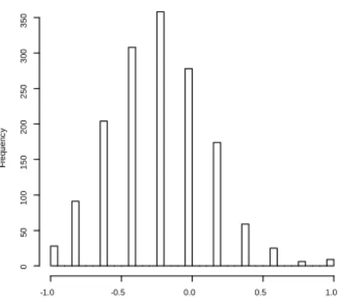
The results on the measure of optimism introduced in Section 2 have been studied in Ben Mansour et al. (2006). We recall here the main features of this analysis. Figure 1 provides the distribution of our measure of optimism among individuals and shows that there is a great heterogeneity in the level of optimism among agents. For the considered sample of 1,536 in-dividuals, the mean value for the number of times the individual thinks he is going to win is equal to 3.93. It is signi…cant and quite striking to observe that when asked about the number of times he is going to win at a head and tail game for ten draws, an average individual does not answer 5 times as he should if thinking under the objective probability, but answers slightly less than 4 times. This result is in favor of the existence of a behavioral bias towards pessimism in individual beliefs.
Regarding risk aversion, the average announced price is 11.96e which, as expected, is lower than the average subjectively expected payo¤. However some agents announced a reservation price higher than their subjectively expected gain hence have a negative corrected risk aversion.
This can be shown if we focus on the probabilities and prices that we denoted respectively by xi
and yi and if we represent them on a diagram. Figure 2 contains a jitter8 representation of this
diagram. There are 55 points such that y=100 = x=10 and 40 points such that y=100 > x=10. Based on Figure 2, it appears that there is a negative link between non corrected risk aversion and optimism, leading us to conclude that risk aversion (in the usual sense) decreases with optimism. Indeed, the average announced price for a given level of optimism clearly increases with the level of optimism. This correlation is con…rmed as statistically signi…cant by 8The jitter representation is used to improve the rendering on samples on grids by introducing a slight
Pearson, Kendall and Spearman tests. This is clearly understandable since the more optimistic an individual, the lower his non-corrected risk aversion. In other words, the non-corrected measure of risk aversion contents a great dose of pessimism. This negative correlation does not hold for corrected risk aversion. On the contrary, we veri…ed through Spearman’s and Kendall’s tests that the average of the corrected risk aversion for a given level of optimism signi…cantly increases with the level of optimism (see Table 2). This is in favor of a positive correlation between risk aversion (in our sense) and optimism.
3.2 The Bayesian model
We now want to estimate the average level of optimism weighted by the risk tolerance. The problem is that there is a non negligible number of individuals for which y=100 = x=10 (i.e. zero corrected risk aversion and in…nite corrected risk tolerance) or even y=100 > x=10 (i.e. negative corrected risk aversion and risk tolerance). The presence of such individuals raises some speci…c problems since with such negative or in…nite weights, the weighted sum is not a weighted average any longer. Furthermore, we can not simply eliminate these observations; indeed, the individuals for which y=100 is near x=10 are those for which the corrected risk tolerance level is high, hence they are heavily weighted in the considered average. Finally, such observations are incompatible with the classical assumptions of decision theory and CCAPM-like equilibrium models.
For all these reasons, a speci…c treatment of the data needs to be undertaken. One should bear in mind the fact that any slight modi…cation of an observation such that y=100 is near x=10 has a strong impact on the risk tolerance level and then on the weight in the considered average.
Note that the presence of risk seeking or risk neutral individuals in the panel is not surprising. Similar results have been obtained in the literature (Guiso and Paiella, 2001, Eisenhauer and Ventura, 2003, Hartog et al., 2002). However, our aim is to provide a proxy for the risk aversion at the equilibrium where at least locally, the agents are necessarily risk averse. For this reason, we propose to interpret both risk neutrality and risk seeking as resulting from noise.
More precisely, we adopt the following approach. We assume that individuals have true
un-observable characteristics ( i; pi); where i corresponds to the subjective probability of success
at each draw and pi corresponds to the price that the individual is willing to pay for the ten
draw game normalized to one (i.e. divided by 100). The answer (xi; yi) is then interpreted as a
noisy realization of ( i; pi).
More precisely, we assume that (x; y) = ((x1; y1); : : : ; (xn; yn)) is a set of independent
real-izations such that
(xi; yi) j( i; pi) B(10; i) B(100; pi);
where n is equal to 1536.
We now follow a Bayesian strategy to infer about the parameter ( i; pi), …rst de…ning a
prior distribution on this parameter as f( ;p)( i; pi) =
a 1
i (1 i)b 1pc 1i (1 pi)d 1( i pi)e
g(a; b; c; d; e) I0<pi< i<1 (2)
where a; b; c; d; e are positive constants and g(a; b; c; d; e) = B(a + c + e; b)B(c; e + 1) + 1 X i=1 ( d + 1) : : : ( d + i) i! B(a + c + e + i; b)B(c + i; e + 1):
We have then f ((x1; y1; 1; p1); : : : ; (xn; yn; n; pn)ja; b; c; d; e) = n Y i=1 Cxi 10 xi i (1 i) 10 xi If0;:::;10g(xi)C100yi piyi(1 pi)100 yiIf0;:::;100g(yi) a 1 i (1 i)b 1p c 1 i (1 pi)d 1( i pi)e g(a; b; c; d; e) I]0;1[( i)I]0; i[(pi)
which is a joint distribution on the data (x; y) and on the parameter. The Bayesian estimation is based on the so-called posterior distribution of the parameter, which simply is the conditional
distribution of this parameter given the data, f( ;p)( 1; p1; : : : ; n; pnjx; y; a; ; e).
The sample ( ; p) = (( 1; p1); : : : ; ( n; pn)) is not observed and, in addition, we …rst assume
that the so-called hyperparameters a; b; c; d; e are also unknown and thus need to be estimated from the data (x; y) (using similar Bayesian principles).
Once (a; b; c; d; e) is estimated, we want to estimate the average subjective probability weighted by the risk tolerance as well as the unweighted average subjective probability. For a given pair ( ; p); the associated level of risk aversion z( ; p) is de…ned as the solution in z of
exp(z(p 1)) + (1 ) exp(zp) 1 = 0
which is the analog of Equation (1). Hence, based on the data (x; y), we want to estimate the ratio E[ =z( ; p)]=E[1=z( ; p)]; which is given by
I = Z 1 0 Z u 0 u z(u; v) ua 1(1 u)b 1vc 1(1 v)d 1(u v)e g(a; b; c; d; e) dv du Z 1 0 Z u 0 1 z(u; v) ua 1(1 u)b 1vc 1(1 v)d 1(u v)e g(a; b; c; d; e) dv du = I3 I4 :
The natural Bayes estimate of this ratio is then the posterior expectation, E[I3=I4jx; y] (see
Robert, 2001, Chapter 2).
The unusual prior distribution for ( ; p) given in (2) is inspired from Beta distributions that
are the conjugates of binomial distributions, the additional term ( i pi)e being chosen for
integrability reasons. Indeed, near the diagonal, we have that z( ; p) p and thus the
nature of the integrals I3 and I4 depends on the position of e with respect to zero.
We will also estimate the unweighted average level of optimism I1 as well as the unweighted
average level of risk aversion I2, respectively given by
I1 = Z 1 0 Z u 0 ua(1 u)b 1vc 1(1 v)d 1(u v)e g(a; b; c; d; e) dv du Z 1 0 Z u 0 ua 1(1 u)b 1vc 1(1 v)d 1(u v)e g(a; b; c; d; e) dv du I2 = Z 1 0 Z u 0 z(u; v)u a 1(1 u)b 1vc 1(1 v)d 1(u v)e g(a; b; c; d; e) dv du Z 1 0 Z u 0 ua 1(1 u)b 1vc 1(1 v)d 1(u v)e g(a; b; c; d; e) dv du :
3.3 Parameter estimation and numerical results
To complete the de…nition of the prior distribution, we also introduce the following exponential prior on the hyperparameters:
Once the prior and the sampling distributions selected, we can formally draw inference about
the true parameters ( i; pi) by computing their posterior distribution, that is, their distribution
conditional on the observations, and using this distribution as a complete summary of the
information available on the ( i; pi)’s (Robert, 2001). In practice, it is however quite complex
to derive exactly the posterior distribution of a pair ( i; pi), given that this derivation implies
the integration of all the other parameters conditional on the whole sample (x; y). We therefore need to resort to an approximate method, based on the simulation of Markov chains, namely the Markov Chain Monte Carlo (MCMC) method (Robert and Casella, 2004). Gibbs sampling is one of the most popular MCMC schemes. Its principle is quite straightforward: when faced with
the simulation of a multivariate distribution g( 1; : : : ; p) (p > 1), generate instead successively
from the full conditionals gi( ij i) and let the corresponding Markov chain converge to the
limiting distribution ( ). In our case, the implementation of this principle translates into the
generation of the ( i; pi)’s given (a; b; c; d; e) and (x; y), and of (a; b; c; d; e) given the ( i; pi)’s
and (x; y). More precisely, the conditional independence relations imply that we simulate
successively from (1 i n)
f(p; )( i; pij : : :) / ia+xi 1(1 i)b+10 xi 1pic+yi 1(1 pi)d+100 yi 1( i pi)eI0< i<pi<1;
fa(aj : : :) / g(a;b;c;d;e)1 n exp ( (1
Pn
i=1log( i))a) I]0;1[(a);
fb(bj : : :) / g(a;b;c;d;e)1 n exp ( (1 Pn i=1log(1 i))b) I]0;1[(b); fc(cj : : :) / g(a;b;c;d;e)1 nexp ( (1 Pn i=1log(pi))c) I]0;1[(c); fd(dj : : :) / g(a;b;c;d;e)1 nexp ( (1 Pn i=1log(1 pi))d) I]0;1[(d);
fe(ej : : :) / g(a;b;c;d;e)1 n exp ( (1
Pn
i=1log( i pi))e) I]0;1[(e).
Note that the dataset (x; y) only appears in the conditional distribution f(p; ). This is due
to the hierarchical nature of the model that implies that (a; : : : ; e) is independent of (x; y) given
the ( i; pi)’s.
These distributions are moreover far from standard and their simulation requires another level of MCMC technology, namely the replacement of the exact simulation with a Markov step which guarantees convergence to the proper distribution. The corresponding algorithm is called hybrid MCMC and works as described in the Appendix.
We however abstain from reporting the full simulation experiment corresponding to this setting as it provides a non-identi…ability conclusion on the parameter e. Indeed, the chain is always converging to a value of e very close to 0. This is particularly worrying because the
parameter e has been introduced in order to ensure the …niteness of I3 and I4: A value of e = 0
would have been more natural for the distribution of ( ; p) given the choice of binomial
distri-butions for (xi; yi) j( i; pi): In order to examine this problem, we study instead the sensitivity
of the model to changes in e. More precisely, we will …x di¤erent small values for e hoping that
the ratio I3
I4 will remain stable when e goes to zero even if we know that I3 and I4 will diverge.
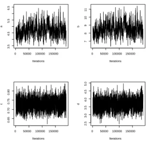
When setting the value of e to 0:1, 0:05, and 0:01, running an hybrid MCMC algorithm leads to a highly stable estimation of the other parameters. The results of this simulation for e = 0:01 are presented in Figures 3 and 4 while the Bayesian estimates of a; b; c; d are given in Table 3 for the di¤erent chosen values of e. The estimates are quite close and the mixing behavior of the MCMC chains seems to be fairly impervious to changes in e. We are therefore satis…ed with this proxy to the full parameter estimation scheme and in the next we will retain a value of 0:01 for e:
Now, for a given sample (x; y), we want to estimate the quantity I = Z 1 0 Z u 0 u z(u; v) ua 1(1 u)b 1vc 1(1 v)d 1(u v)e g(a; b; c; d; e) dv du Z 1 0 Z u 0 1 z(u; v) ua 1(1 u)b 1vc 1(1 v)d 1(u v)e g(a; b; c; d; e) dv du = I3 I4 :
Since this ratio depends on the unknown parameters (a; b; c; d), e being …xed, the natural esti-mator is the Bayes posterior expectation conditional on the sample (x; y), E[Ij(x; y)]. There is
however a di¢ culty in that both integrals I3 and I4 are not available in closed form. We thus
resort to separate evaluations of both integrals, with I3 and I4 estimated by importance
sam-pling in order to ensure …nite variance estimates (Robert and Casella, 2004). The importance
distribution we use is a Dirichlet D( ; e ; ) with > 0, e > 0 and > 0, and density
vi 1(ui vi)e 1(1 ui) 1 ( + e + ) ( ( ) (e ) ( ));
due to the similarity with the target distribution and the warranty of a …nite variance. The importance sampling estimates of both integrals are therefore
e I3= 1 N N X i=1 uai i (1 ui)bi 1vici 1(1 vi)di 1(ui vi)e g(ai; bi; ci; di; e) z(ui; vi)v 1i (ui vi)e 1(1 ui) 1 ( + e + ) ( ( ) (e ) ( )) ; and e I4= 1 N N X i=1 uai 1 i (1 ui)bi 1v ci 1 i (1 vi)di 1(ui vi)e g(ai; bi; ci; di; e) z(ui; vi)v 1i (ui vi)e 1(1 ui) 1 ( + e + ) ( ( ) (e ) ( )) ;
where ((u1; v1); : : : ; (uN; vN)) is an i.i.d. sample from D( ; e ; ) and the (ai; bi; ci; di)’s
constitute the MCMC sample from the posterior distribution of (a; b; c; d) given (x; y).9
The Bayes estimate of I is therefore approximated by the ratio of both importance sampling
Bayes estimates, i.e. eI3= eI4:
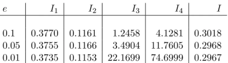
The corresponding estimations of I1; I2; I3; I4 and I are given in Table 4, based on 200; 000
MCMC iterations. For e = 0:1 and e = 0:05, we used the last 190; 000 MCMC iterations in the
summation and = 0:01. For e = 0:01, we used only the last 150; 000 MCMC iterations in the
summation and = 0:001. The estimates of I1; I2 and I are very stable with respect to the
variations of e even if I3 and I4 diverge when e goes to zero.
Recall that the objective probability is 0.5. As shown in Table 2, the average subjective
probability which is given by I1 is around 0:37: The average subjective probability weighted by
the risk tolerance, which is given by I2, is much lower than I1 and is around 0.3. As far as the
link between optimism and risk aversion is concerned, these results indicate the presence of a positive correlation between optimism and risk aversion: more risk averse individuals are more optimistic.
4
Conclusion
In this paper, we have adopted a Bayesian estimation approach in order to analyze the link between risk aversion and optimism and to estimate the risk tolerance weighted average of subjective probabilities (which represents the consensus probability of the group) as well as the unweighted average. In the analyzed survey, while the objective probability is 0.5, the
9
It may sound surprising to mix (ui; vi)’s simulated from the importance function with (ai; bi; ci; di)’s
sim-ulated from the posterior distribution, but the average eI3 (resp. eI4) is converging to the double expectations
estimated (equally-weighted) average subjective probability reveals to be around 0.4 and the estimated average subjective probability weighted by the risk tolerance reveals to be around 0.3. It appears then, on our sample, that the group is pessimistic and more pessimistic than the average individual.
We do not pretend that 0.3 represents the collective subjective probability in a general
setting, nor that 0:4 0:50:5 = 0:2 represents the average level of optimism in all risk-taking
situations in a [ 1; 1] scale. We only claim that the di¤erence between the unweighted and the risk tolerance weighted averages of subjective probabilities is substantial enough to conclude to a behavioral correlation between optimism and risk aversion. Analogously, the di¤erence between the objective probability and the unweighted average of subjective probabilities is substantial enough to conclude to a behavioral bias toward pessimism at the individual level. As a consequence there should be a bias toward pessimism at the collective level. The impact on the equilibrium characteristics should then be towards an increase of the risk premium and a decrease of the risk free rate, which is interesting with regard to the risk premium and risk free rate puzzles.
To identify the origin of the elicited pessimism and correlation between optimism and risk aversion is a delicate question. The observed pessimism might result from an individual learning process, where individuals overestimate bad experiences (see Taylor, 1991) and the intensity of this e¤ect might be related to the individual level of risk aversion. Besides, people seem to be disappointment averse in their choices (Bell, 1985). Disappointment avoidance may re‡ect a self deception mechanism designed to protect self esteem about decision making ability, i.e. a calculated avoidance of unpleasant future feelings (Joseph et al., 1996, Gollier and Muerman, 2006). The elicited pessimism could be interpreted as defensive pessimism, an anticipatory strategy that involves setting defensively low expectations prior to entering a situation so as to defend against loss of self esteem in the event of failure and here again the intensity of this e¤ect might be related to the individual level of risk tolerance. This would require a deeper analysis of the process of belief formation.
References
[1] Abel, A., 1989. Asset prices under heterogeneous beliefs: Implications for the equity pre-mium. Mimeo, University of Pennsylvania.
[2] Barsky R., Juster F.T., Kimball M.S. and Shapiro M.D., 1997. Preference parameters and behavioural heterogeneity. An experimental approach in the health and retirement study. The Quarterly Journal of Economics,112, 537-80.
[3] Bell, D. E., 1985. Disappointment in decision making under uncertainty. Operations Re-search, 33(1), 1-27
[4] Ben Mansour, S., Jouini, E. and C. Napp, 2006. Is there a “pessimistic” bias in individual beliefs? Evidence from a simple survey. Theory and Decision, 2006, 61(4), 345-362. [5] Binswanger, H.P, 1980. Attitudes toward risk: Experimental measurement in rural India.
American Journal of Agricultural Economics, 62 (3), 395-407.
[6] Binswanger, H.P, 1981. Attitudes toward risk: Theoretical implications of an experiment in rural India. Economic Journal , 91, 867-890.
[7] Calvet, L., Grandmont, J.-M., and I. Lemaire, 2002. Aggregation of heterogeneous beliefs and asset pricing in complete …nancial markets. Working Paper.
[8] Cohn R.A., Lewellen W.G, Lease R.C and Schlarbaum G.G, 1975. Individual …nancial risk aversion and investment portfolio composition. Journal of Finance, 30, 605-620.
[9] Detemple, J. and S. Murthy, 1994. Intertemporal asset pricing with heterogeneous beliefs. Journal of Economic Theory, 62, 294-320.
[10] Donkers, B., Melenberg, B. and Van Soest, A., 2001. Estimating risk attitudes using lot-teries: a large sample approach. Journal of Risk and Uncertainty, 22 (2), 165-195.
[11] Dreman, D. N. and M. Berry, 1995. Analyst forecasting errors and their implications for security analysts. Financial Analysts Journal 51, 30-40.
[12] Eisenhauer, J.G. and M. Halek, 2001. Demography of risk aversion. The Journal of Risk and Insurance, 68, 1, 1-24.
[13] Eisenhauer, J.G. and L. Ventura, 2003. Survey measures of risk aversion and prudence. Applied Economics, 35, 1477-1484.
[14] Felton, J., Gibson, B. and D.M. Sanbonmatsu, 2003. Preference for Risk in Investing as a Function of Trait Optimism and Gender. Journal of Behavioral Finance, 33-40.
[15] Francis, J. and D. Philbrick, 1993. Analysts’decisions as products of a multi-task environ-ment. Journal of Accounting Research 31, 216-230.
[16] Fried, D. and D. Givoly, 1982. Financial Analysts’Forecasts of Earnings: A Better Surro-gate for Earnings Expectations. Journal of Accounting and Economics 4, 85-107
[17] Giordani, P. and P. Söderlind, 2005. Is there evidence of pessimism and doubt in subjective distributions? Implications for the risk premium puzzle. Journal of Economic Dynamics and Control, 30(6), 1027-1043.
[18] Gollier, C., 2007. Who Should we Believe? Collective risk-taking decisions with heteroge-neous beliefs. Journal of Risk and Uncertainty. To appear.
[19] Gollier, C. and A. Muerman, 2006. Optimal choice and beliefs with ex Ante savoring and Ex Post disappointment. IDEI working Paper, 201.
[20] Guiso, L. and Paiella, M., 2001. Risk aversion, wealth and background risk. Discussion paper 2728, Center of Economic Policy Research, March.
[21] Hariharan G., Chapman K.S and Domian D.L., 2000. Risk tolerance and asset allocation for investors nearing retirement. Financial Services Review, 9, 159-170
[22] Hartog J., Carbonell A.F., and Jonker N., 2002. Linking measured risk aversion to individ-ual characteristics. Kyklos, 55, 3-26
[23] Jianakoplos, N. A. and Bernasek, A., 1998. Are women more risk averse? Economic Inquiry, 36, 620-30.
[24] Joseph, R., Larrick, R.P, Steele, C.M and Nisbett, R.E., 1996. Protecting the self from the negative consequences of risky decisions. Journal of Personality and Social Psychology, 62, 26-37
[25] Jouini, E. and Napp, C., 2006. Heterogenous beliefs and asset pricing in discrete time: an analysis of pessimism and doubt. Journal of Economic Dynamics and Control, 30, 1233-1260.
[26] Jouini, E. and Napp, C., 2007. Consensus consumer and intertemporal asset pricing with heterogeneous beliefs. Review of Economic Studies. Forthcoming.
[27] Kang, S., J. O’Brien and K. Sivaramakrishnan, 1994. Analysts’interim earnings forecasts: Evidence on the forecasting process. Journal of Accounting Research 32, 103-112.
[28] Li, T., 2006. Heterogeneous beliefs, asset prices, and volatility in a pure exchange economy, Journal of Economic Dynamics and Control, In Press.
[29] Mc Inish, T.H., 1982. Individual investors and risk-taking. Journal of Economic Psychology, 2, 125-136.
[30] McKelvey, R. and T. Palfrey, 1992. An experimental study of the centipede game. Econo-metrica, 60, 803-836.
[31] Mehra, R., and E. Prescott, 1985. The equity premium: A puzzle. Journal of Monetary Economics, 15, 145-162.
[32] Morin, R. A. and Suarez, A. F., 1983. Risk aversion revisited. The Journal of Finance, 38(4), 1201-1216.
[33] O’Brien, P. C., 1988. Analysts Forecasts as Earnings Expectations. Journal of Accounting and Economics 10, 53-88.
[34] Palsson A.M, 1996. Does the degree of risk aversion vary with household characteristics? Journal of Economic Psychology, 17, 771-787.
[35] Powell, M. and Ansic, D., 1997. Gender di¤erences in risk behaviour in …nancial decision making: An experimental analysis. Journal of Economic Psychology, 18, 605-628.
[36] Riley W.B and Chow K.V, 1992. Asset allocation and individual risk aversion. Financial Analysts Journal, 48, 32-37.
[37] Robert, C. P., 2001. The Bayesian Choice, Springer-Verlag, New York.
[38] Robert, C.P. and Casella, G., 2004. Monte Carlo Statistical Methods, Springer-Verlag, New York.
[39] Rubinstein, M., 1976. The Strong Case for the Generalized Logarithmic Utility Model as the Premier Model of Financial Markets. Journal of Finance, 31, 551-571.
[40] Schooley D.K and Worden D.D, 1996. Risk aversion measures: comparing attitudes and asset allocation. Financial Services Review,5, 87-99.
[41] Taylor, S., 1991. Asymmetric e¤ects of positive and negative events: the Mobilization-Minimization Hypothesis. Psychological Bulletin, 110, 67-85.
[42] Wang, H. and Hanna, S., 1997. Does risk tolerance decrease with age? Financial Counseling and Planning, 8, 27-31.
[43] Weil, P., 1989. The equity premium puzzle and the risk free rate puzzle. Journal of Monetary Economics, 24, 401-421.
[44] Wenglert, L. and Rosen, A.S., 2000. Measuring optimism-pessimism from beliefs about future events. Personality and Individual Di¤erences, 28, 717-728.
[45] Zapatero, F., 1998. E¤ects on Financial Innovations on Market volatility when Beliefs are Heterogeneous. Journal of Economic Dynamics and Control, 22, 597-626.
Appendix
Let us …rst de…ne
fG(yjx) =
1
4 fG( 1x; 1)(y) + fG( 2x; 2)(y) + fG( 3x; 3)(y) + fG( 4x; 4)(y) :
The hybrid MCMC algorithm we used in our simulation is described by the following steps: Hybrid MCMC algorithm
Initialization: Simulate a(0); b(0); c(0); d(0) from 4i=1Ga(1; 1)
For i 2 f1; : : : ; ng, simulate (0)i ; p (0) i from Be xi+ a(0); 10 xi+ b(0) Be]0; (0) i [ yi+ c(0); 100 yi+ d(0)
(truncated Beta distribution)
For t = 1; : : ::
1) For i 2 f1; : : : ; ng, simulate (~i; ~pi) from
Be xi+ a(t 1); 10 xi+ b(t 1) Be]0; (t) i [ yi+ c(t 1); 100 yi+ d(t 1) and take (t) i ; p (t) i = ( (~i; ~pi) with probability ( ;p)i (t 1) i ; p (t 1) i with probability 1 ( ;p) i where ( ;p) i = min 0 @ (~i p~i) e(t 1) FBe(c(t 1)+y i;d(t 1)+100 yi;0;1)(~i) ( (t 1)i p(t 1)i )e(t 1)FBe(c(t 1)+y i;d(t 1)+100 yi;0;1)( (t 1) i ) ; 1 1 A
2) Simulate ~a from fG ja(t 1) and take
a(t)= 8 > > < > > : ~
a with probability a= min
0 @ fa(~aj : : :) =fG ~aja (t 1) fa a(t 1)j : : : =fG a(t 1)j~a ; 1 1 A a(t 1) with probability 1 a
3) Simulate ~b from fG jb(t 1) and take
b(t)= 8 > > < > > :
~b with probability b= min
0 @ fb ~bj : : : =fG ~bjb (t 1) fb b(t 1)j : : : =fG b(t 1)j~b ; 1 1 A b(t 1) with probability 1 b
4) Simulate ~c from fG jc(t 1) and take
c(t)= 8 > > < > > : ~
c with probability c= min
0 @ fc(~cj : : :) =fG ~cjc (t 1) fc c(t 1)j : : : =fG c(t 1)j~c ; 1 1 A c(t 1) with probability 1 c
5) Simulate ~d from fG jd(t 1) and take d(t)= 8 > > < > > : ~
d with probability d= min
0 @ fd dj : : : =f~ G djd~ (t 1) fd d(t 1)j : : : =fG d(t 1)j ~d ; 1 1 A d(t 1) with probability 1 d
6) Simulate ~e from fG je(t 1) and take
e(t)= 8 > > < > > : ~
e with probability e= min 0 @ fe(~ej : : :) =fG ~eje (t 1) fe e(t 1)j : : : =fG e(t 1)j~e ; 1 1 A e(t 1) with probability 1 e
After some experimenting, we found that the scales 1 = 1, 2= 10, 3 = 100 and 4 = 1000
F requ enc y -1.0 -0.5 0.0 0.5 1.0 0 50 100 150 200 250 300 350
Figure 1: Distribution of pessimism. This …gure represents the distribution of “pessimism” across our sample. A value of -1 (resp. 1) corresponds to people who think that they will never (resp. always) win at the head or tail game. The value of -0.1, which is endowed with the largest frequency of individuals, corresponds to people who think that they will win (or head will occur) 4 times out of ten.
c E[ OAi wij i 2 c] 1 515.8272 2 703.077 3 608.1076 4 951.7348 5 758.1568 6 1218.167 7 1206.866
Table 1: This table reports for each class c of relative risk aversion the average level over the individuals in that class of the product of absolute risk aversion (under the objective probability,
OAi) by the mean of the income band wi. Kendall’s Tau is equal to 0.71, Spearman’s Rho is
equal to 0.89 and Pearson’s correlation coe¢ cient is equal to 0.89. There is then a positive relationship between the elicited levels of absolute and relative risk aversion.
0 20 40 60 80 100 0 2 4 6 8 10 y x
Figure 2: JITTER representation of the dataset. This …gure reports on the horizontal axis the maximum price individuals are willing to pay in the game with ten draws and on the vertical axis the number of times they think that they will win.
xi E[ CAij xi] 1 0.7732720 2 0.8224625 3 0.7881803 4 0.8831758 5 1.1054212 6 0.9278274 7 1.4897416 8 1.0668114 9 5.1140936
Table 2: Average level of corrected risk aversion for a given level of x (number of times the individual thinks he is going to win). Kendall’s Tau is equal to 0.78 and Spearman’s Rho is equal to 0.9 which indicates a positive link between optimism and corrected risk aversion.
e ^a ^b c^ d^
0.1 4.6305 8.5007 0.7207 3.1777
0.05 4.5005 8.2155 0.7142 3.2730
0.01 4.7623 8.5973 0.7283 3.6653
Table 3: MCMC estimates of a; b; c; d (empirical means over the last 190; 000 points in the MCMC sample out of 200; 000 iterations).
e I1 I2 I3 I4 I
0.1 0.3770 0.1161 1.2458 4.1281 0.3018
0.05 0.3755 0.1166 3.4904 11.7605 0.2968
0.01 0.3735 0.1153 22.1699 74.6999 0.2967
Table 4: MCMC estimates of I1 ,I2, I3; I4 and I based on 200; 000 iterations. It is immediate
0 50000 100000 150000 3 .5 4 .5 5 .5 6 .5 Iterations a 0 50000 100000 150000 7 8 9 10 11 Iterations b 0 50000 100000 150000 0. 65 0. 70 0. 75 0. 80 Iterations c 0 50000 100000 150000 2 .5 3 .0 3 .5 4 .0 4 .5 5 .0 Iterations d
Figure 3: e = 0:01 : evolution of the hybrid MCMC sample over 150; 000 iterations
a D en s ity 3.5 4.0 4.5 5.0 5.5 6.0 6.5 0 .0 0 .2 0 .4 0 .6 0 .8 b D en s ity 6 7 8 9 10 11 0 .0 0 .1 0 .2 0 .3 0 .4 0 .5 c D en s ity 0.65 0.70 0.75 0.80 0.85 0 2 4 6 8 10 14 d D en s ity 2.5 3.0 3.5 4.0 4.5 5.0 0 .0 0 .4 0 .8 1 .2