Approximation algorithms for some vehicle routing problems

Approximation algorithms for some vehicle routing problems

Abstract

We study vehicle routing problems with constraints on the distance traveled by each vehicle or on the number of vehicles. The objective is either to minimize the total distance traveled by vehicles or to minimize the number of vehicles used. We design constant differential approximation algorithms for kVRP. Note that, using the differential bound for Metric 3VRP, we obtain the randomized standard ratio 197

99 + ε, ∀ε > 0. This is an improvement of the best-known bound of 2 given by Haimovich et

al. [12]. For natural generalizations of this problem, called Edge Cost VRP, Vertex Cost VRP, Min Vehicle and kTSP we obtain constant differential approximation algorithms and we show that these problems have no differential approximation scheme, unless P=NP.

Keywords: differential ratio, approximation algorithm, VRP, TSP

1

Introduction

Vehicle routing problems that involve the periodic collection and delivery of goods and services such as mail delivery or trash collection are of great practical importance. Simple variants of these real problems can be modeled naturally with graphs. Unfortunately even simple variants of vehicle routing problems are NP-hard. In this paper we consider approxi-mation algorithms, and measure their efficiencies in two ways. One is the standard measure giving the ratio apx_opt, where opt and apx are the values of an optimal and approximate solu-tion, respectively. The other measure is the differential measure, that compares the worst ratio of, on the one hand, the difference between the cost of the solution generated by the algorithm and the worst cost, and on the other hand, the difference between the optimal cost and the worst cost. Formally, the differential measure gives the ratio α = wor−apx_wor−opt, where wor is the value of the optimal solution for the complementary problem. In [15], the measure 1 − α is considered and it is called there z-approximation. Justification for this measure can be found for example in [1, 6, 27, 15, 20].

The main subject of this paper is differential approximation of routing problems. In these problems n customers have to be served by vehicles of limited capacity from a common

depot. A solution consists of a set of routes, where each starts at the depot and returns

there after visiting a subset of customers, such that each customer is visited exactly once. We refer to a problem as a vehicle routing problem (VRP) if there is a constraint on the (possibly weighted) number of customers visited by a vehicle. This constraint reflects the assumption that the vehicle has a finite capacity and that it collects from the customers

† _{LAMSADE, Universit´e Paris-Dauphine, Place du Marechal de Lattre de Tassigny, 75775 Paris Cedex}

16, France. Email: {bazgan,monnot}@lamsade.dauphine.fr

‡_{Department of Statistics and Operations Research, Tel-Aviv University, Tel Aviv 69978, Israel. E-mail:}

(or distributes among them) a commodity. The goal is to find a solution such that the total length of the routes is as small as possible. In other cases, the vehicle is just supposed to visit the customers, for example, in order to serve them. In such cases we refer to the problem as a TSP problem. We will assume in such cases that the limitation is on the total distance traveled by a vehicle and not on the number of customers it visits, and in this case we search solution with a minimum number of vehicles used.

The problems that are considered here generalize the (undirected) Traveling Sales-man Problem (TSP). Differential approximation algorithms for the TSP are given by Hassin and Khuller [15] and Monnot [20]. We will sometimes use these algorithms to generate approximations for the problems of this paper. However, we note an important difference. In the TSP, adding a constant k to all of the edge lengths does not affect the set of optimal solutions or the value of the differential ratio. The reason is that every solution contains exactly n edges and therefore every solution value increases by exactly the same value, namely nk. In particular, this means that for the purpose of designing algorithms with bounded differential ratio, it doesn’t matter whether d is a metric or not (it can be made a metric by adding a suitable constant to the edge lengths). In contrast, in some of the problems dealt with here, the number of edges used by a solution is not the same for every solution and therefore it may turn out, as we will see, that in some cases the metric version is easier to approximate.

It is easy to see that 2VRP is polynomial time solvable. For k ≥ 3, Metric kVRP was proved NP-hard by Haimovich and Rinnooy Kan [11]. In [12], Haimovich, Rinnooy Kan and Stougie gave a 5

2−2k3 standard approximation for Metric kVRP. We study for the

first time the differential approximability of kVRP. More exactly we give a 1₂ differential approximation for the non-metric case for any k ≥ 3. We improve this bound to 3₅ for

Metric 4VRP and 2

3 for Metric kVRP with 5 ≤ k ≤ 8. We also improve the cases k = 3

and k ≥ 9 to 50

99 − ε, ∀ε > 0 and

25(k−1)

33k − ε, ∀ε > 0 respectively by using a randomized

algorithm. An approximation lower bound of 2219₂₂₂₀ is given here for Metric nVRP with length 1 and 2 using a lower bound of TSP(1,2) [8].

We study a generalization of VRP, called Edge Cost VRP, where the maximum length traversed by each vehicle is bounded. We establish a 1₃ differential approximation for this problem.

Min-Max kTSP is a generalization of TSP where we search to cover the customers by at most k vehicles such that the maximum length traversed by the vehicles is minimum. The metric case of the problem was studied by Fredrickson, Hecht and Kim [9] where they give a 5₂ − 1_k standard approximation algorithm by constructing a reduction from this problem to Metric TSP and using Christofides’ algorithm [4]. We establish a 1₂ differential approximation for Metric Min-Max kTSP and prove that it has no differential approximation scheme, unless P=NP. We also give a standard lower bound of p+1_p for Min-Max bn_pcTSP, for p ≥ 6.

Min-Sum EkTSP is another generalization of TSP where we search to cover the cus-tomers by exactly k vehicles such that the total length is minimum. We show that Metric Min-Sum EkTSP is 2₃ differential approximable and it has no differential approximation scheme unless P=NP.

In Min Vehicle the goal is to minimize the number of vehicles subject to a constraint on the maximum length traversed by any single vehicle. In [19], Li, Simchi-Levi and Desrochers proved that Min Vehicle is not standard 2 approximable, unless P=NP and it is 1 + α

α−2

distance that each vehicle could cover. We first present a 2

3 differential approximation

algorithm and show how to improve the bound to 289₃₆₀for the metric version of Min Vehicle. We also show that even when λ is constant and the lengths are 1 and 2, Min Vehicle has no standard and differential approximation scheme, unless P=NP.

The paper is organized as follows: In section 2 we give the necessary definitions. In section 3 we give a constant differential approximation algorithm for General kVRP, and a better constant differential approximation for the metric case. In section 4 the main result is a constant differential approximation for Edge Cost VRP. In the last three sections we show that Min-Max kTSP, Min-Sum EkTSP and Metric Min Vehicle are constant differential approximable and have no differential approximation scheme, if P 6= NP.

2

Terminology

Given an instance x of an optimization problem and a feasible solution y of x, we denote by val(x, y) the value of the solution y, by opt(x) the value of an optimal solution of x, and by wor(x) the value of a worst solution of x. The differential approximation ratio of y is defined as δ(x, y) = |val(x,y)−wor(x)|_{|opt(x)−wor(x)|} . This ratio measures how the value of an approximate solution val(x, y) is located in the interval between opt(x) and wor(x). In particular, it is equivalent for a minimization problem to prove δ(x, y) ≥ ε and val(x, y) ≤ εopt(x) + (1 −

ε)wor(x).

For a function f , f (n) < 1, an algorithm is a f (n) differential approximation algorithm for a problem Q if, for any instance x of Q, it returns a solution y such that δ(x, y) ≥ f (|x|). We say that an optimization problem is constant differential approximable if, for some constant δ < 1, there exists a polynomial time δ differential approximation algorithm for it. An optimization problem has a differential polynomial time approximation scheme if it has a polynomial time (1 − ε) differential approximation, for every constant ε > 0. We say that two optimization problems are standard (differential) equivalent if a δ differential approximation algorithm for one of them implies a δ standard (differential) approximation algorithm for the other one.

We consider in this paper several routing problems. The problems are defined on a complete undirected graph denoted G = (V, E). The vertex set V consists of a depot vertex 0, and customer vertices {1, . . . n}, and each edge (i, j) ∈ E is endowed with a weight

di,j ≥ 0. We call a such graph a complete valued graph. We refer to the version of the

problem in which d is assumed to satisfy the triangle inequality as the metric case. The output to the problems consists of a p-tour, that is, a set of simple cycles, C1, . . . , Cp, such

that V (C_i) ∩ V (C_j) = {0}, ∀i 6= j, and ∪p_i=1V (C_i) = V . The sequence (0, i, 0) with i 6= 0 is accepted as a cycle. We now describe the problems. For each one we specify the input, the problem’s constraints, and the output.

kVRP

Input: A complete valued graph. Constraint: |Cj| ≤ k + 1, j = 1, . . . , p.

Edge Cost VRP

Input: A complete valued graph and a metric {`e : e ∈ E}, and λ > 0.

Constraint: P_e∈E(Cj)`e ≤ λ, j = 1, . . . , p.

Output: A p-tour minimizing the total weight of the cycles. Vertex Cost VRP

Input: A complete valued graph and a function {c_i ≥ 0 : i ∈ V }, where c_i denotes the cost of the vertex i and λ > 0.

Constraint: P_{i∈V (Cj)}ci ≤ λ, j = 1, . . . , p.

Output: A p-tour minimizing the total weight of the cycles. Min-Max kTSP

Input: A complete valued graph. Constraint: p ≤ k.

Output: A p-tour minimizing the maximum weight of the cycles. Min-Sum EkTSP

Input: A complete valued graph. Constraint: p = k.

Output: A p-tour minimizing the total weight of the cycles. Min Vehicle

Input: A complete valued graph and λ > 0. Constraint: P_e∈E(Cj)de≤ λ, j = 1, . . . , p.

Output: A p-tour minimizing p. Min Distance

Input: A complete valued graph and λ > 0. Constraint: P_e∈E(Cj)de≤ λ, j = 1, . . . , p.

Output: A p-tour minimizing the total weight of the cycles.

For an optimization problem Q with edge lengths, we denote by Q(a, b) the version of Q where weights are between a and b and more specifically Q[t], for t > 1, the variant where b ≤ ta for any a > 0. We will use the following problem:

Min TSP Path(1,2) is the variant of Min TSP(1,2) problem where instead of a tour we ask for a Hamiltonian path of minimum weight. Min TSP Path(1,2) has no differential approximation scheme [22] even if opt = n − 1 and wor = 2(n − 1) where n is the number of vertices since it is proved in [2] that Min TSP(1,2), when the subgraph restricted to edges of length 1 is Hamiltonian and cubic, has no standard approximation scheme.

We will also use the following problems:

partitioning into paths of length k (kPP): Given a graph G = (V, E) with |V | = (k + 1)q, is there a partition of V into q paths P1, . . . , Pq, each path with k + 1 vertices?

2PP has been proved NP-complete in [10] whereas, more generally, the NP-completeness of

kPP is proved in [18] as a special case of the G-partition problem. Thus (n − 1)PP is

the decision version of Hamiltonian Path.

Max weighted partitioning into paths with at most k vertices (Max weighted atmostkPP): Given a weighted complete graph G where each edge (i, j) ∈ E is endowed

with a weight d_i,j ≥ 0, we want to find a partition of vertices into paths P₁, . . . , P_q, each path with at most k vertices (or indifferently k −1 edges) such thatPq_i=1d(Pi) is maximum.

There is an easy reduction proving the NP-hardness of this problem between kPP and Max weighted atmost(k + 1)PP that consist to complete the graph G instance of kPP by edges of weight 0.

A binary 2-matching (also called 2-factor or cycle cover) is a subgraph in which each vertex in V has a degree 2. Since the graph is simple, each cycle has at least three vertices. A minimum binary 2-matching is one with minimum total edge weight. Hartvigsen [14] has shown how to compute a minimum binary 2-matching in O(n3_{) time (see [25] for another}

O(n2_{|E|) algorithm). More generally, a binary f-matching, where f is a vector of size n + 1,}

is a subgraph in which each vertex i of V has a degree fi. A minimum binary f-matching

is one with minimum total edge weight and is computable in polynomial time [5].

3

kVRP

nVRP is standard equivalent to TSP. So, using the result of Sahni and Gonzalez [26] we

deduce that nVRP is not 2p(n)_{standard approximable for any polynomial p, unless P=NP.}

In fact for any k ≥ 5 the problem is as hard to approximate as nVRP.

Theorem 3.1 For all k ≥ 5 (even if k is a function of n), kVRP, is not 2p(n) _standard

approximable for any polynomial p, unless P=NP.

Proof: We use a reduction from partitioning into paths of length k (kPP). Given the graph G = (V, E) on n0 _{= (k + 1)q vertices we construct a graph G}0 _{on n vertices,}

instance of (k + 3)VRP. We add a vertex 0 (the depot) to G and a set A of 2q vertices. We define the function d as follows: di,j = 1, if i ∈ V ∪ {0} and j ∈ A or if (i, j) ∈ E and

i, j ∈ V . Finally, the remaining edges have weight n2p(n)_.

If G contains a decomposition into disjoint paths of k+1 vertices then opt(G0_{) = q(k+4),}

otherwise opt(G0_{) > n2}p(n)_{. So, a 2}p(n)_{standard approximation for (k+3)VRP could decide}

kPP in polynomial time. The conclusion follows.

3.1 General kVRP

When d is a metric, the reduction of TSP to nVRP is straightforward, and it easily follows that computing opt is NP-hard. On the other hand, this reduction between the correspond-ing maximization problems Max TSP and Max nVRP leadcorrespond-ing to the conclusion that computing wor is also NP-hard, does not work. We can easily prove this result by applying a reduction from kPP with weight 1 and 3. The idea of this reduction is to construct from a graph G = (V, E) with |V | = (k + 1)q an instance of kVRP by adding the depot vertex 0 and setting d_e = 3 if e ∈ E and d_e = 1 otherwise. It is easy to verify that the answer to

kPP is positive if and only if wor ≥ q(3k + 2).

In the following we give a 1₂ differential approximation for non-metric kVRP.

We first compute a lower bound LB. Then we generate a feasible solution for G with value good = LB + δ1. Next, we generate another feasible solution of value bad = LB + δ2

approximation where α = wor − good wor − opt ≥ bad − good bad − opt ≥ δ2− δ1 bad − LB = δ2− δ1 δ₂ = 1 − δ1 δ₂, (1)

since for a minimization problem wor ≥ bad ≥ good ≥ opt ≥ LB. To generate LB we replace 0 by a complete graph with a set V0 of 2n vertices and zero length edges. The

distance between a vertex of V0 and a vertex i of V \ V0 is the same as the distance between

0 and i. Denote the resulting graph by G0_{. Compute in G}0 _{a minimum weight binary}

2-matching M0_.

Lemma 3.2 Let LB denote the weight of M0_{, and denote by opt the value of an optimal}

VRP solution. Then opt ≥ LB.

Proof: It is sufficient to show that for any VRP solution in G there exists a binary 2-matching in G0 _{with the same value. Consider an optimal VRP solution in G and let C be}

a cycle in it. Generate in G0 _{a cycle C}0 _{which is as C except that 0 is replaced by two new}

adjacent vertices from V0. Repeat this process for every cycle in the VRP solution, taking

care that the subsets of vertices selected from V0 are disjoint (an optimal solution may only

contain cycles (0, i, 0) for i = 1, . . . , n and in such a case, we need to use all vertices of V0).

In the last cycle insert all the remaining vertices of V0. The result is a binary 2-matching

since every cycle has at least three vertices and the cycles are disjoint and cover V . Since the value of cycle C0 _{is the same as the value of C, the optimum of VRP is greater than or}

equal to the minimum binary 2-matching.

Lemma 3.3 A binary 2-matching M0 _{of G}0 _{can be transformed in polynomial time into a}

set M of cycles covering vertices of G with the same weight.

Proof: If a cycle of M0 _{does not contain a vertex of V}

0 then this cycle is considered in

M . If a cycle of M0 contains more than one consecutive vertices from V0 then replace these

vertices by one vertex of V0. Consider in the following a cycle C0 of M0 containing at least

one vertex from V0 and one from V (G0)\V0. Suppose that C0 = (v01, µ1, v02, µ2, . . . , vt0, µt, v01)

where paths µ1, . . . , µtcontain only vertices from V (G0) \ V0. Then M will contain t cycles

(0, µ1, 0), (0, µ2, 0), . . . , (0, µt, 0) that have the same weight as C0.

We suggest the following algorithm. W.l.o.g., we suppose that the current cycle is (0, 1, . . . , m, 0).

Algo Differential VRP

1 Compute LB the weight of a minimum weight binary 2-matching M0 _{in G}0_;

2 Transform M0 _{into M = {C}

1, . . . , Cp}, using Lemma 3.3;

3 For every cycle Ci= (1, . . . , mi, 1) of M do

3.1 If mi≡ 0 mod 2 then

3.1.2 sol_i,2 := {(0, m_i, 1, 0), (0, 2, 3, 0), . . . , (0, m_i− 2, m_i− 1, 0)};

3.2 If mi≡ 1 mod 2 then

3.2.1 soli,1 := {(0, 1, 2, 0), (0, 3, 4, 0), . . . , (0, mi− 4, mi− 3, 0)}

∪{(0, m_i− 2, m_i− 1, m_i, 0)};

3.2.2 soli,2 := {(0, mi, 1, 0), (0, 2, 3, 0), . . . , (0, mi− 3, mi− 2, 0)} ∪ {(0, mi− 1, 0)};

4 For every cycle Ci= (0, 1, . . . , mi, 0) of M with mi > k do

4.1 If mi≡ 0 mod 2 then

4.1.1 Construct soli,1= {(0, 2, 3, 0), . . . , (0, mi−2, mi−1, 0)}∪{(0, 1, 0), (0, mi, 0)};

4.1.2 Construct soli,2= {(0, 1, 2, 0), . . . , (0, mi− 1, mi, 0)};

4.2 If mi≡ 1 mod 2 then

4.2.1 Construct soli,1= {(0, 2, 3, 0), . . . , (0, mi− 1, mi, 0)} ∪ {(0, 1, 0)};

4.2.2 Construct soli,2= {(0, 1, 2, 0), . . . , (0, mi− 2, mi− 1, 0)} ∪ {(0, mi, 0)};

5 For every cycle C_i= (0, 1, . . . , m_i, 0) of M with m_i ≤ k do sol_i,1= sol_i,2 = C_i; 6 Output AP X = ∪p_i=1argmin{d(soli,1), d(soli,2)};

Theorem 3.4 Algo Differential VRP is a 1₂ differential approximation algorithm for kVRP, with k ≥ 3.

Proof: Consider an arbitrary cycle Ciof M and let addi,j denote the added weight of soli,j

for j = 1, 2 with respect to the length of Ci. Note that since M was computed to have a

minimum weight, addi,j ≥ 0 and we have d(soli,j) = d(Ci) + addi,j for j = 1, 2.

On the other hand, let badi be the weight of the feasible solution soli,3 defined by Ci

if 0 ∈ Ci and |Ci| ≤ k + 1 and by {(0, 1, 0), . . . , (0, mi, 0)} otherwise; in any case, we have

badi = d(Ci) + addi,1+ addi,2

Figure 1 and 2 give an illustration of these solutions when Ci= (1, . . . , mi, 1) and mi = 6

and respectively mi = 3. Sum these inequality over i and let δ1=Ppi=1min{addi,1, addi,2}

and δ₂ =Pp_i=1(add_i,1+ add_i,2). We have δ₂ ≥ 2δ₁, LB = d(M ) =Pp_i=1d(C_i) and wor ≥

P_p

i=1badi. So, the theorem is proved by (1).

When we use bounded metrics (i.e., when the maximum weight dmax is not very far

from the minimum weight d_min), we are able to give some relations between differential and standard ratios. Bounded metric variants of TSP were studied by Papadimitriou and Yannakakis [24] and more recently by Papadimitriou and Vempala [23], and Engebretsen and Karpinski [8]. In the following, we denote by kVRP[t] the version of kVRP satisfy-ing dmax

dmin ≤ t for some t > 1.

Theorem 3.5 A δ differential approximation algorithm for kVRP[t] is also a δ+(1−δ)2tk k+1

1 2 3 4 5 6 6 1 1 1 6 4 5 ₅ 5 sol3 sol2 sol1 C 4 6 2 2 2 4 3 3 3 Figure 1: m = 6 3 2 2 2 3

C sol1 sol2 sol3

1 1 1 3 1

Figure 2: m = 3

Proof: Let G = (V, E) be a graph where V = {0, . . . , n} and dmax

dmin ≤ t for some t > 1. An

optimal solution for G contains at least n + dn_ke edges since it has at least dn_ke cycles, and

then we have:

opt ≥ ndmin(1 + k)

k . (2)

On the other hand, any solution of G contains at most 2n edges and then, we deduce the following upper bound for the worst solution:

wor ≤ 2dmaxn. (3)

Finally, regrouping inequalities (2) and (3) and since we have dmax≤ tdmin, we obtain the

inequality: wor ≤ 2t k k+1opt.

Let apx be a δ differential approximation for kVRP[t]. Using the previous inequality we deduce:

apx ≤ δopt + (1 − δ)wor ≤ δopt + (1 − δ)2t k

k + 1opt. (4)

Using the previous theorems we deduce some new standard results for kVRP[t]. More exactly, we obtain a 7₂−_k+13 standard approximation for kVRP[3] and a 9₂−_k+14 standard approximation for kVRP[4].

3.2 Metric kVRP

The first part of this section starts with some positive differential approximation results and ends with a negative result. In the second part, we present an improvement of the best known approximation algorithm for 3VRP.

3.2.1 Differential approximation results

When d is a metric, computing a worst solution becomes easy as shown by the next lemma: Lemma 3.6 wor = 2Pn_i=1d0,i

Proof: Let sol be a feasible solution and denote by (0, 1, . . . , mi, 0) one of these cycles.

We replace it by (0, 1, 0), . . . , (0, m_i, 0) and by the triangle inequality, this change does not

increase the value of the solution. So, we can repeat it on each cycle and finally obtain the solution (0, 1, 0), . . . , (0, n, 0).

In Theorem 3.4 we have shown that kVRP is 1₂ differential approximable. We now show that in the metric case, the same bound can be achieved by a simpler algorithm.

We compute a minimum weight perfect matching M on the subgraph induced by

{1, . . . , n}, if n is even, or by {0, 1, . . . , n} if n is odd. We link each endpoint different

of 0 of M to the depot. We claim that

opt ≥ 2d(M ). (5)

Indeed, consider an optimum solution for kVRP. Walk around it and shortcut in order to obtain a Hamiltonian cycle C on {0, 1, . . . , n} if n is odd and a Hamiltonian cycle C on

{1, . . . , n} if n is even. We have opt ≥ d(C) by the triangle inequality and this cycle is the

sum of two perfect matchings which are greater than or equal to M .

Using (5), Lemma 3.6 and the construction of the approximate solution, we obtain:

apx = d(M ) +

n

X

i=1

d0,i ≤ 1₂opt +1₂wor , (6)

proving that the result is a 1₂ differential approximation.

Theorem 3.7 Metric kVRP is δ·k−1_k differential approximable, where δ is the differential approximation ratio for Metric TSP.

Proof: Our algorithm modifies the Optimal Tour Partitioning heuristic of Haimovich, Rinnooy Kan and Stougie [12]: first construct a tour T of value val(T ) on V using the δ differential approximation algorithm for TSP. W.l.o.g., assume that this tour is described by the sequence (0, 1, . . . , n, 0). We produce k solutions sol_i for i = 1, . . . , k and we select the best solution. The first cycle of soli is formed by the sequence (0, 1, . . . , i, 0) and then

each other cycle (except possibly the last) of soli has exactly k consecutive vertices (for

instance, the second cycle is (0, i + 1, . . . , i + k, 0)) and finally, the last cycle is formed by the unvisited vertices (connecting n to the depot 0). Denote by apxi for i = 1, . . . , k the

values of the solution soli and by apx the value of the best one.

In the union of solutions sol₁, . . . , sol_k each edge of T \ {(0, 1), (0, n)} appear exactly (k − 1) times and each edge (0, j) for j 6= 1, n appears exactly twice. Finally, edges (0, 1) and (0, n) appear exactly (k + 1) times. Since worV RP = 2Pni=1d0,i by Lemma 3.6, we

deduce: apx ≤ 1 k k X i=1

Since T is a δ differential approximation then

val(T ) ≤ (1 − δ)worT SP + δoptT SP. (8)

Since it is possible to construct from an optimum solution of VRP a solution of TSP with a smaller value (using the triangle inequality), it follows that

optT SP ≤ optV RP (9)

Also, by connecting the depot twice with each customer, we can construct from a solution of TSP a solution of VRP with a greater value, and therefore

worT SP ≤ worV RP (10)

Using (7)-(10) we obtain that

apx ≤ δk − 1 k optV RP + µ 1 − δk − 1 k ¶ wor_{V RP}.

Since the best known differential approximation algorithm for TSP is 2

3 [15, 20] then

the algorithm of Theorem 3.7 is an 2₃ ·k−1_k differential approximation algorithm for metric

kVRP. For k > 4 this is an improvement over the bound of 1

2 given by Theorem 3.4 for

the general (non-metric) kVRP.

We will proceed now to improve the bound given in Theorem 3.7 by using a generic algorithm. When we deal with a cycle of size m we consider the vertices modulo m.

Algo Differential MetrickVRP

1 Find a partition of V \ {0} by cycles M = {C1, . . . , Cp} using a Preprocessing

algorithm;

2 For every cycle Ci= (1, . . . , mi, 1) of M with mi= kq + r, 0 ≤ r < k do

2.1 For j = 1 to mi do

2.1.1 Let (µ1, . . . , µdmi_k e) = Ci\[{(j, j+1)}∪{(j+r+`k, j+r+1+`k) : 0 ≤ ` < q}];

2.1.2 Construct soli,j = ∪d

mi k e

`=1 {(0, µ`, 0)};

2.2 Let soli = argmin{d(soli,1), . . . , d(soli,mi)}

3 Output AP X = ∪p_i=1soli;

By using the construction of solutions soli,1, . . . , soli,mi, we easily deduce the following

lemma:

Lemma 3.8 Consider a cycle Ci = (1, . . . , mi, 1) of M with mi = kq + r, 0 ≤ r < k. We

(i) Pmi j=1d(soli,j) = (mi− q)d(Ci) + 2q P_mi j=1d(0, j) if r = 0. (ii) Pmi j=1d(soli,j) = (mi− q − 1)d(Ci) + 2(q + 1) P_mi j=1d(0, j) if r 6= 0.

Proof:(i): soli,j contains dm_kie = q cycles for every j = 1, . . . , mi. Thus, in ∪mj=1i soli,j, each

edge of Ci appears exactly mi− q times and each edge (0, j) appears exactly 2q times.

(ii): soli,j contains dm_kie = q + 1 cycles for every j = 1, . . . , mi. So, the same argument

as previously shows that each edge of Ci appears exactly mi− (q + 1) times and each edge

(0, j) appears exactly 2(q + 1) times in ∪mi

j=1soli,j.

Theorem 3.9 Metric 4VRP is 3₅ differential approximable and Metric kVRP is 2₃ differential approximable with 5 ≤ k ≤ 8.

Proof: Our preprocessing algorithm works as follows: we compute a minimum weight binary 2-matching M = (C1, . . . , Cp) on the subgraph induced by V \ {0}. Consider a cycle

Ci= (1, . . . , mi, 1) of M with mi= kq + r and let wori= 2Pmj=1i d0,j.

Assume q = 0. Since the best solution (i.e., sol_i) is better than the average one, we obtain using Lemma 3.8:

d(sol_i) ≤ r − 1 r d(Ci) + 1 rwori = 1 r(wori− d(Ci)) + d(Ci) . (11)

Since wori ≥ d(Ci) by the triangle inequality and r ≥ 3 (Ci contains at least 3 vertices),

we deduce:

d(sol_i) ≤ 2

3d(Ci) + 1

3wori . (12)

Now, assume q ≥ 1. If r = 0, then we deduce:

d(soli) ≤k − 1_k d(Ci) +_k1wori≤ 2₃d(Ci) +1₃wori (13)

since k ≥ 3. Otherwise, we have r ≥ 1 and we obtain:

d(soli) ≤ _{kq + r}q + 1 (wori− d(Ci)) + d(Ci)

and we deduce since r, q ≥ 1:

d(soli) ≤ k − 1_{k + 1}d(Ci) +_{k + 1}2 wori (14)

On the one hand, it is possible to construct from an optimum solution of Metric VRP a feasible solution of TSP on the subgraph induced by V \ {0} (by shortcutting) with a smaller value and we deduce d(M ) =Pp_i=1d(Ci) ≤ optT SP ≤ optV RP. On the other hand

wor = Pq_i=1wori. Finally, by summing over i the inequalities (12), (13) and (14) and by

distinguishing the case k = 4 and k > 4 we obtain the expected result.

The algorithm of Theorem 3.9 works for any k ≥ 3 and it gives the ratio 1

2 for Metric

3VRP and 2₃ for k ≥ 9. We now improve the previous bound for k = 3 and k ≥ 9 using another preprocessing algorithm. But surprisingly, this algorithm computes an approximate TSP with maximum weight.

Observation 3.10 The differential and standard approximation ratios for Max weighted atmostkPP coincide. Indeed, we have wor = 0 since {Pi}i∈V where Pi = {i} is a feasible

solution.

This problem is very close to Metric kVRP when we deal with differential ratio: Theorem 3.11 For any k ≥ 3, Max weighted atmostkPP and Metric kVRP are

differential equivalent.

Proof: In order to reduce Metric kVRP to Max weighted atmostkPP, consider an instance G of Metric kVRP with n customers. We construct an instance I0 _{of Max}

weighted atmostkPP as follows: we delete the depot 0 and consider the graph Kn and

set d0

x,y = d0,x+ d0,y − dx,y for any vertices x, y ∈ V \ {0}. By the triangle inequality,

d0

x,y ≥ 0. d0x,y denotes the saving gained with respect to the worst solution, by joining x

and y in a cycle rather then reaching each of them from the depot. We have a one to one correspondence between a path P = (1, . . . , j) using at most k vertices in I0 _{and the cycle}

C = (0, 1, . . . , j, 0) with at most k customers in G. Moreover, d0_{(P ) = 2}Pj

i=1d0,i− d(C).

Finally, we also have a one to one correspondence between feasible solutions of these two problems, and since wor = 2Pn_i=1d_0,i, for any solution of G of value val we have

val0 = worV RP − val. (15)

Conversely we reduce Max weighted atmostkPP to Metric kVRP. Let G and d be an instance of Max weighted atmostkPP. We add a depot 0 and we set: d0_0,i = maxe∈Ede, ∀i ∈ V and d0i,j = 2 maxe∈Ede− di,j, ∀i, j ∈ V . The rest of the proof is similar.

Let ρ be the standard approximation ratio for Max TSP. The current best value for ρ is 25₃₃ obtained by a randomized algorithm in [17].

Theorem 3.12 Metric kVRP is (25₃₃k−1_k − ε) differential randomized approximable for k ≥ 3 and any ε > 0.

Proof: Let G be an instance of Metric kVRP with n customers and let ε > 0. In order to obtain a good solution for G, we apply algorithm Algo Differential MetrickVRP where the preprocessing is a tour T = C₁. This tour is produced by the algorithm from [17] applied on the instance I0 _{= (K}

n, d0) with n = kq + r obtained from G as in Theorem 3.11,

that is a 25₃₃ randomized approximation. Using the definition of weight d0 _{and the Lemma}

3.8, we obtain:

wor_{V RP} − apx = max

1≤j≤nd 0_(sol 1,j) ≥ P_n j=1d0(sol1,j) n ≥ ( k − 1 k − ε)d 0_(C 1).

when q ≥ k−1_εk2 − 1_k. Otherwise, we exhaustively solve the problem.

On the other hand, an optimal solution of Max weighted atmostkPP on I0 _{can be}

used to construct a feasible solution of Max TSP on I0by joining the endpoints of the paths. Hence optM axT SP ≥ optMax weighted atmostkPP. Finally, by using the 25₃₃ standard

approxi-mation algorithm for Max TSP for obtaining the tour T , we have d0_(C

1) ≥ 25₃₃optM axT SP

In particular, we obtain a (50

99− ε) differential randomized approximation for Metric

3VRP, that is better than the 1₂ differential approximation given in Theorem 3.4. It also improves the result of Theorem 3.9 for k ≥ 9 since we obtain the differential ratio

δ = 25(k−1)_33k − ε > 2

3 for Metric kVRP. For instance, this ratio is 200297 ' 0.67 for k = 9.

We summarize in the following the differential results that we obtain for Metric kVRP:

• Metric 3VRP is (50

99 − ε) differential randomized approximable for any ε > 0.

• Metric 4VRP is 3₅ differential approximable.

• Metric kVRP is 2₃ differential approximable for 5 ≤ k ≤ 8.

• Metric kVRP is (25₃₃k−1_k − ε) differential randomized approximable for any k ≥ 9

and for any ε > 0.

Finally, note the similarity between the results given in Theorem 3.7 and the one given in Theorem 3.12. They both deal with the reduction in approximation from Metric

kVRP to Max TSP (Max TSP and Min Metric TSP are equivalent with respect to

the differential ratio [20]) and the expansion is very similar δk−1_k for Theorem 3.7 and

ρk−1

k − ε for Theorem 3.12. The only difference is on the measure used: The first reduction

considers the differential ratio for the two problems whereas the second one considers the standard ratio for Max TSP. Actually, the standard ratio ρ = 25₃₃ is better than differential ratio δ = 2

3 for Max TSP and more generally the best standard ratio ρbest for Max TSP

will be always better than the best differential ratio δbest(i.e., ρbest ≥ δbest) since we have a

trivial reduction from any maximization problem to itself transforming a differential result into a standard result (see Lemma 1.3 in Monnot [20]), leading to the conclusion that the reduction of Theorem 3.12 is better. Nevertheless, if the optimal result is ρbest= δbest then

the reduction of Theorem 3.7 will be better.

Since nVRP and TSP are standard equivalent, from the result of Papadimitriou and Yannakakis [24] we deduce immediately that nVRP(1,2) has no standard approximation scheme unless P = NP. Also TSP(1,2) has no differential approximation scheme [21] but we cannot deduce immediately that nVRP(1,2) has no differential approximation scheme since wor_{nV RP} and wor_{T SP} may be very far. However, we prove in the following a lower bound for the differential approximation of nVRP(1,2).

Theorem 3.13 nVRP(1, 2) is not (2219

2220 + ε) differential approximable, for any constant

ε > 0, unless P=NP.

Proof: Since wor_{nV RP} ≤ 4n ≤ 4opt_{nV RP}, a δ differential approximation for nVRP(1, 2) gives a δ +4(1−δ) standard approximation for nVRP(1, 2). Using the negative result given in [8] that TSP(1,2) is not 741₇₄₀ − ε standard approximable, we obtain the expected result.

3.2.2 Some standard approximation results

Despite these observations, by using Theorem 3.9 for Metric kVRP and Theorem 3.5 we establish better standard approximation ratio than Haimovich, Rinnooy Kan and Stougie

(i.e., (5

2 −2k3) standard approximation) when we deal with bounded metrics, i.e., dmax ≤

tdmin. More exactly, Metric 4VRP[2] is47₂₅standard approximable and Metric kVRP[2]

is (2 − _3(k+1)4 ) standard approximable for k ≥ 5.

We now describe some results concerning the standard approximability of Metric

kVRP. In [12], a (5₂ − _2k3 ) standard approximation for Metric kVRP is obtained by reduction to Metric TSP and using Christofides’ algorithm.

The following theorem gives a reduction transforming a standard polynomial time ap-proximation scheme into a differential one, even if we deal with unbounded metrics (dmax

dmin

is not upper bounded).

Theorem 3.14 A δ differential approximation algorithm for Metric kVRP is also a

k − δ(k − 1) standard approximation algorithm.

Proof: Consider an optimal solution for an instance G of Metric kVRP and w.l.o.g. denote by (0, 1, . . . , mi, 0) one of its cycles. Using the triangle inequality, the length of this

cycle is at least 2max{d0,i : i = 1, . . . , mi} ≥ 2_kPm_i=1i d0,i. Summing over each cycle, we

obtain using Lemma 3.6:

opt ≥ 2 k n X i=1 d0,i= wor_k . (16)

Let apx be a δ differential approximation for G. Using the inequality (16) we deduce:

apx ≤ δopt + (1 − δ)wor ≤ δopt + k(1 − δ)opt. (17)

Using Theorem 3.14, Observation 3.10 and Theorem 3.12 we obtain: Corollary 3.15 Metric 3VRP is (3 −4

3ρ + ε) standard approximable for all ε > 0 where

δ is the standard approximation ratio for Max TSP.

More exactly, since ρ = 25₃₃ [17] we obtain the bound 197₉₉ ' 1.99 that is an improvement

of the 2 standard approximation of Haimovich et al. [12].

4

Edge Cost VRP

We assume now that a cost ` satisfying the triangle inequality is associated with any edge, and the solution must satisfy that the total cost on each cycle does not exceed λ.

Note that if we do not assume that ` is a metric then even deciding whether the problem has any feasible solution is NP-complete. For a proof see Theorem 7.1 below. Therefore, we assume that ` satisfies the triangle inequality, and to ensure feasibility we also assume that 2`0,i≤ λ for i = 1, . . . , n.

Theorem 4.1 Edge Cost VRP is 1₃ differential approximable.

Proof: We start with a binary 2-matching as described in Lemma 3.2 except that the initial graph is not a complete undirected graph G but a partial graph G0 of it built by deleting the edges (i, j) for i 6= 0 and j 6= 0 such that `0,i + `i,j + `j,0 > λ. Observe

that M is still a lower bound of an optimal solution of Edge Cost VRP. Then, we apply the algorithm Algo Differential VRP except that we change steps 3.2, 4, 5 and 6. The step 3.2 becomes the following: we produce mi solutions soli,1, . . . , soli,mi where

sol_i,j = {(0, j + 1, j + 2, 0), . . . , (0, j − 2, j − 1, 0)} ∪ {(0, j, 0)} for j = 1, . . . , m_i.

The steps 4 and 5 become respectively : ”for every cycle Ci = (0, 1, . . . , mi, 0) of M with

P

e∈E(Ci)`e > λ (resp.

P

e∈E(Ci)`e ≤ λ) do ...”, whereas the step 6 becomes: the solution

AP X is the solution obtained by concatenating the shortest of sol_i,j for each cycle C_i. Observe that in step 3.2, each edge of Ci appears exactly bm₂ic times in (∪j≤misoli,j)

and each edge (0, j) appears exactly mi+ 1 times. Thus, since mi≥ 2, the same arguments

as in Theorem 3.4 proved that AP X is a 1₃ differential approximation.

In [12], the authors consider two versions of kVRP with additional constraint on the length of each cycle. In the first problem that we will call here Vertex Cost VRP, each customer has a cost and we want to find a solution such that the total customer cost on each cycle does not exceed a given bound λ. In the second, called in [19] Min metric Distance, we want to find a solution such that the total cost on each cycle does not exceed a given bound λ. For each of these two problems, we give a reduction preserving differential approximation scheme from Edge Cost VRP.

Lemma 4.2 A δ differential approximation solution for Edge Cost VRP (respectively,

metric case) is also a δ differential approximation for Vertex Cost VRP (respectively, metric case).

Proof: Let G = (V, E) with d, c and λ > 0 be an instance of Vertex Cost VRP. We construct an instance of Edge Cost VRP as follows. The graph and the function d are the same whereas the function ` is defined by: `i,j = ci+c₂ j where we assume that c0 = 0.

This function satisfies the triangle inequality. Moreover, let C be a cycle linking the depot to a subset of customers. We haveP_{i∈V (C)}ci≤ λ iff

P

e∈E(C)`e≤ λ.

Corollary 4.3 Vertex Cost VRP is 1

3 differential approximable.

Min Metric Distance is a particular case of Edge Cost VRP where the function ` is exactly the function d. Thus, from Theorem 4.1 we deduce the corollary:

Corollary 4.4 Min Metric Distance is 1₃ differential approximable.

Edge Cost VRP and Vertex Cost VRP have neither standard nor differential approximation scheme unless P = NP since these two problems contain nVRP.

5

Min-Max kTSP

The metric case of the problem was studied by Fredrickson, Hecht and Kim [9] where they give a 5₂ −_k1 standard approximation algorithm by constructing a reduction from this problem to Metric TSP and using Christofides’ algorithm [4].

Theorem 5.1 Min-Max rTSP is not 2p(n) _{standard approximable for any polynomial p}

Proof: We reduce Hamiltonian Path problem to Min-Max rTSP. We start with the reduction described in Theorem 3.1 with k = n − 1 and q = 1 and the weight n2p(n) _is

replaced by (n + 3)2p(n) _{(recall that the (n − 1)PP problem is the Hamiltonian Path}

problem) and we apply r times this reduction (so, the final graph consists of depot and r copies of G and set A of 2r vertices). Thus, a 2p(n) _{standard approximation for Min-Max}

rTSP could decide Hamiltonian Path, that is proved NP-hard in [10].

We now turn to the metric case. We give a 1₂ differential approximation algorithm for Metric Min-Max kTSP, k ≥ 2 and we show that the problem has neither standard nor differential approximation scheme unless P=NP.

Theorem 5.2 Metric Min-Max 2TSP is 1₂ differential approximable.

Proof: Consider a tour T = (0, . . . , n, 0) of G. Let i be the smallest index such that

P_i

j=0dj,j+1≥ d(T )₂ . We consider the solution C1 = (0, 1, . . . , i, 0) and C2 = (0, i + 1, . . . , n, 0).

Note that d(C₁) − d_0,i= i−1 X j=0 d_j,j+1≤ d(T ) 2 and d(C₂) − d_0,i+1 = d(T ) − i X j=0 d_j,j+1≤ d(T ) −d(T ) 2 = d(T ) 2 .

So, max{d(C1), d(C2)} ≤ d(T )₂ + max{d0,i, d0,i+1} ≤ wor₂T SP + opt2T SP₂ . Since a worst

tour on V with the value worT SP is a feasible solution for 2TSP then wor2T SP ≥ worT SP.

Thus, max{d(C1), d(C2)} ≤ wor2T SP₂ +opt2T SP₂ .

Corollary 5.3 Metric Min-Max kTSP is 1

2 differential approximable.

Proof: The previous algorithm is a 1₂ differential approximation for general k ≥ 3 since we have also workT SP ≥ worT SP and max{d0,i, d0,i+1} ≤ optkT SP₂ .

Theorem 5.4 Min-Max kTSP(1,2), k ≥ 2, has neither standard nor differential

polyno-mial time approximation scheme, unless P=NP.

Proof: Assume that Min-Max kTSP(1,2) has a standard polynomial time approximation scheme called Aε. We prove that Min TSP(1,2) on instances when the subgraph restricted

to the edges of length 1 is Hamiltonian, has a standard polynomial time approximation scheme. This is a contradiction with the result of [2] (page 99).

Let 0 < ε < 1 and let G be a complete graph on n = q · k + r, 0 < r ≤ k vertices, with edges of length 1 and 2, an instance of Min TSP(1,2) such that the subgraph restricted to the edges of length 1 is Hamiltonian. W.l.o.g., we assume q ≥ 12_ε (otherwise, an exhaustive search solves the problem); thus 4 ≤ q·ε₃ . We construct an instance G0 _{of Min-Max kTSP}

adding to G a depot, the vertex 0, and we set the distance between 0 and a vertex i of G to 2. It is easy to see that opt(G) = optT SP(G) = n and opt(G0) = optM in−M ax kT SP(G0) = q + 4

since the optimum of G0 _{is obtained when the Hamiltonian cycle is divided in k paths where}

the difference of sizes is at most 1.

In order to obtain an (1 + ε) approximation for G, we apply algorithm Aε

3 which finds a solution of G0 _{with value val}0 _{≤ (1 +}ε

in G putting together the paths induced by the solution in G and linking these paths by edges of length at most 2. This solution has the value val ≤ k(val0_{− 4) + 2k ≤ k · val}0_{. So,}

val ≤ k(1 +ε 3)(q + 4) = k · q + 4k + ε 3 · 4k + ε 3· k · q ≤ k · q + ε · k · q ≤ (1 + ε)opt. In order to see that Min-Max kTSP has no differential approximation scheme, we show that if it was the case then Min-Max kTSP on the particular instances that we consider above would have a standard approximation scheme. Suppose that Min-Max kTSP has a differential approximation scheme Aδ, ∀δ, 0 < δ < 1. So, Aδ gives a solution for G0 with

a value val ≤ δopt(G0_{) + (1 − δ)wor(G}0_{). For the above instances G}0 _{of Min-Max kTSP,}

opt(G0_{) =} n−r

k +4 and wor(G0) ≤ 2(n−1)+4 ≤ 2kopt(G0). Thus, val ≤ [δ+2k(1−δ)]opt(G0),

and for an (1 + ε) standard approximation solution for an instance of Min-Max kTSP,

∀ε > 0, we apply Aδ with δ = 1 −_2k−1ε .

For certain cases we can give inapproximability gaps, for examples, when we have bn₆c

vehicles we can prove that the problem is not 7

6 approximable and more generally we obtain:

Theorem 5.5 Min-Max bn

kcTSP(1,2), k ≥ 6 is not k+1k − ε standard approximable for

any ε > 0, unless P=NP.

Proof: We use a reduction from (k − 4)PP with k ≥ 6. We use the reduction described in Theorem 3.1 except that we replace the distances n2p(n)by distances 2. Then, if G contains a decomposition in paths of length k − 4 then opt(G0_{) = k, otherwise opt(G}0_{) ≥ k + 1. So,}

a k+1_k − ε standard approximation for Min-Max bn_kcTSP(1,2) could decide (k − 4)PP in

polynomial time.

6

Min-Sum EkTSP

Bellmore and Hong [3] showed that when the constraint p = k is replaced by p ≤ k, then Min-Sum kTSP is standard equivalent to TSP on an extended graph. This is true even for the directed version of the problem and when there is a cost associated with activating a salesman. For our case the transformation simply involves replacing the depot vertex 0 by k vertices of zero distance. Also, the metric case of the p ≤ k version is not of interest since the solution is just a single cycle (thus, we deal with the case p = k and Min-Sum EkTSP denote this problem).

Min-Sum EkTSP is differential equivalent to Metric Min-Sum EkTSP. This obser-vation follows since the number of edges in every solution is the same (like in the TSP case). Hence, we add a constant to all the edge lengths and achieve the triangle inequality without affecting the best and worst solutions.

Similarly, Min-Sum EkTSP is differential equivalent to Max-Sum EkTSP.

Theorem 5.1 can be adapted in order to prove that Min-Sum EkTSP is not 2p(n)

standard approximable, for any polynomial p, unless P=NP. We now give the main results of this section.

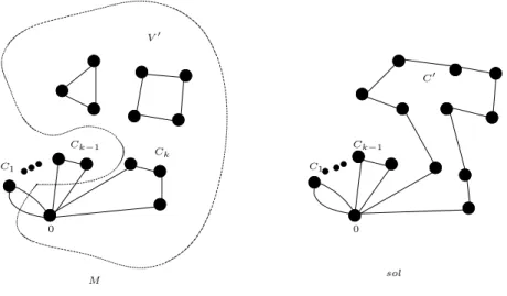
Theorem 6.1 Metric Min-Sum EkTSP is 2₃ differential approximable, ∀k ≥ 1.

Proof: Let G and d be an instance of Metric Min-Sum EkTSP. Add to every edge incident with the depot a parallel copy. Compute a minimum binary f -matching M =

C1 Ck−1 C1 Ck−1 C_k C0 0 0 M sol V0

Figure 3: M and sol

{C1, . . . , Cp} (C1, . . . , Ckdenote the cycles of M containing the depot 0) on G where f (0) =

2k and f (v) = 2 for v ∈ V \ {0}. Compute by using a 2

3 differential approximation

algorithm of [15] or [20] a solution C0 _{for TSP on the subgraph G}0 _{of G induced by V}0 ₌

V \ (∪k−1_i=1V (Ci)) ∪ {0}. The approximate solution sol for Metric Min-Sum EkTSP

is composed of C0 _{and the cycles C}

1, . . . , Ck−1. See Figure 3. Since M is a minimum

binary f -matching M on G then M0 _{= M \ (∪}k−1

i=1Ci) is an optimum binary 2-matching

on G0_{. Let r =} Pk−1

i=1d(Ci). It is proved in [15] or [20] that the TSP algorithm gives a

solution satisfying val ≤ 2

3d(M0) +13worT SP(G0). Since workT SP(G) ≥ worT SP(G0) + r and

optkT SP(G) ≥ d(M0) + r, we deduce that the value of sol satisfies:

apx = val + r ≤ 2 3[d(M 0_{) + r] +} 1 3[worT SP(G 0_{) + r] ≤} 2 3optkT SP(G) + 1 3workT SP(G)

Theorem 6.2 Unless P=NP, Min-Sum EkTSP(1,2) has no standard and differential

ap-proximation scheme for any k ≥ 2.

Proof: We reduce Min TSP Path (1,2) on instances where the subgraph G1 with edges

of length 1 is cubic and Hamiltonian to Min-Sum E2TSP(1,2). From a graph G = (V, E) on n vertices, we construct a graph G0 _{instance of Min-Sum E2TSP(1,2). G}0 _consists

of two copies of G and a vertex 0 (the depot). Within a copy, the edges have the same distance as in G; d0,i = 1, for each vertex i in one of the two copies; di,j = 2 if i and j

are vertices in different copies. Using the equalities opt(G) = n − 1 = wor(G)₂ (we know by the Dirac’s theorem that the subgraph G2 with edges of length 2 is Hamiltonian since

∀v ∈ V , d_G2(v) ≥ n

2) and opt(G0) = 2n + 2, wor(G0) = 4n, we have opt(G0) = 2opt(G) + 4

and wor(G0_{) = 2wor(G) + 4. Given a solution S of G}0 _{with two cycles, we can transform}

it in another one S0 _{that contains exactly two cycles (0, P}

1, 0), (0, P2, 0), each of these two

paths are contained in a copy of G and with a better value. The idea for doing this is to remove the edges between the two copies in the solution S and in each copy, we arbitrarily connect the resulting paths. We consider as solution for G the path with the smallest value among the two. So, val = min{val(P1), val(P2)} ≤ val(P1)+val(P₂ 2) = val(S

0₎₋₄

Since opt(G) = opt(G₂ 0) − 2 and wor(G) = wor(G₂ 0) − 2 then a δ differential approximation

of Min-Sum E2TSP(1,2) gives a δ differential approximation for Min TSP Path (1,2) on Hamiltonian and cubic graphs. The conclusion follows for Min-Sum E2TSP(1,2) since Min TSP Path (1,2) on Hamiltonian and cubic graphs has no differential approximation scheme ([2, 22]). It is easy to see that if S is a (1 + ε

2) standard approximation of

Min-Sum E2TSP(1,2) then the same solution as above with value val is a (1 + ε) standard approximation of Min TSP Path (1,2). The proof for k ≥ 3 is similar.

7

Min Vehicle

In this problem, the goal is to visit the customers by a minimum number of vehicles, under a constraint on the total distance traveled by a vehicle.

In [19], it is proved that Metric Min Vehicle is not standard 2 approximable, unless

P=NP. Indeed even deciding whether the problem has a feasible solution is NP-complete:

Theorem 7.1 Deciding the feasibility of Min Vehicle is NP-complete.

Proof: In order to prove the NP-hardness, we reduce Hamiltonian Path problem to Min Vehicle. We again apply the reduction described in Theorem 3.1 with k = n − 1 and

q = 1, except that the distances n2p(n) _{are replaced by the distances λ. Trivially there is a}

feasible solution for G0 _{only if λ ≥ n + 3. It is easy to see that Min Vehicle has a feasible}

solution iff G contains a Hamiltonian path.

In the opposite, deciding the feasibility of Metric Min Vehicle is trivial, and the condition simply amounts to d(0, i) ≤ λ

2 for i = 1, . . . , n. The following theorem gives a

positive result for this problem:

Theorem 7.2 Metric Min Vehicle is 2₃ differential approximable.

Proof: Consider the collection C of sets of vertices of feasible cycles (cycles that include the depot and whose length is at most λ). Since we assume that d is a metric, C is a

monotone collection, that is, if C0 _{⊂ C and C ∈ C then also C}0 _{∈ C. This means that if G}0

is a subgraph of G that includes the depot, then the optimal solution on G0 _{is at most that}

of G. This allows us to apply the following “greedy” approach:

Construct feasible cycles with the depot and three vertices, as long as this is possible. Let G0 _{be the graph G except the vertices of these cycles (the depot is preserved in G}0_).

For an edge (i, j), if d0,i+ d0,j + di,j > λ then we remove this edge from G0. Denote the

resulting graph also by G0_{. Find a maximum size matching in G}0_{. We will show below that}

a such maximum size matching in G0 _{is an optimum solution on G}0_{. We now show that the}

union of these cycles is a 2₃ differential approximation.

Denote by k3 the number of cycles on three vertices and the depot, constructed in the

first step of the algorithm. Denote by k₂(and k₁) the number of edges (and isolated vertices) obtained in G0 _{when we search a maximum size matching. So, val(G) = k}

1 + k2 + k3.

The value of the solution obtained in G0 _{in this way is val}0 _{= k}

1 + k2 = |V (G0)| − k2

since k₁+ 2k₂ = |V (G0_{)|. Since we want to minimize val}0 _{a maximum size matching gives}

an optimum solution. Since opt(G) ≥ opt(G0_{) and wor = n = |V (G)|, we obtain that}

The algorithm of Theorem 7.2 is similar to the approach in [16] for obtaining differ-ential approximation for Graph Coloring. By applying approximation algorithms for 3-Set Cover and following the ideas of Halld´orsson [13] for obtaining better differential approximation for Graph Coloring (see also [15]), the bound can be improved.

Theorem 7.3 Metric Min Vehicle is 289₃₆₀ differential approximable.

Proof: Consider the following algorithm: Construct feasible cycles with four vertices as long as this is possible. Let G0 _{be the graph G except the vertices of these cycles. List all}

the feasible cycles in G0_{. Note that such cycles include the depot and at most three other}

vertices, and therefore their number is polynomial. Apply an approximation algorithm for Min 3-Set Exact Cover of a Monotone Collection, such as the algorithm of Halld´orsson [13] or Duh and F¨urer [7]. This former result is a 3₄-differential approximation (see Theorem 5.2 in [13]), and the latter gives a bound of 289₃₆₀ (see Theorem 4.2 in [7]).

Note that the mentioned results were developed to give differential approximations for Graph Coloring, but they apply as well to any problem of exact covering by sets that correspond to a monotone collection (see Section 4 of [15]).

In [19], it is proved that unless P=NP, Min Vehicle is not standard 2 approximable and thus without standard approximation scheme when λ → ∞. In the following we establish the same result for λ constant and for the differential case.

Theorem 7.4 Min Vehicle(1,2) has no standard and differential approximation scheme

even if λ is constant, unless P=NP.

Proof: We prove firstly that Min Vehicle(1,2) has no standard approximation scheme, if

P 6= NP by reducing Min TSP(1,2) problem on on instances where the subgraph G₁ with edges of length 1 is cubic and Hamiltonian to Min Vehicle(1,2). Min TSP(1,2) problem on cubic Hamiltonian graphs has no standard approximation scheme [2], thus there is a constant ε₀, 0 < ε₀ < 1, such that it is not 1 + ε standard approximable for ε ≤ ε₀, if P 6=

NP.

Given a graph G = (V, E) on n vertices, we construct a graph G0 _{instance of Min}

Vehicle. G0 consists of one copy of G and a vertex 0 (the depot) and we define the function d0 _{as follows: d}0

0,i = 1, for i ∈ {1, . . . , n} and d0i,j = di,j if i, j ∈ {1, . . . , n}. It is

easy to see that opt1 = opt(G) = n and opt2 = opt(G0) = d_λ−1n e ≤ _λ−1n + 1 ≤ _λ−2n when

n ≥ (λ − 1)(λ − 2). Given a solution S0 of G0 with val2 vehicles, S0 = C1, . . . , Cval2, we consider as solution S for G the restriction of this solution to the vertices of G. The value of S is val1≤Pval_i=12d(Ci) ≤ λval2 by the triangle inequality.

Suppose that Min Vehicle(1,2) would have a standard approximation scheme Aδ.

We prove that this assumption implies that Min TSP(1,2) has an approximation scheme, contradiction. In order to obtain an (1 + ε) approximation for G, we apply Aε

3 on G 0 _with

λ = 3 + 3_ε. Thus

val1≤ λ(1 + ε₃)_{λ − 2}n = (1 + ε)n.

Using this last result we prove that this problem has no differential approximation scheme if P=NP. Suppose that Min Vehicle(1,2) when the graph restricted to edges of weight 1 is Hamiltonian would have a differential δ approximation scheme Aδ, ∀δ, 0 < δ < 1.

Therefore, for each instance G of the problem on n vertices, with λ = 3 + 3

ε0, this algorithm gives a solution for G with a value val(G) ≤ δopt(G) + (1 − δ)wor(G). Since on these instances wor(G) = n and opt(G) = d_λ−1n e ≥ _λ−1n then wor(G) ≤ (2 + _ε3

0)opt(G) and so val(G) ≤ [δ + (2 + _ε3

0)(1 − δ)]opt(G). Thus, in order to obtain a standard (1 + ε) approximation algorithm, 0 < ε < 1, we have to take the solution given by A_δ with

δ = 1 − ε ε0

3+ε0. The result follows since as we prove above Min Vehicle(1,2) on these instances has no standard approximation scheme, unless P=NP.

References

[1] G. Ausiello, A. D’Atri and M. Protasi, “Structure preserving reductions among convex optimization problems,” Journal of Computing and System Sciences 21(1980) 136-153. [2] C. Bazgan, “Approximation of optimization problems and total function of NP,” Ph.D. Thesis (in French), Universit´e Paris Sud (1998),http://www.lamsade.dauphine.fr/

∼bazgan/Publications.html

[3] M. Bellmore and S. Hong, “Transformation of Multi-salesmen Problem to the Standard Traveling Salesman Problem,” Journal of the Association for Computing Machinery 21(1974) 500-504.

[4] N. Christofides, “ Worst-case analysis of a new heuristic for the traveling salesman problem”, Technical report 338, Grad. School of Industrial Administration, CMU, 1976. [5] W.J. Cook, W.H. Cunningham, W.R. Pulleyblank, and A. Schrijver Combinatorial

Optimization John Wiley & Sons Inc New York 1998 (Chapter 5.5).

[6] M. Demange and V. Paschos, “On an approximation measure founded on the links between optimization and polynomial approximation theory,” Theoretical Computer

Science 158(1996) 117-141.

[7] R-c. Duh and M. F¨urer, “Approximation of k-set cover by semi-local optimization,”

Proc. of the Twenty Ninth Annual ACM Symposium on Theory of Computing, 1996

256-264.

[8] L. Engebretsen and M. Karpinski, “Approximation hardness of TSP with bounded metrics,” Proc. of the 28th International Colloquium of Automata, Languages and

Programming, LNCS 2076, 2001 201-212

[9] G. N. Fredrickson, M. S. Hecht and C. E. Kim, “Approximation algorithms for some routing problems,” SIAM J. on Computing 7(1978) 178-193.

[10] M. R. Garey and D. S. Johnson, “Computers and intractability. A guide to the theory of NP-completeness,” Freeman, C.A. San Francisco (1979).

[11] M. Haimovich and A. H. G. Rinnooy Kan, “Bounds and heuristics for capacitated routing problems,” Mathematics of Operations Research 10(1985) 527-542.

[12] M. Haimovich, A. H. G. Rinnooy Kan and L. Stougie, “ Analysis of Heuristics for Vehicle Routing Problems,” in Vehicle Routing Methods and Studies, Golden, Assad

[13] M.M. Halld´orsson, “Approximating k-set cover and complementary graph coloring,”

Proc. of the 5th Conf. on Integer Programming and Combinatorial Optimization, LNCS

1084, 1996 118-131.

[14] D. Hartvigsen, Extensions of Matching Theory. Ph.D. Thesis, Carnegie-Mellon Uni-versity (1984).

[15] R. Hassin and S. Khuller, “z-approximations,” Journal of Algorithms 41(2001) 429-442. [16] R. Hassin and S. Lahav, “Maximizing the number of unused colors in the vertex

col-oring problem,” Information Processing Letters 52(1994) 87-90.

[17] R. Hassin and S. Rubinstein, “Better approximations for max TSP”, Information

Pro-cessing Letters 75(2000) 181-186.

[18] D. G. Kirkpatrick and P. Hell, “On the completeness of a generalized matching prob-lem,” Proc. of the 10th ACM Symposium on Theory and Computing (1978) 240-245. [19] C-L. Li, D. Simchi-Levi and M. Desrochers, “On the distance constrained vehicle

rout-ing problem,” Operations Research 40(1992) 790-799.

[20] J. Monnot, “Differential approximation results for the traveling salesman and related problems,” Information Processing Letters 82(2002) 229-235.

[21] J. Monnot, V. Th. Paschos and S. Toulouse, “ Differential Approximation Results for the Traveling Salesman Problem with Distances 1 and 2,” Proc. of the 13th Symposium

on Fundamentals of Computation Theory, LNCS 2138, 2001 275-286.

[22] J. Monnot, “The maximum Hamiltonian path problem with specified endpoint(s),”

European Journal of Operational Research, in press (2004).

[23] C. Papadimitriou and S. Vempala, “ On the approximability of the traveling salesman problem ,” Proc. of the 32nd ACM Symposium on Theory and Computing (2000) 126-133.

[24] C. Papadimitriou and M. Yannakakis, “The traveling salesman problem with distances one and two,” Mathematics of Operations Research 18(1993) 1-11.

[25] J. F. Pekny and D. L. Miller, “A staged primal-dual algorithm for finding a minimum cost perfect two-matching in an undirected graph,” ORSA Journal on Computing 6(1994) 68-81.

[26] S. Sahni and T. Gonzalez,“P-complete approximation problems” Journal of the

Asso-ciation for Computing Machinery 23(1976) 555-565.

[27] E. Zemel, “Measuring the quality of approximate solution to zero-one programming problems,” Mathematics of Operations Research 6(1981) 319-332.