Absorptive optical non-linearities using Rydberg excitations in a Cavity

HAL Id: tel-01482321

https://pastel.archives-ouvertes.fr/tel-01482321

HAL is a multi-disciplinary open access archive for the deposit and dissemination of sci-entific research documents, whether they are pub-lished or not. The documents may come from teaching and research institutions in France or abroad, or from public or private research centers.

L’archive ouverte pluridisciplinaire HAL, est destinée au dépôt et à la diffusion de documents scientifiques de niveau recherche, publiés ou non, émanant des établissements d’enseignement et de recherche français ou étrangers, des laboratoires publics ou privés.

excitations in a Cavity

Rajiv Boddeda

To cite this version:

Rajiv Boddeda. Absorptive optical non-linearities using Rydberg excitations in a Cavity. Optics [physics.optics]. Université Paris Saclay (COmUE), 2016. English. �NNT : 2016SACLO021�. �tel-01482321�

Acknowledgments

First of all, I would like to thank my family, particularly my brother, for always encouraging me in my pursuit of an academic career. I am very thankful to the foundation of École Polytechnique for sponsoring my master studies and especially François Hache for being a great mentor during the course of two years. It was a tough decision to come to a non-Anglophonic country with a very knowledge. But it turned out to be one of the best decisions I have every made, I consider myself quite lucky to be trained under some of the best professors in the world. In addition, I’ve met some of the nicest people both inside and outside the university and made some very good friends.

I am very grateful to Philippe Grangier for giving me an opportunity to work on such an interesting experiment. I am very honored to work under Philippe whose genuine enthusiasm and enormous experience was necessary to keep our spirits up during the course of the three years of my PhD. Also the weekly meetings with Philippe, Andrey and Etienne helped me a lot to keep up with different theoretical models as well as the current progress in the field.

I would like to appreciate the time taken by Michel Brune, Aurélien Romain Dantan, Jean-François Roch and Alberto Bramati for being part of the jury. I am really grateful to them for evaluating my work and for their invaluable comments on my thesis.

I am quite fortunate to be part of such well versed experimental physicists like Alexei Ourjourmtsev and Erwan Bimbard. With the determined guidance and knowledge of both of them, I understood a great deal of both theoretical and ex-perimental aspects of quantum optics. When I came to work at the institute as an internship student in 2013, the experiment seemed daunting but I felt very much at home with their guidance and patience in welcoming me. There were a number of days we spent late in the evening enthusiastically trying to fix various problems on the experiment which motivated me to further continue working on it for my thesis. During the final days of the departure of Erwan and Alexei, Imam Usmani joined our team as a postdoc and was of a great help to fill the void. His distinct approach to solving problems and his enormous enthusiasm for sports was a wel-coming change. We spent countless days struggling in the lab to make everything work. I would also like to thank Senka, who joined our team about an year ago and made an extensive contribution for the installation of the new cavity system. Her

very best in the future.

I would also like to acknowledge the quantum optics team for making my stay at Institut d’Optique so much more enjoyable. I am very grateful to Florence Nogrette, her technical expertise on many things related to the experiment were outstanding. In addition, her patience when it comes to listening to my terrible French. Merci Florence, Imam, Martin etc. Vous m’avez beaucoup aidé à apprendre la langue, la culture, l’histoire Française. I really appreciate the help of permanent members -Antoine Browaeys, Yvan Sortais, Thierry Lahaye et Rosa Tualle-Brouri who were always there to ansmer my questions about Physics or even about French culture. I would also like to thank Martin and Sylvain for the motivation to play basketball, a welcoming break from continuously working (Even though we lost most of the matches but the very few times we won was pretty great); Stephen Jennewein for always being there whenever I need to rant about the French bureaucracy; Mauro Persechino for his discussions on how to cook Italian food; Henning for his ever smiling face in the group. In addition, I would like to thank various members of the team with whom I interacted during my time at the institute Daniel Barredo, Guillaume Boucher, Melissa Ziebell, Bashkar Kanseri, Ludovic Brossard, Vincent Lienhard, Nicolas Vitrant, Jean Etesse, Sylvain Ravets, Tom Peyrot and various other people at Institut d’Optique. I know that you are all capable of wonderful things and I will always cherish the time spent with you guys. I wish you all good luck for your future in science and may the force be with you.

I would like to extend my gratitude to André Guilbaud, Patrick Roth, André Villing and Frédéric Moron from the mechanical and the electrical workshop who were very welcoming and always available whenever we needed them. I would also like to thank the administrative department both at the Institut d’Optique and at the École doctorale - Martine Basset, Nathalie Baudry, Charline Joli. It was also quite fun to work on something completely unrelated to science with Nicole Bidoit and her team for the mission doctorale.

Finally, I would like to thank all my friends from Paris: Satya, Anirudh, Kanna, Carolyna, Sviatoslav, Inna. I really enjoyed the countless number of occasions discussing about broad range of topics both inside and outside science. The things I learned from them made me a better person today. My best friend, Mafalda, I have no words to tell you how much I appreciate your presence during the course of my PhD. I have to thank you from the bottom of my heart for all your love and patience. You are my inspiration and you complete me.

Contents

Table of contents v

List of Figures xi

List of Tables xiii

1 Introduction 1

I Theoretical tools

9

2 Theoretical tools for Atom-Light coupling 11

2.1 Light propagation in a dielectric medium . . . 11

2.2 Semi-classical approach of the light-atom system . . . 12

2.3 Quantum mechanical approach . . . 15

2.3.1 Optical Bloch equations . . . 16

2.3.2 Optical bistability using two level atoms . . . 18

2.4 Three level atoms . . . 20

2.4.1 Electromagnetically Induced Transparency . . . 21

2.4.2 Linear response . . . 22

2.4.3 Multilevel system . . . 23

2.5 Non-linearity . . . 24

3 Rydberg-Rydberg Interactions 25 3.1 Introduction . . . 25

3.2 Mean field approach . . . 27

3.3 Rydberg bubble model . . . 28

II Experimental apparatus

31

4.2 Frequency stabilization system . . . 35

4.2.1 Transfer cavity . . . 36

4.2.3 Stability of lasers . . . 39

4.3 Control/Acquisition setup . . . 41

4.3.1 Hardware components . . . 41

4.3.2 Software . . . 41

5 Atomic setup 45 5.1 Atom cloud preparation . . . 45

5.2 Magneto Optical Trap . . . 46

5.3 Low Velocity Intense Source (LVIS) . . . 47

5.4 Main atomic cloud . . . 48

5.4.1 Optical molasses . . . 49

5.4.2 Imaging system . . . 49

5.4.3 Temperature measurements . . . 51

6 Detection system 53 6.1 Second order correlation measurement . . . 53

6.1.1 Photon statistics . . . 54

6.1.2 Experiment . . . 54

6.2 Homodyne Tomography . . . 56

6.2.1 Phase locked experimental setup. . . 58

6.2.2 Squeezing measurements in transmission . . . 61

6.3 Conclusion . . . 64

III Absorptive Rydberg Non-linearities

65

7.2 Preparation of a small cloud . . . 77

7.2.1 Dipole traps . . . 77

7.2.2 Loading the traps . . . 78

7.3 Cooperativity measurement . . . 80 7.4 EIT in a cavity . . . 82 7.4.1 Blue cavity . . . 82 7.4.2 Linear regime . . . 86 7.4.3 Rydberg linewidth . . . 87 7.5 Non-linearity measurements . . . 88

7.5.1 Resonant nonlinearity with Rydberg S state . . . 88

7.5.2 Resonant non-linearity using Rydberg D states. . . 90

7.5.3 Dephasing in Rydberg D-States . . . 92

7.5.4 𝜒(3) _{determination . . . . 95}

7.6 Conclusion . . . 95

8 Second order correlation effects 97 8.1 Second order correlation function . . . 98

8.2 Photon statistics in continuous excitation limit . . . 100

8.2.1 Experimental implementation . . . 100

Contents

8.3 Squeezing measurements using theoretical model . . . 101

8.4 Squeezing measurements on experiment . . . 102

8.5 Conclusion . . . 104

Conclusion 106

IV Towards Quantum Optical Non-linearities

107

9.2 Quantum regime . . . 110

9.3 A new cavity system . . . 111

9.3.1 Design . . . 112

9.3.2 Installation and alignment of the cavity . . . 114

9.3.3 Characterization of the cavity . . . 115

9.4 Cooperativity and EIT measurements . . . 118

9.4.1 Cooperativity measurement . . . 118

9.4.2 EIT measurement . . . 118

9.5 Possible schemes to exploit . . . 119

9.5.1 Off-resonant excitation . . . 120

9.5.2 On-resonance excitation . . . 121

9.5.3 Cavity phase shift . . . 121

9.6 Photonic controlled-phase gate proposal . . . 123

9.7 Conclusion . . . 125

Conclusion and Outlook

126

V Appendices

129

A.2 87_{Rubidium reference . . . 131}

B Rydberg atoms 133

C Calculation of Stark shifts for D states 135

D Wigner Function 137

References and articles

139

Bibliography 139

Author’s Publications 149 vii

List of Figures

1.1 Modular computing . . . 2

1.2 Quantum Control Z gate . . . 3

1.3 Rydberg-Rydberg interaction energy shift vs Interatomic distance . . . 5

1.4 A single photon filter using Rydberg excitations . . . 6

2.1 Two-level susceptibility . . . 13

2.2 Comparison of free space and cavity transmission . . . 14

2.3 Cooperativity measurement in absorptive and dispersive regime 17 2.4 Absorptive bi-stability . . . 18

2.5 Dispersive bistability . . . 19

2.6 EIT Susceptibility . . . 20

2.7 Comparision of two level and three level susceptibility . . . 21

2.8 Cavity vs Free space EIT. . . 22

2.9 Two-photon resonance response . . . 23

3.1 Quantized energy levels of Hydrogen-like atoms . . . 26

3.2 Rydberg-Rydberg Interactions . . . 27

3.3 Rydberg bubble . . . 29

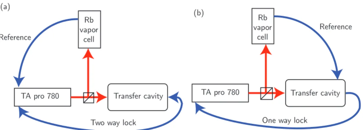
4.1 Transfer cavity . . . 36

4.2 Laser system and the path various optical beams . . . 37

4.3 Locking schemes for the master laser using transfer cavity 38 4.4 Transfer Cavity Stability . . . 39

4.5 Blue laser frequency stability . . . 39

4.6 Schematics of the acquisition system . . . 42

4.7 Experimental sequence . . . 43

5.1 An illustration of LVIS and the main chamber . . . 46

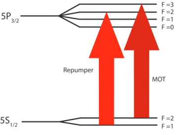
5.2 MOT excitation scheme . . . 47

5.3 LVIS and MOT traps along with the atomic beam . . . 48

5.4 Imaging setup. . . 50

5.5 The imaging scheme . . . 50

5.6 Temperature measurements . . . 51

6.2 Hanbury Brown Twiss type Interferometer to measure

In-tensity correlations . . . 55

6.3 Homodyne Tomography . . . 56

6.4 Measurement of electronic noise level . . . 57

6.5 Homodyne phase locking scheme . . . 58

6.6 Phase measurement in reflection . . . 60

6.7 Squeezing spectrum in transmission . . . 61

6.8 Phase measurements . . . 62

6.9 Phase dependent noise from laser . . . 62

6.10 Phase noise from the laser lock . . . 63

6.11 Intensity dependent phase noise from model . . . 63

6.12 Phase noise through cavity . . . 64

6.13 Dispersive non-linearities using Rydberg excitations . . . . 68

6.14 Resonant excitation scheme with experiment . . . 69

7.1 Main cavity setup . . . 72

7.2 Technical drawing of the cavity holder . . . 73

7.3 Cavity locking loop using PDH technique . . . 74

7.4 Cavity lock stability . . . 75

7.5 Cavity with incident and reflected fields . . . 76

7.6 Experimental Setup . . . 76

7.7 Configuration for small cloud preparation . . . 78

7.8 Experimental Sequence . . . 79

7.9 Images of atomic clouds during different stages . . . 80

7.10 Cooperativity measurement . . . 81

7.11 Probe intensity as seen by atoms . . . 82

7.12 A bird’s eye view of the blue cavity along with the viewports of the vacuum chamber . . . 83

7.13 Cross-section view of blue cavity along with optical beams 84 7.14 Blue inhomogeneous effects . . . 86

7.15 EIT measurements in linear regime . . . 87

7.16 Rydberg linewidth measurements . . . 88

7.17 Non-linearity using Rydberg S states . . . 89

7.18 Stark effect on Rydberg D states . . . 91

7.19 Transient measurements . . . 92

7.20 Probing long lived Rydberg D states . . . 93

7.21 Rydberg D-state nonlinearity . . . 94

8.1 Excitation scheme for photons . . . 98

8.2 g(2)_{(0) on resonant in reflection . . . . 99}

8.3 g(2)_{(0) in transmission . . . . 99}

8.4 Excitation scheme . . . 100

8.5 Intensity correlation measurement . . . 101

8.6 Phase dependent quadrature noise induced by Rydberg-Rydberg interactions . . . 102

8.7 EIT-induced quadrature noise at 700 kHz . . . 103

List of Figures

9.1 Rydberg blockade volume . . . 111

9.2 Cavity comparison . . . 112

9.3 Cavity waist size dependence on length. . . 113

9.4 Configuration of the bottom mirror . . . 114

9.5 Waist size of the TEM00 mode as a function of frequency spacing between the higher order TEM modes . . . 115

9.6 Different cavity modes excited . . . 116

9.7 Cavity linewidth measurement . . . 116

9.8 Cavity drifts . . . 117

9.9 EIT measurement . . . 119

9.10 Proposed excitation scheme in dispersive regime . . . 120

9.11 Statistics of transmitted light . . . 121

9.12 Phase gate . . . 122

9.13 Photonic controlled phase gate . . . 123

9.14 Fidelity of the gate . . . 124

A.1 Hyperfine structure of D2 transition . . . 132

C.1 Stark map of the 85 D state . . . 136

D.1 The Wigner function of a coherent state . . . 137

D.2 Cross section of a Wigner function of pure Fock states . . . 138

List of Tables

4.1 Summary of all required atomic transitions. . . 34

4.2 Summary of all lasers.. . . 35

4.3 Transfer cavity . . . 38

5.1 LVIS chamber parameters. . . 48

5.2 Main chamber parameters . . . 49

6.1 Comparision of the g(2) _{measurement and the Homodyne} detection . . . 56

7.1 Main cavity parameters. . . 72

7.2 Main cavity lock parameters . . . 75

7.3 Final sequence timings . . . 80

7.4 Blue cavity paramters . . . 82

7.5 Blue locking specifications . . . 85

9.1 Main cavity parameters. . . 117

A.1 Selected fundamental constants. . . 131

A.2 Properties of 87_{Rb atoms. . . . 132}

Preface and Overview

List of abbreviations used in this thesis

LVIS Low Velocity Intense source MOT Magneto Optical Trap

EIT Electromagnetically Induced Transparency AOM Acoustic Optic Modulator

EOM Electro Optic Modulator LO Local Oscillator

SPCM Single Photon Counting Module PDH Pound Drever Hall lock

PID Proportional-Integral-Derivative controller FALC Fast Analog Linewidth Control

PZT Piezo Transducer

UHV Ultra High Vacuum (< 10−8 _Torr)

DDS Direct Digital Synthesizers

Ti:Saph Titanium-doped Sapphire (Ti:𝐴𝑙2𝑂3)

IR Infrared

RF Radio frequency PD Photo diode

Chapter

1

Introduction

According to Moore’s law, the number of transistors per cm2 _{would increase}

expo-nentially by doubling every 1 to 2 years [1]. Soon enough we will reach a fundamental boundary where the storage of information can no longer be explained by classical laws [2]. The strange effects in the physics of individual quantum objects will start to play role in how the electrons behaves. Hence, it’s necessary to understand how we can take these effects into consideration and go beyond the classical systems. Quantum computation is a way of exploiting the special properties of the quantum world to speed up computational process. Richard Feynman speculated that quan-tum systems can be used to build advanced simulators [3]. This idea has attained a significant interest since Shor developed a quantum algorithm to factorize a large number (N) [4]. Shor’s quantum factorization method can run in polynomial time in log(N) whereas the best classical method (general number field sieve) scales ex-ponentially in log(N) [5]. The experimental realization of quantum simulators or computers has motivated many research groups. Numerous interesting algorithms have been proposed but their experimental implementation in large scales is still a long standing goal.

Quantum Computation

In computers, the information is stored in the form of zeros and ones known as bits. The smallest units of a quantum computing machine are known as quantum bits, also referred to as qubits [6]. Unlike classical bits, each qubit can exist in superposition states and qubits can be entangled with one another. This enables quantum computers to perform calculations in a vast Hilbert space at higher speed. These properties give quantum computers an unprecedented advantage over their classical counterpart.

A quantum computer cannot be built like a classical one as it requires a new technology which can enable us to store information in superposition states. There has been a considerable progress in the last decade to make quantum computation a reality. There are many quantum systems such as neutral or charged atoms, superconducting qubits, quantum dots etc., which have many characteristic traits to become a component of a quantum computer. Currently, it is possible to

en-gineer quantum states like Schrödinger cat states using optical systems [7,8] and microwave photons [9,10]. However, in most of these schemes realizing a system which has a strong isolation from environment and on demand ‘on/off’ control over interactions is a technical challenge. Some companies like ‘D-wave Systems’ claim they invented the first quantum computer, but they use “quantum annealing” for adjusting interactions to shape the final collective quantum state. Upto now this type of approach cannot be scaled up efficiently without overcoming environmental noise.

Modular quantum networks

Scaling up quantum systems without losing their coherence is an ambitious task. The conventional way of connecting every qubit to one another is likely to fail due to buildup of errors. Algorithms like quantum error correction require more qubits to correct for errors which in turn increases the complexity of the system. A promising solution is distributed quantum information processing or modular networks, where the quantum nodes are connected by networks of channels [11,12]. Instead of entangling all the qubits with one another, few qubits form a node which makes it easier to manage them [13]. Our group’s approach is to use cavity enhanced neutral atoms with photons as carriers. In Figure 1.1 cavity systems at nodes are connected to each other via channels like fiber optical links.

A

C

B

Figure 1.1: Modular computing: A quantum network of nodes A, B and C are connected by channels like fiber optic links. Each node consists of cavity systems. In distributed networks, nodes process information and perform quantum operations like quantum gates, etc.

Photons as flying qubits

For the past decade, optical fibers have dominated as information communication channels. Photons are robust against environmental noise which makes them ideal

Introduction

candidates for information transfer [14]. They can be transported with ease over long distances and can be incorporated into existing communication channels. Pho-tons are also relatively easy to produce using many systems like spontaneous para-metric down-conversion or cold atomic memories. Several existing methods such as Hanbury Brown and Twiss effect or homodyne tomography help us to easily characterize the quality of these photons [15,16].

In conventional optical fiber systems, it is common to use optical amplifiers to boost the signal to transport it over long distances. For quantum networks, a specific system, the quantum repeater, has been designed to counteract the decoher-ence effects introduced during transmission over long distances. One cannot simply detect or amplify the signal akin to classical communication. A quantum repeater system transports information without actually measuring it. The standard ap-proach involves a source of entangled photons and a quantum repeater node where logical operations take place. In order to project the signal state onto one of the entangled photon, a projective measurement operation is carried out between the signal photon and the other entangled one. In addition, by using an entanglement purification process between different nodes, photonic states can be transferred over long distances with high fidelity [17,18].

Quantum computation using photons

The main building blocks of quantum networks are non-classical states and coherent manipulation techniques. A gate operation is necessary for the realization of a full scale computational system [19]. One commonly used multi-bit gate is a controlled phase gate where one of the input bits acts as a control. The operations of a controlled phase gate are illustrated in Figure 1.2.

|s〉 |c〉 |c〉 |s’〉 |c〉|s〉 |c〉|s’〉

Input Output

Figure 1.2: Quantum Control Z gate: Control phase or Z gate is a two qubit gate where one of the input qubits acts as a control (|𝑐⟩). The other input qubit is represented as |𝑠⟩. The output state of the gate is the same as the input state except when both the signal and the control qubit are in state ‘1’, then it acquires a phase of 𝜋.

In 2001, Knill et. al. [20] proposed a scheme where single photons coupled with linear elements (like beam splitters, phase shifters) can be used for quantum information protocols. However its experimental implementation demands highly

efficient single photon sources and counters. In addition, they are inherently prob-abilistic [21]. Therefore, we resort to photon-photon nonlinearities for realization of quantum gates.

Since photons interact weakly with one another, it is a challenging task to ob-serve non-linearities at few photon level. To achieve deterministic quantum in-teractions, we need strongly non-linear systems [22,23]. For example, if we need an infrared photon wave packet (with a bandwidth of 1 MHz) to attain an optical phase shift of 𝜋 by propagating in a medium of length equal to Rayleigh range of the photon then the medium’s third order susceptibility(𝜒(3)_{) has to be greater than}

10−3V−2m2 [24]. But conventional optical medias exhibit extremely weak optical

susceptibilities and the phase shift obtained is twenty orders of magnitude lower than the desired value [24]. Strong Kerr non-linear effects can be realized by using resonant optical medias like cold atoms or trapped ions [25].

Cold atoms

Quantum optical non-linearities using atomic ensemble as an intermediary medium has gained a significant interest since the proposal by Jaksch et.al. [26]. Cold atoms have well established trapping techniques along with tremendous control over its states which makes them promising candidates for quantum computers. Information can be stored in ‘built-in’ internal states of atoms which possess long coherence times. In addition, it is possible to use optical lattices to scale up neutral atomic systems [27]. Dipole-dipole interactions between atoms can influence the properties of neighboring atoms and can give rise to collective cooperative behavior like super-radiance [28]. These interactions can be only observable in a very dense atomic ensembles like BEC, etc. Our main objective is to enhance these interactions to achieve quantum optical non-linearity in atomic clouds. Until now, the two main promising approaches to strong photon-photon interactions are Electromagnetically Induced Transparency (EIT) and cavity Quantum Electro-Dynamics (cQED) [29]. To enhance the optical non-linearity one can couple a two-level system to a high finesse optical cavity. The study of this strong coupling between the atoms and cavity is referred to as cQED. Many interesting results have been obtained using cavity QED systems since the demonstration of quantum state manipulation using microwave cQED [9,10].

Two level atomic media can exhibit strong non-linear response close to resonance, but the photons are lost by scattering. In 1990, Harris et al. proposed that by adding an additional coupling transition, the medium can be rendered transparent while enhancing the optical susceptibilities [30,31]. In addition, the group velocity of the light is strongly reduced which allows us to store light as polaritons [32]. The reported susceptibilities are still not sufficient to achieve a phase shift of 𝜋 at few photon level.

Our approach is to use long range dipole-dipole interactions between collective atomic excitations to achieve quantum optical non-linearities. In the next section, we present how one can tune the dipole-dipole interaction strength to achieve few photon non-linearities.

Introduction

Figure 1.3: Rydberg-Rydberg interaction energy shift vs Interatomic dis-tance: When an atom (b) is far from a Rydberg atom then it can be excited to a Rydberg level using resonant lasers. If an atom (a) moves closer then its energy levels are perturbed and it is no longer possible to excite it to Rydberg state. The minimum distance upto which a Rydberg atom can influence another is defined as Rydberg blockade radius (𝑟𝑏). A typical blockade radius is of the order of ∼ 5 𝜇m.

Strong photonic non-linearities via Rydberg EIT

The idea is to map the photons onto highly excited atomic states called Rydberg states and then use the long range dipole-dipole interactions between them to enable photon-photon interaction. The idea of using Rydberg atoms has generated sub-stantial interest since the proposal of non-classical state generation using the ‘dipole blockade’ mechanism in mesoscopic ensembles [22]. However, exciting them directly to Rydberg states using only optical light is inefficient because of their weak transi-tion dipole moments. In 2005, Friedler et. al. proposed exciting to Rydberg states using EIT, where a two photon excitation scheme is used to render the medium transparent [33]. Prior to this, most EIT experiments were carried out using a sec-ond ground state as metastable state. They showed that two photon pulses can be converted to dark state polaritons which interact via dipole-dipole interactions and acquire a phase shift of 𝜋 to realize a photonic gate. Moreover, Rydberg atoms in optical lattices can be used as a simulator for many body interaction systems [34]. Since then, a number of interesting experiments have been carried out to con-vert photonic excitations to Rydberg polaritons starting with the group of Charles Adams at University of Durham [35] during 2010-13. They demonstrated optical non-linear effects in classical regime using free-space atomic systems. More recently, non-linearities at quantum level have been demonstrated by creating a single pho-ton source [36], a photon blockade where only single photons are transmitted [37], photon bunching in dispersive regime [38]. A Rydberg based photon switch where a

Introduction

Thesis Layout

This thesis is a summary of the work carried out at the Institut d’Optique in an attempt to observe quantum optical non-linearities. We use a cold atomic cloud trapped in the mode of a low finesse optical cavity. This system has been chosen for its ability to combine the advantages of cavity and atomic cloud systems. This manuscript is organized in the following manner

∙ In part 1, we establish a standard notation for the computation of various relevant parameters of our system. We show why optical interactions induced by two level and three level non-interacting EIT systems is not sufficient to move to the quantum regine. We also introduce two models to explain Rydberg induced optical non-linearities in the classical regime.

∙ In part 2, we describe various parts of our experimental setup, and present the necessary lasers and hardware required to trap atoms. We conclude with various atomic cloud characterization methods.

∙ In part 3, we begin with various detection methods available on our setup and go on to present the Rydberg non-linearity measurements for S and D states. We also describe higher order correlation effects predicted for the mea-sured non-linearity. We conclude the chapter with second order correlation measurements using a Hanbury Brown Twiss setup and squeezing spectrum measurements using a homodyne setup.

∙ In part 4, we present how a new high finesse cavity with a small mode-waist designed to move towards the quantum regime. We describe the new cavity de-sign and its properties. We include details on how the new cavity is mounted and characterized on our setup. We present the recent EIT measurements along with some numerical calculations of squeezing spectrum expected with the new setup. We also present some theoretical ideas which could be imple-mented with the new setup, which would allow us to observe quantum optical non-linearities.

Part I

Chapter

2

Theoretical tools for Atom-Light

coupling

Contents

2.1 Light propagation in a dielectric medium . . . 11

2.2 Semi-classical approach of the light-atom system . . . 12

2.3 Quantum mechanical approach . . . 15

2.3.1 Optical Bloch equations . . . 16

2.3.2 Optical bistability using two level atoms . . . 18

2.4 Three level atoms . . . 20

2.4.1 Electromagnetically Induced Transparency. . . 21

2.4.2 Linear response . . . 22

2.4.3 Multilevel system . . . 23

2.5 Non-linearity . . . 24

In this chapter we will present the framework to describe our atom-cavity system. We will establish basic notions of light propagation through a cavity enhanced cold atomic media by deriving the expressions for susceptibility. We will show how to quantify the non-linearity arising from two-level and multi level atoms. Finally, we show why one needs to go beyond these systems to have quantum optical non-linearities.

2.1 Light propagation in a dielectric medium

Here we introduce expressions for a classical field propagating in a dielectric medium. The optical waves propagate through a dielectric medium by continuous absorption and re-emission of wave energy by atoms in the medium. This light-matter interac-tion can be quantified by defining a parameter called polarizability of the medium. It is related to the induced polarization ⃗𝑃 (⃗𝑟, 𝑡) by the propagating electromagnetic

wave ⃗𝐸(⃗𝑟, 𝑡) [49] ⃗ 𝑃 (⃗𝑟, 𝑡) = 𝑡 ∫︁ −∞ 𝑑𝑡′𝛼1(𝑡 − 𝑡′) ⃗𝐸(⃗𝑟, 𝑡′)𝑑𝑡′+ 𝑡 ∫︁ −∞ 𝑡 ∫︁ −∞ 𝑑𝑡′′𝛼2(𝑡 − 𝑡′, 𝑡 − 𝑡′′) ⃗𝐸(⃗𝑟, 𝑡′) ⃗𝐸(⃗𝑟, 𝑡′′) + ... (2.1) Where 𝛼𝑖 is the polarizability of the medium of order i. This induced polarization

in turn affects both the phase and the amplitude of the propagating electromag-netic waves. If we expand the incoming field in the frequency domain, then the polarization can be written as

𝑃 (𝜔) = 𝜀0𝜒(𝜔)𝐸(𝜔) (2.2)

𝜒(𝜔) = 𝜒1(𝜔) + 𝜒2(𝜔)𝐸(𝜔) + 𝜒3(𝜔 = 𝜔1+ 𝜔2)𝐸1(𝜔1)𝐸2(𝜔2)... (2.3)

The real part of the susceptibility contributes to the dispersion of light, and the imaginary part to the absorption of light. From the above expression we can evaluate the effect of matter on light using the the expression 𝑛 = √1 + 𝜒. Most materials and gases exhibit centro-symmetry and it can be shown that the second order term vanishes in these media. In linear systems, one can neglect all the higher order terms and the susceptibility term is independent of the field strength. In non-linear systems, the third order term is the lowest contributing one and the susceptibility depends on the incoming field’s intensity. In the following sections we will describe how one can evaluate the susceptibility term in atomic systems.

2.2 Semi-classical approach of the light-atom

sys-tem

A monochromatic wave incident on an atomic medium close to the resonance of two-levels can be described by a semi-classical approach, where the atoms are considered as two level quantum systems. We denote the two levels of the atom as g (ground state) and e (excited state). The energy difference between the levels is represented by 𝐸𝑒 − 𝐸𝑔 = ~𝜔𝑔𝑒. We introduce atomic operators that are denoted by ˆ𝜎

(𝑛) 𝑘𝑙 =

|𝑘⟩⟨𝑙| for atom 𝑛. The atomic Hamiltonian for atom ‘n’ can then be denoted by ℋ(𝑛)𝑎 = ~𝜔𝑔𝑒(ˆ𝜎

(𝑛)

𝑒𝑔 𝜎ˆ(𝑛)𝑔𝑒 ). The light-atom system can be described by evaluating

ℋ𝑠 = ℋ𝑎+ ℋ𝑖 (2.4)

As we treat light classically ( ⃗𝐸(𝜔) = ℰ0⃗𝑢 (𝑒𝑖𝜔𝑡+ 𝑒−𝑖𝜔𝑡)), we consider that the only

role of light is to create an interaction potential. An atom driven close to the resonance of an optical transition can be considered as an oscillating dipole. The transition moment operator of the atom ’n’ for |𝑔⟩ → |𝑒⟩ is given by

ˆ ⃗

𝑑(𝑛)= 𝑑0⃗𝑢(ˆ𝜎(𝑛)𝑔𝑒 + ˆ𝜎 (𝑛)

2.2. Semi-classical approach of the light-atom system

I

₀

I

ω

ω

χ

|g〉

|e〉

Figure 2.1: Two-level excitation scheme: Each atom is considered as a two-level system with ground state ‘g’ and excited state ‘e’. An optical beam with intensity I0

is incident on the atomic media with frequency 𝜔, and we denote the susceptibility of the atoms as 𝜒. The energy difference between the two levels is denoted by 𝜔𝑔𝑒.

By using the rotating wave approximation1_{, one can neglect the rapidly}

oscil-lating terms and rewrite the interaction Hamiltonian as ℋ𝑖𝑛𝑡=∑︀_𝑛−𝐷⃗ˆ(𝑛). ⃗𝐸(𝑟𝑎) =

∑︀

𝑛𝑑0ℰ0

(︁

𝑒−𝑖𝜔𝑡𝜎ˆ𝑔𝑒(𝑛)+ 𝑒𝑖𝜔𝑡𝜎ˆ(𝑛)𝑒𝑔 )︁. The total Hamiltonian of the system can be

ex-pressed as ˆ ℋ𝑠= ~∆𝑒 𝑁 ∑︁ 𝑛 ˆ 𝜎_𝑒𝑒(𝑛)+∑︁ 𝑛 ~Ω [︁ 𝑒−𝑖𝜔𝑡𝜎ˆ_𝑔𝑒(𝑛)+ 𝑒𝑖𝜔𝑡𝜎ˆ_𝑒𝑔(𝑛)]︁ (2.6) where Ω = −(𝑑0ℰ0)/~, 𝑁 is total number of atoms and ∆𝑒 = 𝜔 − 𝜔𝑔𝑒. One can then

use Heisenberg equations to evaluate the evolution of any operator ˆ𝐴 using [51]. 𝑑 𝑑𝑡 ˆ 𝐴 = 𝑖 ~ [ ˆℋ𝑠, ˆ𝐴] − 𝛾_𝐴^𝐴 + 𝐹ˆ 𝑎 (2.7)

where 𝛾𝑒 is the decay rate of the excited state and 𝐹𝑎is the Langevin noise operator

associated with the operator ˆ𝐴. Using the steady state approximation, we obtain the following expression for the average value of the coherence term (ˆ𝜎𝑔𝑒)

⟨︀ ˆ𝜎(𝑛)_𝑔𝑒 ⟩︀ = 𝑖Ω( ⟨ ˆ 𝜎𝑒𝑒(𝑛) ⟩ −⟨𝜎ˆ(𝑛)𝑔𝑔 ⟩ ) 2(𝛾𝑒+ 𝑖∆𝑒) = − 𝑖Ω 2(𝛾𝑒+ 𝑖∆𝑒) 1 (1 + _2(𝛾2Ω2 𝑒+Δ2𝑒)) ; = Ω 2 ∆𝑒− 𝑖𝛾𝑒 𝛾2 𝑒 + ∆2𝑒+ Ω2/2 (2.8) where 𝛾𝑒 = 𝑑2 0𝑘3

6𝜋𝜀0~ is half of the natural linewidth of the excited state.

We can define an average coherence term using ˆ𝜎𝑔𝑒 = _𝑁1

∑︀

𝑛𝜎ˆ (𝑛)

𝑔𝑒 . If the medium

has a uniform density 𝜌 then one can estimate the induced polarization density 𝑃 (𝜔) = 𝜌⟨ ˆ𝐷⟩ = 𝜌𝑑0⟨︀ ˆ𝜎𝑔𝑒𝑒−𝑖𝜔𝑡+ ˆ𝜎𝑒𝑔𝑒𝑖𝜔𝑡⟩︀ =

1

2𝜀𝑜ℰ0(︀𝜒(𝜔)𝑒

−𝑖𝜔𝑡

+ 𝜒*(𝜔)𝑒𝑖𝜔𝑡)︀ (2.9) which gives the following expression for the atomic susceptibility

𝜒(𝜔) = 𝜌𝑑 2 0 ~𝜀0 ⟨ˆ𝜎𝑔𝑒⟩ Ω/2 = − 𝛼0𝛾𝑒 𝑘 ⟨ˆ𝜎𝑔𝑒⟩ Ω/2 (2.10)

1_{Complete derivation can be found in many standard textbooks, for example [50]}

In the above equation we used the standard expressions for resonant optical cross-section for a two-level atom 𝜎eff = 3𝜆

2

2𝜋 and 𝛼0 = 𝜌𝜎eff [52]. The optical susceptibility

is proportional to the term ⟨ˆ𝜎𝑔𝑒⟩ /Ω ∝ (∆𝑒− 𝑖𝛾𝑒)/2(𝛾𝑒2+ ∆2𝑒) in the weak feeding

approximation (𝛾2

𝑒 + ∆2𝑒 ≫ Ω2). It is worth noting that the susceptibility doesn’t

depend on input intensity, hence the response of the system is linear in this regime.

Classical field in an optical cavity

We consider a linear cavity of length ‘L’ with an enclosed atomic medium. We represent the reflectivities of its mirrors by 𝑅1 = 1 − 𝑇1 ≈ 1 and 𝑅2 = 1 − 𝑇2 and

its resonant frequency by 𝜔𝑐. The normalized transmission of the cavity is given by 𝑇1𝑇2

|(1−√𝑅1𝑅2𝑒𝑖Δ𝑐/𝜔𝑓)|2 where 𝜔𝑓

= _𝐿𝑐 and the cavity detuning ∆𝑐= 𝜔 − 𝜔𝑐.

Free Space Cavity -20 -10 0 10 20 0.0 0.2 0.4 0.6 0.8 1.0 Probe detuning in _e Transmission Free Space Cavity T₁ T₂

Figure 2.2: Comparison of free space and cavity transmission. On the left: We observe the transmission of a probe beam close to atomic resonance. We assume the cavity to be resonant with the atoms and the transmission coefficients of input and output mirrors are 𝑇1 and 𝑇2 respectively. On the right: The

nor-malized transmission as a function of probe detuning when scanned around the atomic resonance. The blue line denotes the transmission of atoms in free space, whereas the red line represents the transmission through a cavity finesse of 100 and a cooperativity of 8.

If we have a medium of length 𝑙 inside the cavity with refractive index 𝑛 = √

1 + 𝜒 ≈ 1+𝜒/2, then the light acquires a complex phase 𝑒𝑖𝜋_𝜆𝜒𝑙per single pass. The

transmission through the cavity in this case can be written as 𝑇1𝑇2

|(1−√𝑅1𝑅2𝑒𝑖Δ𝑐/𝜔𝑓𝑒𝑖 2𝜋𝜆𝜒𝑙)|2

which can be approximated to 𝑇 = 𝐼𝑡 𝐼𝑖 ≈ 𝑇1𝑇2 (1 −√𝑅1𝑅2+ 2𝜋_𝜆 ℑ(𝜒)𝑙)2+ 𝑅1𝑅2sin2(∆𝑐/𝜔𝑓 + 2𝜋ℜ(𝜒)/𝜆𝑙) ≈ 4𝑇1/𝑇2 (1 + 4𝜋 𝑇2𝜆ℑ(𝜒)𝑙) 2_{+ (∆} 𝑐/𝛾𝑐+ 4𝜋ℜ(𝜒)/𝑇2𝜆𝑙)2 (2.11) where 𝛾𝑐 = 𝑇2𝜔𝑓/2 by using 𝑅1, 𝑅2 ≈ 1 and |𝜒| ≪ 𝜆/2𝜋𝑙. In the case of atoms

2.3. Quantum mechanical approach rewritten as 𝑇 = 𝑇0 (︁ 1 − 4𝛼0𝑙𝛾𝑒 𝑇2Ω ℑ(⟨ˆ𝜎𝑔𝑒⟩) )︁2 +(︁Δ𝑐 𝛾𝑐 − 4𝛼0𝑙𝛾𝑒 𝑇2Ω ℜ(⟨ˆ𝜎𝑔𝑒⟩) )︁2 = 𝑇0 (︁ 1 − _Ω/2𝛾2𝐶 𝑒ℑ(⟨ˆ𝜎𝑔𝑒⟩) )︁2 +(︁Δ𝑐 𝛾𝑐 − 2𝐶 Ω/2𝛾𝑒ℜ(⟨ˆ𝜎𝑔𝑒⟩) )︁2 = 𝑇0 (︁ 1 − 2𝐶 1+Δ2 𝑒/𝛾𝑒2+Ω2/2𝛾𝑒2 )︁2 +(︁Δ𝑐 𝛾𝑐 − 2𝐶Δ𝑒/𝛾𝑒 1+Δ2 𝑒/𝛾2𝑒+Ω2/2𝛾𝑒2 )︁2 (2.12) where 𝑇0 = 4𝑇1/𝑇2 and 𝐶 = 𝛼_𝑇0𝑙

2 is the ratio of the absorption of the media (also

known as optical depth) to the transmission of the lossy mirror. The term C is commonly referred to as the cooperativity of the medium and corresponds to a collective phenomena exhibited by the atoms.

As shown in Figure 2.2, the cavity transmission contains two normal modes when the detuning of the probe light is scanned around the atomic resonance. The position of the modes corresponds to those detunings for which the second term in the denominator goes to zero. In the weak feeding approximation, for large cooperativities the modes are separated by √8𝐶𝛾𝑐𝛾𝑒 when the cavity is resonant

with the atoms.

2.3 Quantum mechanical approach

In order to more accurately describe the system evolution we use a fully quantum mechanical approach to describe the light-atom coupling. We quantize the electro-magnetic field in the cavity mode in the Schrödinger picture. By using the second quantization, we can describe the Hamiltonian of the single mode light field by

ℋ𝑙 = ~𝜔𝑐 (︂ ˆ 𝑎†ˆ𝑎 + 1 2 )︂ (2.13) where 𝜔𝑐 is the cavity resonance frequency. We restrict ourselves to excitations

only in the fundamental mode of the cavity. We can then write the quantized electromagnetic field operator in a cavity by using the boundary conditions for a cavity placed along the z axis [53]

ˆ

𝐸(𝑥, 𝑦, 𝑧) = ⃗ℰ(𝑥, 𝑦, 𝑧)[︀ˆ𝑎𝑒𝑖𝑘𝑧 _{+ ˆ𝑎}†

𝑒−𝑖𝑘𝑧]︀

= ⃗ℰ(𝑥, 𝑦, 𝑧)(︀cos(𝑘𝑧) [︀ˆ𝑎 + ˆ𝑎†_{]︀ + 𝑖 sin(𝑘𝑧) [︀ˆ𝑎 − ˆ𝑎}†]︀)︀

(2.14) where 𝑘 = 𝜔𝑐/𝑐. We also assume that all the atoms are restricted within the

Rayleigh range of the cavity mode, and hence the waist is assumed to be constant 𝜔(𝑧) ≈ 𝜔0. The electric field term can be written as ⃗ℰ(𝑥, 𝑦, 𝑧) = ℰ0⃗𝑢𝑒

−𝑥2+𝑦2 2𝑤2 0 , where ℰ0 = √︁ ~𝜔𝑐

2𝑉 𝜀0 is the electric field per photon and the mode volume is 𝑉 =

∫︀ cos2_{(𝑘𝑧)𝑒}−

𝑥2+𝑦2 2𝑤2_{0 𝑑}3_𝑟 .

Our system is composed of N atoms interacting with a single cavity mode. One can describe such a system using the Dicke model [28], where the atomic dipoles are coherently interacting with the electromagnetic field. The cavity is pumped with a coherent feeding rate 𝛼. Here we work in the open cavity limit (𝜆 ≪ 𝐿), where the spontaneous emission rate (𝛾𝑒) for an atom is close to its value in free space. The

total Hamiltonian is given by ˆ ℋ𝑠 = ˆℋ𝑙+ ˆℋ𝑎+ ˆℋ𝑖𝑛𝑡+ ˆℋ𝑓 = ~∆𝑐ˆ𝑎†ˆ𝑎 + ∑︁ 𝑛 ~∆𝑒𝜎ˆ𝑒𝑒(𝑛)− ∑︁ 𝑛 ~𝑔(𝑟𝑛) [︁ ˆ 𝑎ˆ𝜎_𝑔𝑒(𝑛)+ ˆ𝑎†𝜎ˆ(𝑛)_𝑒𝑔 ]︁_{+ ~𝛼(ˆ𝑎 + ˆ𝑎}†) (2.15) In the above expression, the position dependent atom-light coupling term is given by 𝑔(𝑟𝑛) = 𝑔0𝒮(𝑟𝑛) where 𝑔0 = 𝑑0

√︁ _𝜔

𝑐

2~𝜀0𝑉 is the vacuum Rabi frequency term and

the function 𝒮(𝑟𝑛) = cos(𝑘𝑧)𝑒 −𝑥2+𝑦2

2𝑤2₀ depends on position of each atom 𝑟

𝑛.

2.3.1 Optical Bloch equations

The dynamics of the system can be described by using the density matrix formalism (Schrödinger picture) or by Heisenberg-Langevin equations (Heisenberg picture). As our system exhibits dissipation, it is easier to describe using master equation in the Lindblad form. We must take into account both the dissipation of the cavity (ˆ𝑎) and atoms ˆ𝜎𝑔𝑒 to establish the evolution of the system. The evolution of the density

matrix(𝜌𝑠) can be expressed using Liouvillian terms (ℒ( ˆ𝐴)𝜌𝑠) in the following form

˙ˆ 𝜌𝑠 = − 𝑖 ~ [︁ ˆ_{ℋ𝑠, ˆ𝜌𝑠}]︁ − 𝛾𝑐(ˆ𝑎†ˆ𝑎 ˆ𝜌𝑠+ ˆ𝜌𝑠ˆ𝑎†𝑎 − 2ˆˆ 𝑎 ˆ𝜌𝑠ˆ𝑎†) − 𝛾𝑒(ˆ𝜎𝑔𝑒𝜎ˆ𝑒𝑔𝜌ˆ𝑠+ ˆ𝜌𝑠𝜎ˆ𝑔𝑒𝜎ˆ𝑒𝑔− 2ˆ𝜎𝑒𝑔𝜌ˆ𝑠𝜎ˆ𝑔𝑒) (2.16)

From the above master equation we can extract the expectation values of the operators using the expression ⟨ ˆ𝐴⟩ = Tr( ˆ𝐴 ˆ𝜌𝑠). The evolution of operators can

be evaluated from 𝑑

𝑑𝑡⟨ ˆ𝐴⟩ = Tr( ˙ˆ𝜌 ˆ𝐴) which gives the Heisenberg equations for the

operators 𝑑

𝑑𝑡⟨ ˆ𝐴⟩ = 𝑖

~⟨[ ˆℋ𝑠, ˆ𝐴]⟩ − 𝛾⟨ ^𝐴⟩

ˆ

𝐴 [51]. The evolution of the intracavity field and the coherence terms can be calculated using

𝑑 𝑑𝑡⟨ˆ𝑎⟩ = (𝑖∆𝑐− 𝛾𝑐)⟨ˆ𝑎⟩ + ∑︁ 𝑛 𝑔(𝑟𝑛)⟨ˆ𝜎(𝑛)𝑔𝑒 ⟩ − 𝑖𝛼 (2.17) 𝑑 𝑑𝑡⟨ˆ𝜎 (𝑛) 𝑔𝑒 ⟩ = (𝑖∆𝑒− 𝛾𝑒)⟨ˆ𝜎(𝑛)𝑔𝑒 ⟩ + 𝑖𝑔(𝑟𝑛)⟨ˆ𝑎(ˆ𝜎𝑒𝑒(𝑛)− ˆ𝜎 (𝑛) 𝑔𝑔 )⟩ (2.18)

where the term 𝛼 denotes the feeding rate into the cavity. In the steady state condition, we observe that

⟨ˆ𝜎𝑔𝑒(𝑛)⟩ ⟨ˆ𝑎⟩ = 𝑖𝑔(𝑟𝑛) (∆𝑒+ 𝑖𝛾𝑒) 𝑓 (⟨ˆ𝑎⟩2) (2.19) ⟨ˆ𝑎⟩ = _(︁ 𝛼 ∆𝑐+ 𝑖𝛾𝑐− 𝑖 ∑︀ 𝑛𝑔(𝑟𝑛) ⟨^𝜎𝑔𝑒(𝑛)⟩ ⟨^𝑎⟩ )︁ = 𝛼 (︁ ∆𝑐+ 𝑖𝛾𝑐+∑︀_𝑛𝑔 2_(𝑟 𝑛) 𝛾𝑐𝛾𝑒 𝜒𝑛 )︁ (2.20) where 𝜒𝑛 = _𝑔(𝑟𝛾𝑒_𝑛) ⟨^𝜎(𝑛)𝑔𝑒 ⟩

⟨^𝑎⟩ is the susceptibility of each atom n. In a linear regime the

function f(⟨ˆ𝑎⟩2_{)is a constant and can be shown to be equivalent to the semi-classical}

2.3. Quantum mechanical approach Cavity transmission

The normalized transmission of the cavity is proportional to the intracavity inten-sity. In steady state, for a weak feeding rate the normalized cavity transmission can be evaluated from 𝑇 = ⟨ˆ𝑎⟩ 2_𝛾2 𝑐 𝛼2 = 𝑇0 (︁ 1 + ℑ(∑︀ 𝑛 𝑔2_(𝑟 𝑛) 𝛾𝑐𝛾𝑒 𝜒𝑛) )︁2 +(︁Δ𝑐 𝛾𝑐 + ℜ( ∑︀ 𝑛 𝑔2_(𝑟 𝑛) 𝛾𝑐𝛾𝐸 𝜒𝑛) )︁2 (2.21) ≈ 𝑇0 (︁ 1 −_1+Δ2𝐶2 𝑒/𝛾𝑒2 )︁2 +(︁Δ𝑐 𝛾𝑐 − 2𝐶Δ𝑒/𝛾𝑒 1+Δ2 𝑒/𝛾2𝑒 )︁2 (2.22)

where T0 is a proportionality constant and 𝐶 = ∑︀_𝑛 𝑔

2_(𝑟 𝑛)

2𝛾𝑐𝛾𝑒. It must be noted here

that the cooperativity parameter is equivalent to the one we derived in section : 2.2. It is an important figure of merit across various systems to quantify the coherent atom-light coupling. It is the ratio of the square of the coherent coupling to the product of the dissipation rates (cavity and atoms). The effective volume over an atomic medium of length 𝑙 can be evaluated by

𝑉 = ∫︀ 𝑑 3_{⃗𝑟⟨𝐸⃗}ˆ +(⃗𝑟)2⟩ ⟨𝐸⃗ˆ𝑚𝑎𝑥(⃗𝑟)2⟩ = ∫︁ ∫︁ ∫︁ 𝑑𝑥𝑑𝑦𝑑𝑧 cos2(𝑘𝑧)𝑒−2 𝑥2+𝑦2 𝜔2 0 = 𝜋 4𝐿𝜔 2 0 where the_𝐸⃗ˆ

+ is one of the propagating field components. If we assume the medium

has a uniform density 𝜌 then we can write ∑︀𝑛𝑔 2_(𝑟

𝑛) = 𝑔20𝜌𝜋𝑙𝜔20/4. Using the

expressions for 𝑔0, 𝛾𝑐, 𝛾𝑒, we can write cooperativity as 𝐶 = 𝑁

′ 𝑇1 3𝜆2 2𝜋𝜔2 0 where 𝑁 ′ ₌ 𝜌𝜋𝑙𝜔2

0/4 is the effective number of atoms coupled to the cavity.

-20 -10 0 10 20 Probe detuning ine 0.0 0.2 0.4 0.6 0.8 1.0 Tran smission Empty cavity C = 1 C = 2 C = 5 5 10 15 20 25 Probe detuning ine 0.0 0.2 0.4 0.6 0.8 1.0 Tran smission 30 0 Empty cavity C = 5 C = 10 C = 20 (a) (b)

Figure 2.3: Cooperativity measurement in absorptive and dispersive regime: The normalized cavity transmission versus probe detuning normalized to 𝛾𝑒 for a cavity with a decay rate 𝛾𝑐 = 3.3𝛾𝑒 (a) When the cavity is on

reso-nance with atoms the cavity transmission is split into two normal modes where the splitting is given by √8𝐶𝛾𝑐𝛾𝑒. (b) When the cavity is detuned from the resonance

of the atoms by ∆𝑒 = 15𝛾𝑒. The cavity transmission curve is shifted with a shift

proportional to the cooperativity.

To increase the cooperativity one needs to have a very high atomic density or a very high finesse cavity. In this thesis, we are going to concentrate on scenarios where the atom-light coupling 𝑔0 ≪ 𝛾𝑐, 𝛾𝑒 and

√

𝑁 𝑔0 > 𝛾𝑐, 𝛾𝑒.

2.3.2 Optical bistability using two level atoms

Optical non-linearity has acquired tremendous interest since the prediction of op-tical bistability in resonator systems with non-linear media in the 1970s and has been well studied by many groups [54–56]. Optical bistability or multistability is the presence of more than one possible value for transmission for a given input intensity. This phenomenon can be observed only when the imaginary part or the real part of the susceptibility is a function of the intensity. This phenomena can be used to create an optical switch where one can alternate between two stable points deterministically [51,57]. 8 6 4 0 10 2 15 20 25 30 35 40 X Y C = 3.5 C = 5 C = 4.3 C = 3.9

Figure 2.4: Absorptive non-linearity: The transmitted light (X) is plotted as a function of incident light (Y). We can see that for cooperativities higher than 4 there is a range of input intensities where the output light is multivalued.

Until now we have dealt with the situation where the susceptibility doesn’t depend on the intensity of the incident light. It is a valid approximation for weak intensities, where the excited level population is not saturated. As soon as we reach a regime where Ω2 _{∼ 𝛾}2

𝑒 + ∆2𝑒 then the susceptibility depends on the intracavity

field and vice versa.

We will show how the bistable behavior is originated in absorptive and disper-sive regimes. The incident and transmitted light are normalized using saturation intensity (𝐼𝑠𝑎𝑡) and expressed as 𝑋 = _𝑇2𝐼_𝐼𝑡_𝑠𝑎𝑡 = Ω

2

2𝛾2

𝑒 and 𝑌 =

𝐼𝑖

𝐼𝑠𝑎𝑡 [57,58]. We can

rewrite the stationary transmission functions of the cavity as 𝑋 = 𝑌 [︃ (︂ 1 − 2𝐶ℑ⟨ˆ𝜎𝑔𝑒⟩ Ω/2𝛾𝑒 )︂2 +(︂ ∆𝑐 𝛾𝑐 − 2𝐶ℜ⟨ˆ𝜎𝑔𝑒⟩ Ω/_2𝛾 𝑒 )︂2]︃−1 (2.23) where the term ⟨^𝜎𝑔𝑒⟩

Ω/2𝛾𝑒 is a function of 𝑋. If both the cavity and the atoms are on

2.3. Quantum mechanical approach transmission from 𝑌 = 𝑋 [︃ (︂ 1 + 2𝐶 1 + 𝑋 )︂2]︃ (2.24) The system can exhibit bistability when the cooperativity 𝐶 > 4 as shown in Figure

2.4. X Y 1 2 3 4 5 6 7 1 2 3 4 X  4 2 0 2 4 6 8 10 0.1 0.2 0.3 0.4 0.5 0 (b) (a)

Figure 2.5: Dispersive non-linearity: (a) The transmitted light vs incident in-tensity when 𝐴 = 1 and 𝐵 = 3 (b) Transmitted light vs the detuning of the probe from the cavity in a linear case when 𝑋 = 0.1 and non-linear when 𝑋 = 4.

On the contrary, if the detunings are much larger than the incident probe in-tensity (∆ ≫ Ω), then we are in the dispersive regime.

In the latter case the transmission function can be simplified to the following expression when ∆𝑒 ≫ 1and ∆𝑒 ≫ Δ_𝛾𝑐

𝑐 𝑋 = 𝑌 1 + (𝜃 − 2𝐶ℜ𝑓 (𝑋))2 (2.25) ≈ 𝑌 1 + (𝜃 −2𝐶_Δ 𝑒 + 2𝐶 Δ3 𝑒𝑋) 2 (2.26) where we replaced Δ𝑐

𝛾𝑐 by 𝜃. The above expression is in the form of 𝑌 = 𝑋(1 +

(𝐵 − 𝐴𝑋)2_{) where 𝐴 =} 2𝐶 Δ3

𝑒 and 𝐵 =

2𝐶

Δ𝑒 − 𝜃. It has more than one solution when

3𝐴2_𝑋2_{+ −4𝐴𝐵𝑋 + 𝐵}2_{+ 1 = 0}. It exhibits bistability when the term B is greater

than√3. In Figure 2.5(a) we see how the transmitted light varies with the incident probe intensity when 𝐵 = 3 and 𝐴 = 1.

In both cases of absorptive or dispersive bistability one needs to have X > 1 which corresponds to an intracavity intensity comparable to 𝐼𝑠𝑎𝑡. To achieve strong

non-linearity for few photons, one needs to have a small mode volume and large cavity bandwidth. This can be achievable in the cavity-QED, regime but for our cavity atomic system where the mode-waist is of the order of 10 - 100 microns and cavity decay rate of tens of MHz, one needs few thousands of photons to reach non-linear regimes.

2.4 Three level atoms

In order to further enhance the optical non-linearities one must move to multi-level systems where phenomena like Electromagnetically Induced Transparency allows us to move closer to resonance, without losing photons by scattering [30,59]. In addi-tion to the attenuated absorpaddi-tion window, the steep dispersion curve increases the effective interaction time between the probe pulses and atoms [60,61]. In the past two decades many groups have attempted, both theoretically and experimentally to lower the threshold to reach quantum regime [62–64].



,

Ω

_p





_s

,

Ω

_s

Δ

_s



|g〉

|e〉

|s〉





Ω

_p

Ω

_s

(a)

(b)

Figure 2.6: Illustration of the excitation scheme for three level atoms in a cavity: (a) The atoms are enclosed in a cavity with the probe coupled to the fundamental mode of the cavity and the control field incident from the side. (b) The three level excitation scheme is presented here along with the probe and the control fields.

In this section we will describe the optical response of three level atoms in a cavity. Consider an atom with a ground state (g), intermediate state (e), and a metastable state (s) separated by 𝜔𝑔𝑒 and 𝜔𝑒𝑠 respectively. The two atomic

tran-sitions |𝑔⟩ → |𝑒⟩ and |𝑒⟩ → |𝑠⟩ are driven by a probe beam at 𝜔 and a control coherent beam at 𝜔𝑠 respectively. The detunings of probe and control beam are

denoted by ∆𝑒= 𝜔 − 𝜔𝑔𝑒, ∆𝑠 = 𝜔𝑠+ 𝜔 − 𝜔𝑔𝑠. The additional Hamiltonian term for

three level atoms is ˆ ℋ𝑠 = −∆𝑠 ∑︁ 𝑛 ˆ 𝜎_𝑠𝑠(𝑛)+ Ω𝑠 2 ∑︁ 𝑛 (ˆ𝜎_𝑠𝑒(𝑛)+ ˆ𝜎_𝑒𝑠(𝑛)) (2.27)

Here we introduce a complex detuning term 𝐷𝑖 = ∆𝑖 + 𝑖𝛾𝑖. The optical Bloch

2.4. Three level atoms feeding rate of 𝛼 are

⟨ˆ𝑎⟩ = 1 𝐷𝑐 (𝑔∑︁ 𝑛 ⟨ˆ𝜎(𝑛)_𝑔𝑒 ⟩ + 𝛼) ⟨ˆ𝜎_𝑔𝑒(𝑛)⟩ = 1 𝐷𝑒 (︂ Ω𝑠 2 ⟨ˆ𝜎 (𝑛) 𝑔𝑠 ⟩ − 𝑔⟨ˆ𝑎(ˆ𝜎 (𝑛) 𝑒𝑒 − ˆ𝜎 (𝑛) 𝑔𝑔 )⟩ )︂ ⟨ˆ𝜎_𝑔𝑠(𝑛)⟩ = 1 𝐷𝑠 (︂ Ω𝑠 2 ⟨ˆ𝜎 (𝑛) 𝑔𝑒 ⟩ )︂ (2.28) From these equations we obtain the optical response of the system. In the next subsection we show some interesting effects which arise with three level system.

2.4.1 Electromagnetically Induced Transparency

In order to have a strong two level non-linear susceptibility one needs to move closer to resonance but the medium becomes opaque due to strong scattering by atoms. One way to circumvent this problem is by using Electromagnetically Induced Transparency, otherwise known as EIT. As the name indicates, the medium attains a narrow transparency band in the absorption spectrum and the dispersion spectra exhibits a steep slope when excited in certain conditions. Since the first observation of EIT [65], many groups have performed interesting experiments such as slow light [61], lasing without inversion [66], etc.

-15 -10 0 10 15 Probe detuning in e 5 5 0.0 0.2 0.4 0.6 0.8 1.0 Im( σ/Ω) Ωs = 5 Ωs = 0 - 20 - 10 0 10 20 -0.4 -0.2 0.0 0.2 0.4 Probe detuning in_e Re( σ/Ω) Ωs = 5 Ωs = 0 (a) (b) _e _e

Figure 2.7: Comparision of susceptibility of two level (red) and three level systems (blue): We assume that the linewidth 𝛾𝑠 = 0.1𝛾𝑒 (a) The real part of

the susceptibility shows the dispersion spectra. It shows a sharp response for the medium at zero detuning. (b) The absorption peak at resonance splits into two peaks creating a transparency window.

To understand how the transparency works, lets consider a system of three level atoms which are weakly driven (Ω𝑝 ≪ Ω𝑠, 𝛾𝑒) and all the transitions are resonant

(∆𝑖 = 0 for i = 𝑒, 𝑠, 𝑐 ) then the eigenstates of the system are (|𝑠⟩ ± |𝑒⟩)/

√ 2 and |𝑔⟩. The probe couples to the ±|𝑒⟩ components of the two eigenstates, which have equal magnitude and opposite sign. Hence it leads to destructive interference of both excitation pathways and therefore diminished absorption [30,59].

Free Space

Cavity

-20

-10

0

10

20

0.0

0.2

0.4

0.6

0.8

1.0

Probe detuning in 

Transmission

Figure 2.8: Electromagnetically induced transparency curves in the pres-ence and the abspres-ence of the cavity. The transmission of the system is plotted with respect to probe detuning normalized to 𝛾𝑒. We have assumed a low finesse

(100) one-sided cavity. The frequency of the probe beam is sweeped around the resonance and the control beam is incident on resonance with the secondary tran-sition (∆𝑠= 0). The value of control field Rabi frequency is assumed to be 2𝛾𝑒 and

the linewidth it taken to be 𝛾𝑠 = 0.06𝛾𝑒.

2.4.2 Linear response

The response of three level atoms can be simplified using the Bloch equation under weak feeding approximation and assuming all the atoms have equal coupling. If we neglect the atomic excitation (⟨ˆ𝜎(𝑛)

𝑒𝑒 − ˆ𝜎(𝑛)𝑔𝑔 ⟩ ≪ 1) then the coherence term for any

atom n is ⟨ˆ𝜎_𝑔𝑒(𝑛)⟩ ≈ 1 𝐷𝑒 (︂ Ω𝑠 2 ⟨ˆ𝜎 (𝑛) 𝑔𝑠 ⟩ + 𝑔⟨ˆ𝑎⟩ )︂ = 𝑔𝛼 ˜ 𝐷𝑒𝐷𝑐− ∑︀ 𝑛𝑔2 = 𝑔𝛼 ˜ 𝐷𝑒𝐷𝑐− 2𝛾𝑒𝛾𝑐𝐶 (2.29) The above expression is the same as two level susceptibility except that the term 𝐷𝑒 is replaced by ˜𝐷𝑒 = ∆𝑒− Ω

2 𝑠

4𝐷𝑠.

One can obtain an analytical expression to the transmission in steady state: 𝑇 = ⃒ ⃒ ⃒ ⃒ ⃒ 𝛾𝑐𝐷˜𝑒 ˜ 𝐷𝑒𝐷𝑐− 2𝛾𝑐𝛾𝑒𝐶 ⃒ ⃒ ⃒ ⃒ ⃒ 2 (2.30) In Figure2.8we compare the EIT in cavity systems with free space. We can observe that the EIT transmission peak is lower in cavity systems due to multiple reflections inside the cavity.

2.4. Three level atoms

On resonance excitation

If the detuning of the control beam is zero (∆𝑠 = 0) and the probe is on resonance

with atoms (∆𝑒 = 𝛿 = 0) then the imaginary part of the susceptibility goes to zero.

The probe is transmitted by the system as if the medium is transparent. In the absence of control field, even for moderate cooperativities (C ≈ 5) the transmission drops below 1%. When the control field is Ω𝑠 ≈ 2𝛾𝑒 and the linewidth of the state |𝑠⟩

𝛾𝑠 ∼ 0.06𝛾𝑒 then the on-transmission is close to 30%.

In Figure 2.7, the dispersion curve in EIT exhibits a steep slope which leads to the phenomena of slow light [61] and the imaginary part of the susceptibility drops to zero on resonance.

Off-resonance excitation

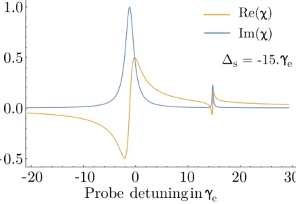
If we excite the atoms off-resonantly on the probe transition, then interesting fea-tures are observed near the two photon resonance [67,68]. The resonant absorption line remains almost unaffected while a second absorption/dispersion response is observed at ∆𝑒 ≈ −∆𝑐. This corresponds to a two-photon resonance, where the

atomic population is transfered from ground state to the meta stable one.

-20

-10

0

10

20

30

-0.5

0.0

0.5

1.0

Probe detuningin 

Im()

Re()

∆

= -15.



Figure 2.9: Two-photon resonance response: The real and the imaginary part of the susceptibilities of a system when the control field is detuned by -15𝛾𝑒, its

Rabi frequency is set to 5𝛾𝑒 and the linewidth is taken as 0.1𝛾𝑒. This creates a

sharp medium response at two photon resonance.

2.4.3 Multilevel system

In degenerate energy systems like Rydberg D states where multiple magnetic sub-levels are degenerate any weak electric fields can lead presence of more than three levels in the system refer Sec:7.5.2. Here we calculate how the transmission of the system is modified in the presence of more than one metastable state. We assume

that we are in a linear excitation regime (where ⟨𝜎(𝑖)

𝑔𝑔⟩ ≫ ⟨𝜎(𝑖)𝑒𝑒⟩). The extra

Hamil-tonian terms are ˆ ℋ𝑒𝑥𝑡= Ω𝑠′ 2 ∑︁ 𝑛 (ˆ𝜎_𝑠(𝑛)′_𝑒 + ˆ𝜎 (𝑛) 𝑒𝑠′) + Ω𝑠′′ 2 ∑︁ 𝑛 (ˆ𝜎_𝑠(𝑛)′′_𝑒+ ˆ𝜎 (𝑛) 𝑒𝑠′′)... (2.31)

We can define a new intermediate detuning term which can be written as ˜𝐷𝑒 =

𝐷𝑒− Ω 2 𝑠 4𝛿 − Ω2 𝑠′ 4𝛿 − Ω2 𝑠′′

4𝛿 . By evaluating the above expression we can evaluate the EIT

spectrum for multilevel atoms.

2.5 Non-linearity

The presence of a third level modifies the optical response in a non-trivial way. The two photon resonance in off-resonant excitation scheme exhibits a narrow response. This allows us to easily saturate the medium which gives rise to a non-linear optical response. Large non-linearities have been observed experimentally based on these schemes [63,68,69].

If we look at the expression for susceptibility, we can observe that the intracavity intensity is rescaled by the factor 1+ Ω2

𝑠

8𝛿2. One can observe large non-linearities with

even weaker probe fields by having a strong control field Rabi frequency. However, the effects cannot be described as “true” non-linearities because they are manifested from saturation of |𝑠⟩. The photons are just converted into atomic excitations in the other ground state. Even though compared to two level systems the number of photons required to observe the non-linearity has decreased, the number of atomic excitations are still of the same order. So, in order to observe strong non-linear effects we need an extra feature which doesn’t convert the photons into atomic excitations. As we will see in the next chapter, atoms excited to |𝑠⟩ must exhibit long range interactions, which will render the remaining atoms further detuned from the optical fields.

Chapter

3

Rydberg-Rydberg Interactions

Contents

3.1 Introduction . . . 25

3.2 Mean field approach . . . 27

3.3 Rydberg bubble model . . . 28

3.1 Introduction

As we have shown in the previous chapter that non-linearities obtained using multi-level or EIT schemes are not strong enough to be observed at single photon multi-level. To achieve this we need some kind of interaction between the atoms which can modify the behavior of the cloud even with few polaritons in the system. The promising solution is to use highly excited Rydberg atoms. The remarkably properties exhib-ited by atoms excexhib-ited to Rydberg states will help us in realizing strong interatomic interactions [70].

Atoms excited to a very high principal quantum number, higher than 30 are referred as Rydberg atoms. They have long lifetimes (few 100 𝜇s) and large dipole moments, which makes them sensitive to weak perturbations in their environments [71]. This large dipole moment creates a dipole potential through which it can interact with neighbouring atoms over long distances (few microns). Rydberg-Rydberg interactions have several degrees of freedom, one can control the type of interactions, the distance and the direction by selecting a Rydberg state. By mapping photons onto Rydberg excitations one can achieve exotic states of photons or strong non-linear interactions.

The dipole-dipole interaction energy between neutral dipoles separated by a distance ‘R’ is given by 𝑉𝑑1,𝑑2(𝑅) = 1 4𝜋𝜀0 [︂ 𝑑1.𝑑2 |𝑅|3 − 3 (𝑑1.𝑅).(𝑑2.𝑅) |𝑅|5 ]︂ (3.1) In order to evaluate the interacting two-atom system, one needs to take into account mainly the neighboring Rydberg energy levels which contribute the

signifi-r ~ n2_a 0 -5 -4 -3 -2 -1 0 5S_1/2 5D_5/2 5P_1/2 5P_3/2 E (eV) L = 0 L = 1 L = 2

Figure 3.1: Quantized energy levels of Hydrogen-like atoms: The electronic energy levels for low angular momentum states are plotted. The valence electrons for low angular momentum states spend more time closer to the nucleus, hence need more energy to ionize. In the inset: The Rydberg atomic radius increases with the square of principal quantum number (n2_{). The valence electron can move up to}

few microns away from the nucleus for n = 140.

cantly to the interaction. If we consider two atoms with atomic states |𝑟1⟩, |𝑟2⟩and

|𝑟3⟩. We assume that the pair states |𝑟2𝑟2⟩ and |𝑟1𝑟3⟩ are separated by ∆ and the

state |𝑟2𝑟2⟩ is coupled to |𝑟1𝑟3⟩ by 𝑉 (𝑅). The eigenenergies of pair system can be

written as

𝐸± =

∆ ±√︀∆2_{+ 4𝑉 (𝑅)}2

2

The eigenenergies of the total Hamiltonian can be described in two different regimes: the Van der Waals regime, and the dipole-dipole regime. One in which the interaction term is much smaller than the energy difference (𝑉 (𝑅) ≪ ∆) it is referred to as off-resonant Van der Waals interactions, and at the other extreme where the interaction term is much larger than the detuning (𝑉 (𝑅) ≫ ∆) are called as resonant dipole-dipole interactions.

In the Van der Waals regime the eigenenergies are shifted by (∆𝐸 ∝ 𝐶6/𝑅6)

and in the resonant dipole-dipole regime they are shifted by (∆𝐸 ∝ 𝐶3/𝑅3). This

dipole interaction strength 𝐶3 and 𝐶6 scales as (𝑛*)4 and (𝑛*)11 respectively.

These interactions lead to a Rydberg level detuned out of resonance and the con-trol field is no longer resonant with the secondary transition, this effect is known as Rydberg blockade effect. The medium then acts as two-level atoms and the absorption dominates. They are currently one of the most actively researched can-didates in quantum optics for generating non-classical states or quantum effects using dipole-dipole interactions [72].

The Rydberg-Rydberg interaction Hamiltonian term between atoms in Rydberg state |𝑟⟩ is [47] ℋ𝑖𝑛𝑡= 1 2 ∑︁ 𝑚̸=𝑛 𝜅𝑚,𝑛𝜎ˆ𝑟𝑟(𝑚)𝜎ˆ (𝑛) 𝑟𝑟 (3.2)

3.2. Mean field approach

(a)

(b)

|g,g〉

|r,g〉,|g,r〉

|r,r〉

V

(r)

Figure 3.2: Rydberg-Rydberg Interactions: (a) Two interacting Rydberg atoms separated by a distance r. (b) The energy levels of the combined two atom system. If the excitation linewidth is lower than the V𝑖𝑛𝑡(𝑟) then it is not possible to reach

the |𝑟, 𝑟⟩ state.

The Bloch equations for the coherence terms can be derived from the total Hamil-tonian along with the interaction term, leading to the following equations.

𝑑 𝑑𝑡𝜎ˆ (𝑛) 𝑔𝑒 = 𝑖(∆𝑒+ 𝑖𝛾𝑒)ˆ𝜎𝑔𝑒(𝑛)+ 𝑖𝑔ˆ𝑎(ˆ𝜎 (𝑛) 𝑒𝑒 − ˆ𝜎 (𝑛) 𝑔𝑔 ) − 𝑖 Ω𝑐𝑓 2 𝜎ˆ (𝑛) 𝑒𝑟 + ˆ𝐹 (𝑛) 𝑔𝑒 𝑑 𝑑𝑡𝜎ˆ (𝑛) 𝑒𝑟 = 𝑖(𝛿 + 𝑖𝛾𝑒𝑟)ˆ𝜎𝑒𝑟(𝑛)+ 𝑖𝑔𝑎 † ˆ 𝜎(𝑛)_𝑔𝑟 + 𝑖Ω𝑐𝑓 2 (ˆ𝜎 (𝑛) 𝑟𝑟 − ˆ𝜎 (𝑛) 𝑒𝑒 ) − 𝑖ˆ𝜎 (𝑛) 𝑒𝑟 ∑︁ 𝑚̸=𝑛 𝜅𝑚,𝑛𝜎ˆ(𝑚)𝑟𝑟 + ˆ𝐹 (𝑛) 𝑒𝑟 𝑑 𝑑𝑡𝜎ˆ (𝑛) 𝑔𝑟 = 𝑖(∆𝑟+ 𝑖𝛾𝑟)ˆ𝜎(𝑛)𝑔𝑟 + 𝑖𝑔ˆ𝑎ˆ𝜎 (𝑛) 𝑒𝑟 − 𝑖 Ω𝑐𝑓 2 𝜎ˆ (𝑛) 𝑔𝑒 − 𝑖ˆ𝜎 (𝑛) 𝑔𝑟 ∑︁ 𝑚̸=𝑛 𝜅𝑚,𝑛𝜎ˆ𝑟𝑟(𝑚)+ ˆ𝐹 (𝑛) 𝑔𝑟 (3.3) where 𝐹(𝑛)

𝑖𝑗 is the Langevin noise operator corresponding to the operator ˆ𝜎 (𝑛) 𝑖𝑗 , 𝛿 =

∆𝑒+ ∆𝑠 is two photon detuning term and Ω𝑐𝑓 is the control field Rabi frequency

(|𝑒⟩ → |𝑟⟩). The interaction term is restricted to the symmetric subspace, where states are invariant under the permutation of two particles and 𝜅𝑚,𝑛 is interaction

energy between atoms m and n in Rydberg state. This interaction term is a function of 𝐶6 in the case of Van der Waals interaction and 𝐶3 for resonant dipole-dipole

interaction.

The interaction term in the Hamiltonian is an N body problem and it cannot be solved without making some approximations like the mean field approach. Here we will describe two such methods which we use to explain our Rydberg non-linearity measurements. The models have been developed by Andrey Grankin and Etienne Brion, they are well described in A. Grankin’s thesis [73].

3.2 Mean field approach

The computation of the non-linear response of N body interactions scales exponen-tially and becomes intractable for even few atoms. One way to circumvent this problem is by using a mean field approach [74,75] where each atom’s response is modified by a mean field it experiences from its neighboring atoms.

We introduce two new collective atomic operators corresponding to the transi-27