Meteorology and air-quality in a mega-city: application to Tehran, Iran

(1)

HAL Id: pastel-00555962

https://pastel.archives-ouvertes.fr/pastel-00555962

Submitted on 14 Jan 2011

HAL is a multi-disciplinary open access archive for the deposit and dissemination of sci-entific research documents, whether they are pub-lished or not. The documents may come from teaching and research institutions in France or abroad, or from public or private research centers.

L’archive ouverte pluridisciplinaire HAL, est destinée au dépôt et à la diffusion de documents scientifiques de niveau recherche, publiés ou non, émanant des établissements d’enseignement et de recherche français ou étrangers, des laboratoires publics ou privés.

Hossein Malakooti

To cite this version:

Hossein Malakooti. Meteorology and air-quality in a mega-city: application to Tehran, Iran. Meteo-rology. Ecole des Ponts ParisTech, 2010. English. �NNT : 2010ENPC1001�. �pastel-00555962�

(2)

PhD thesis of École des Ponts ParisTech

Presented and publicly defended on January 21, 2010 by

Hossein MALAKOOTI

for obtaining the PhD degree of École des Ponts ParisTech / Universite Paris Est

Specialty: Science and technology environment

Meteorology and air-quality in a mega-city:

application to Tehran, Iran

The defense committee was consisted of

Matthias BEEKMANN LISA laboratory, CNRS & University Paris XII and VII

President

Alain CLAPPIER LIVE laboratory, University of Strasbourg Reviewer Abbas-Ali ALI-AKBARI BIDOKHTI Institute of Geophysics, University of Tehran Reviewer

Bruno SPORTISSE INRIA Thesis Supervisor

Sylvain DUPONT EPHYSE research unit, INRA Referee

Maya MILLIEZ EDF Research & Development Referee

(3)

(4)

)

i

(

was examined in the complex-terrain, semi-arid Tehran region using the Pennsylvania State University/National Center for Atmospheric Research fifth-generation Mesoscale Model (MM5) during a high pollution period. In addition, model sensitivity studies were conducted to evaluate the performance of the urban canopy and urban soil model "SM2-U (3D)" parameterization on the meteorological fields and ground level air pollutant concentrations in this area. The topographic flows and urban effects were found to play important roles in modulating the wind and temperature fields, and the urbanized areas exerted important local effects on the boundary layer meteorology. An emission inventory of air pollutants and an inventory of heat generation were developed and updated for 2005 in this work. Emissions from on-road motor vehicles constitute a major portion of the emission inventory and play the most important role in terms of contributions of air pollutants to the atmosphere in Tehran. By using a detailed methodology, we calculated spatial and temporal distributions of the anthropogenic heat flux (Qf) for Tehran during 2005. Wintertime Qf is larger than summertime Qf, which reflects the importance of heating emissions from buildings and traffic during cold and warm period respectively.

Different urban parameterizations were used as a tool to investigate the modifications induced by the presence of an urban area in the area of interest. It was found that, for local meteorological simulations, the drag-force approach coupled with an urban soil model (DA-SM2-U) is preferable to the roughness approach (RA-SLAB). The comparisons indicated that the most important features of the wind, temperature and turbulent fields in urban areas are well reproduced by the DA-SM2-U configuration with the anthropogenic heat flux being taken into account (i.e., "DA-SM2-U Qf: On" option). This modeling option showed that the suburban part of the city is dominated by topographic flows whereas the center and south of Tehran are more affected by urban heat island (UHI) forcing especially during the night.

The chemical transport modeling, including a model sensitivity study, was used to investigate the impact of the different urban parameterization on the dispersion and formation of pollutants over the Tehran region. Results show that applying DA approaches leads to significant improvements in the simulated spatial and temporal distribution of air pollutant concentrations in the city area and affects significantly the size of the urban plumes.

(5)

)

ii

(

of his guidance and for correction of the manuscript. I wish to acknowledge the Islamic Republic of Iran Meteorological Organization (IRIMO), Tehran air pollution control company (AQCC), Institute of Geophysics (University of Tehran), Iran Department of environment (DOE), Tehran Gas Company (TGC), Tehran Province Regional Electricity Company (TREC)’s Consumption Management Administration for providing essential data. Funding was provided by CEREA, Joint Laboratory École des Ponts ParisTech (Université Paris-Est) /EDF R&D and Hormozgan University (Bandar Abbas, Iran).

(6)

) iii (

The atmospheric boundary layer (ABL), also known as the planetary boundary layer (PBL) is the lowest portion of the troposphere. Stull (1988) defines PBL as “that part of the atmosphere that is directly influenced by the presence of the Earth’s surface, and responds to surface forcings with a time scale of about an hour or less”.

The majority of the global population currently lives and works in urban areas, and this urbanization is expected to increase. According to the United Nations, population projections (UN, 2006) suggest that the global proportion of urban population will increase from 49 % in 2005 to 60 % in 2030.

The urban surface morphology (presence of buildings), urban materials, vegetation differences and human activities profoundly modify the PBL structure over urban areas. This has important implications for the transport and dispersion of pollutants (most of anthropogenic effluents that are emitted from sources within the PBL), photochemical processes, urban design, energy usage studies, thermal comfort level evaluations, etc. It is reported that in most of mega-cities, air pollution is worsening because of increased industry, vehicles and population. Managing waste, treating sewage, reducing noise, reducing pollutant emissions to control air quality have become challenges for planners and decision makers at all levels. The processes leading to urban air pollution are diverse, interrelated, complex and non-linear. Extended knowledge on the type, quantity, residence time and sources of the pollutants emitted in the urban atmosphere is necessary,

(10)

in order to reduce the human health effects in an effective manner. Special urban network of air quality and meteorology measurements and extensive emissions studies are conducted in order to give an overview of the cities situations. Associating these data to modeling tools makes it possible to provide decision-support and forecast tools to planners and governments to design pollutant emissions abatement strategies. Understanding and forecasting air quality in urban areas has emerged as an active field of research with clear socio-economics demands.

Tehran, the Capital of Iran, is faced with many socio-economic and environmental problems. The environmental problem that affects people more than any other in Tehran is air pollution.

Tehran’s air quality has been deteriorated over time due to the cumulative effects of rapid population growth, a large and old vehicle fleet (mobile sources), a large number of industrial and commercial establishments (stationary sources), its geographical location , including an ensnared condition as it is surrounded by ranges of mountains, and also the lack of perennial winds. Urban transport is the leading cause of this problem. More than one decade ago, the Government of the Islamic Republic of Iran identified Tehran’s air pollution problem as a high priority environmental and health issue (Global Environment Facility, 1993).

1.1 Scale and the urban surface

Meteorological phenomena can be classified as functions of their temporal and spatial scales. Urban meteorology covers phenomena with four typical ranges of spatial scales. For example, Britter (2003) used the following spatial scales to describe the major urban flow features: regional scale (up to 100 or 200 km), city scale (up to 10 or 20 km), neighborhood scale (up to 1 or 2 km), and street scale (less than 100 to 200 m). The complex urban morphology lead to various physical-chemical processes which have effects at different scales (meso-micro) and hence, a mega-cities can play quite a significant role on regional weather.

Consequently, numerical air quality models, which constitute a robust approach to manage and forecast air pollution, require an integrated approach to simulate both the

(11)

local urban scale and the mesoscale city surroundings. Here are two modeling approaches at respectively local and mesoscale:

I) The street canyon models provide spatially detailed results, but they are restricted to small areas (one to a few streets) and generally decoupled from the larger scale circulation (which limits their accuracy to short time intervals and near source distance). They are adapted to study the air quality in the streets but cannot be used to simulate the development of the urban plume.

II) The mesoscale models cover a relatively large area (domains of the order of 100-200 km), but their spatial resolution (typically 1 to 10 km horizontally and a few tens of meters in the vertical) does not allow one to reproduce the detailed structure of the urban areas. Consequently, sub-grid surface fluxes and turbulence parameterizations are necessary in order to take into account the significant perturbations induced by the cities.

Since an integrated approach, both at the local and regional level, is necessary, a full coupling of the two approaches (insertion within each mesoscale grid cell of a street canyon model) seems to be an ideal approach. But it is computationally expensive proces. For this reason, the urban parameterization method, which consists of taking into account the effects of buildings and streets in a mesoscale model through turbulence parameterizations, represents a better compromise.

In order to develop urban canopy parameterizations, we need descriptions and classifications of urban landuse geometry. The methods that are typically used to introduce urban modifications inside meso-scale meteorological models (MMMs) are mostly based on averaging out the variations in parameters around individual buildings. The general parameters used to classify the urban surface morphology include building height he, the plane area density λP, and the frontal area density λF (e.g., Grimmond and Oke, 1999b) averaged over the scale of interest. Similar information on vegetation canopies is also used. These morphological parameters are illustrated in Figure 1.1.a for an array of uniform buildings. They are defined as follows: λ_P = A_P /A_T = L_xL_y /D_xD_y

and λ_F = A_F /A_T = z_HL_y /D_xD_y. One other method consists of using two parallel buildings, that are uniform in height and size with flat roofs as shown in Figure 1.1.b

(12)

(under the flow normal to the canyon axis). In this method, key morphological parameters are defined as follows:

λ

_f

=

h /

_e

r

_e and

λ

_p =1−

ω

_e /r_e.

a) b)

Figure 1.1: Schematic representation of the non-dimensional morphometric ratios for an

array of uniform buildings (after Grimmond and Oke, 1999b).

In order to better represent the urban canopy and its effects in MMMs, one method that is often considered consists of having several layers of the model within canopies. In this method λP and λF are estimated for each kind of canopies and surfaces, and are distributed according to the fraction in each model layer within the urban canopies (adapted from Brown and Williams 1998, Martilli 2002 and Dupont et al. 2004). This method is illustrated for urban buildings in Figure 1.2.

Figure 1.2: Schematic illustration of side view of an urban canopy representation. The area of

interest is partitioned into areas defined as urban and nonurban. The canyon regions are defined in the areas between buildings, and the sum of the canyon areas is f cnyn. The remainder of f urb is defined as f roof. There are several model layers (shown as dashed lines) within the urban canopy layer.

(13)

1.2 The urban boundary layer

The bottom of the boundary layer is modified by the urban surface features and the depth of this modified layer increases with distance downwind from these structure or vegetation. This modified layer is called the internal boundary layer (IBL). Above it, the air flow continues behaving as it did upwind of the structures (Stull, 1998). The internal boundary layer is influenced by, but not fully adjusted to, the structures of the new surface and it deepens with fetch.

The internal boundary layer formed over urban areas is called the urban boundary layer (UBL). When a new rural boundary layer forms at the surface downwind of the urban area, the urban boundary layer is isolated aloft and is then called the urban plume. The flow in the urban canopy layer (beneath the mean height of the buildings and trees) is highly heterogeneous spatially and subjected to a drag force (Belcher et al., 2003). The Urban Canopy Layer (UCL) is a zone of multiple effects on the PBL structure. We classify these effects into four categories: dynamic, thermodynamic, anthropogenic heating and air pollution effects. Table 1.1 summarizes the general micrometeorological effects of urban canopies. These effects alter temperature and wind fields over the urban environment and contribute to the formation of the Urban Heat Island (UHI). The UHI is typically presented as a temperature difference between the air within the UCL and that measured in a rural area outside the settlement (Mills, 2004).

UBL and urban plume are presented in Figure 1.3. The UBL is, however, a collection of successive IBLs rather than one single internal boundary layer, because of continual evolution of dynamic - thermodynamic processes across the urban area.

The UBL has a vertical structure more complex than that of the boundary layer in rural areas and it is normally partitioned into a canopy layer, a roughness sub-layer (RSL), an inertial sub-layer (ISL) and a mixed layer, depending on the characteristics of the mean and turbulent parts of the flow (e.g. Garratt, 1992).

(14)

Figure 1.3: a) Schematic structure and potential temperature profiles (θ) by day (top) and at

night (down) of the UBL in a large city during fine weather (after Oke, 1982) and b) Schematic of the boundary layer over an urban surface with typical depths for the sub-layers (e.g. Roth, 2000). zi is the depth of the planetary boundary layer over an urban area.

Table 1.1 The general micrometeorological effects of urban canopies.

UCL features Effects

Urban canopy geometry Different spatial distribution of turbulence and wind

Increased net-shortwave radiation (increased surface area and multiple reflection)

Decreased net-longwave radiations (reduced sky view factor) Decreased and latent heat fluxes (reduced wind speed)

Construction materials Increased heat storage (increased thermal admittance) Decreased latent heat flux (increased water-proofing) Increased net-shortwave radiation (reduced surface albedo)

Anthropogenic heating Effect of heat production from fuel and electricity consumption in building and transportation sectors as well as metabolism

Air pollution Increased sky longwave radiation (Greater absorption and re-emission)

There are several key differences in the nature of the turbulence over rural and urban sites, such as significant dispersive stresses within urban canopies (Cheng and Castro, 2002), Reynolds stress peak at or just above roof level (e.g., Rotach, 1993a), leading to an alteration of turbulent spectrum over urban areas. The peak in the energy spectrum is flattened with no single frequency dominating the power spectrum (Louka, 1998; Roth, 2000). In the RSL, in fact, the flow is influenced more by the local geometry than by a

(15)

homogeneous energy transfer between horizontal layers. The flow regimes in urban street canyons can be categorized into the isolated roughness flow, the wake interference flow, and the skimming flow, depending on the canyon aspect ratio (he/we) and uniformity of the building height. These flow regimes are determined by the degree of interaction between the vortex generated behind the upwind building and the downwind building (Hussain and Lee 1980; Oke 1988; Hunter et al. 1992; Sini et al. 1996). Three flow regimes may form depending on the ratio (he/we). The inherent features of the three flow regimes are schematically drawn in Figure 1.4.

The RSL extends from the surface up to a height at which the influence of individual roughness elements on the flow is 'mixed up' by turbulence (Raupach et al., 1991), and the flow can be considered horizontally homogeneous if the density, height and distribution of roughness elements do not vary over the upwind area of influence. The depth of RSL is estimated to be 1.8–5 building heights and it has been shown to depend on the stability, separation of the buildings and building shape (Raupach et al., 1980; Oke, 1987; Rafailidis, 1997; Roth, 1999; Roth, 2000; Cheng and Castro, 2002).

Figure 1.4: Flow regimes in UCs: (a) isolated roughness flow (he/we ≤0.3), (b) wake interference flow (he/we intermediate), and (c) skimming flow (he/we≥0.7) from Oke (1987).

(16)

The classical techniques used to represent surface effects in mesoscale models are based on the Monin-Obukhov Similarity Theory (MOST) and aerodynamic characteristics of the urban surface are often represented using various approaches:

I) The roughness approaches (RA) uses an area-specific roughness length and a displacement height (Roughness approach: RA) (e.g. Venkatram, 1980; Bottema, 1997), which assumes stationary conditions and spatial homogeneity.

II) The empirical models are based on observations of the urban surface energy balance (Grimmond et al., 1998; Grimond and Oke, 1999a). These models use extremely simple schemes, but they need many measurements data and are limited to the range of those data conditions (city, land cover, climate, season, etc).

III) The schemes adapted from plant canopies are the most common way to simulate the urban surface energy balance. This approach is based on the adaptation of the thermal and mechanical properties of a rural area in a soil vegetation transfer scheme (Todhunter and Werner, 1988 ; Dupont et al., 2002).

IV) For radiative effects and the energy balance, surface albedo is generally decreased, the ground is "dried", the soil heat capacity is modified and anthropogenic fluxes are sometimes prescribed as additional energy source (Makar et al., 2006).

These approaches are not able to take into account the geometry of the buildings and do not reproduce the radiative transfers between the different urban surfaces.

Furthermore, the MOST profiles are not valid below the displacement height (the lowest model level at which RA applies) and RA does not reproduce the turbulent kinetic energy (TKE) maximum observed just above the urban canopy. Also field measurements (e.g., Rotach, 1993b) have shown that RA is not able to reproduce the vertical structure of the turbulent fields in urban RSL.

Recently, in order to better represent realistic 3D urban canopy effects (urban canopy parameterization: UCP), the drag force approach has been applied to account for the drag induced by the buildings, as well as comprehensive canopy surfaces (wall, roof, road) energy balance inside MMMs. This UCP can be either single layer (Masson, 2000) or a multi-layer buildings parameterization (Vu et al., 1999; Martilli et al., 2002; Kondo et al., 2005). The single-layer parameterization concerns only the first level of MMMs, whereas

(17)

the multi-layer parameterization can impact all levels directly influenced by the buildings. In this study we use a multi-layer UCP developed by Martilli et al. (2002) and Dupont et al. (2004).

The flow and potential temperature in the inertial sub-layer are horizontally homogeneous and MOST may be applicable in this sub-layer. The mixed layer is normally covered by an inversion layer at the top of UBL and during the day, flow and potential temperature are rapidly mixed resulting in horizontally homogeneous, vertically uniform profiles in the mixed layer, during the night this sub-layer may be further partitioned into a residual mixed layer of the previous day overlying a stable surface layer which has been cooled from below (Roth, 2000).

1.3 Urban canopy parameterization in MMMs

Brown (2000) has reviewed some methods in order to improve the representation of urban RSL characteristics in mesoscale models. The improvement of the urban canopy representation in mesoscale models requires knowledge of various parameters that can be divided into three categories:

I) The empirical parameters, which are deduced from calibration of the models,

II) The “material parameters”, which correspond to the physical properties of the surface materials of the canopy elements,

III) The morphological parameters, which depend on the structure and on the 3D arrangement of the canopy elements (buildings, vegetation, etc).

The morphological parameters are variable from one city to another and need to be averaged over a few 100 m2 with a vertical resolution of a few meters to be used at neighborhood scales. Thus, these parameters may be the most difficult parameters to estimate.

The recent UCPs based on the drag-force approach take into account the dynamic, thermodynamic and turbulent effects of urban canopies by adding terms in the conservation equations:

(18)

I) in the dynamic equation, a friction force induced by horizontal surfaces of buildings, and a pressure and viscous drag force induced by the presence of buildings and vegetation;

II) in the temperature equation, the sensible and latent heat fluxes from buildings and vegetation and the anthropogenic heat flux parameterized following Taha (1999); III) in the specific humidity equation, the humidity sources coming from the

evapotranspiration of the vegetation and the evaporation of the water intercepted by buildings;

IV) in the turbulent kinetic energy equation, a shear and buoyant production terms induced by buildings and vegetation, turbulent kinetic energy sources induced by the presence of buildings and vegetation.

Furthermore, soil and water budget models are developed for urban area because of multi cover fractions such as bare, paved, vegetated and mixed (i.e., combination of those) surfaces, lakes, irrigation areas, etc. Those models are important to improve the evaporation, since the urban latent heat flux may have a large influence on micro scale phenomena.

In these models, the lower level of the computational domain corresponds to the real level of the ground. The volume of buildings is considered in each cell and additional vertical layers are included within the canopy to allow more detailed meteorological fields within the RSL.

(19)

1.4 Urban air quality

High levels of pollution adversely affect most of the populated regions. Air pollution is one of several important environmental hazards alongside with water contamination, hazardous waste, noise and others. It is currently an important environmental concern of large cities.

Swelling urban populations and increased concentration of industry and automobile traffic in and around cities have resulted in severe air pollution. Emissions from traffic, factories, domestic heating, cooking and refuse burning are threatening the health of city dwellers, imposing not just a direct economic cost by impacting human health but also threatening long-term productivity.

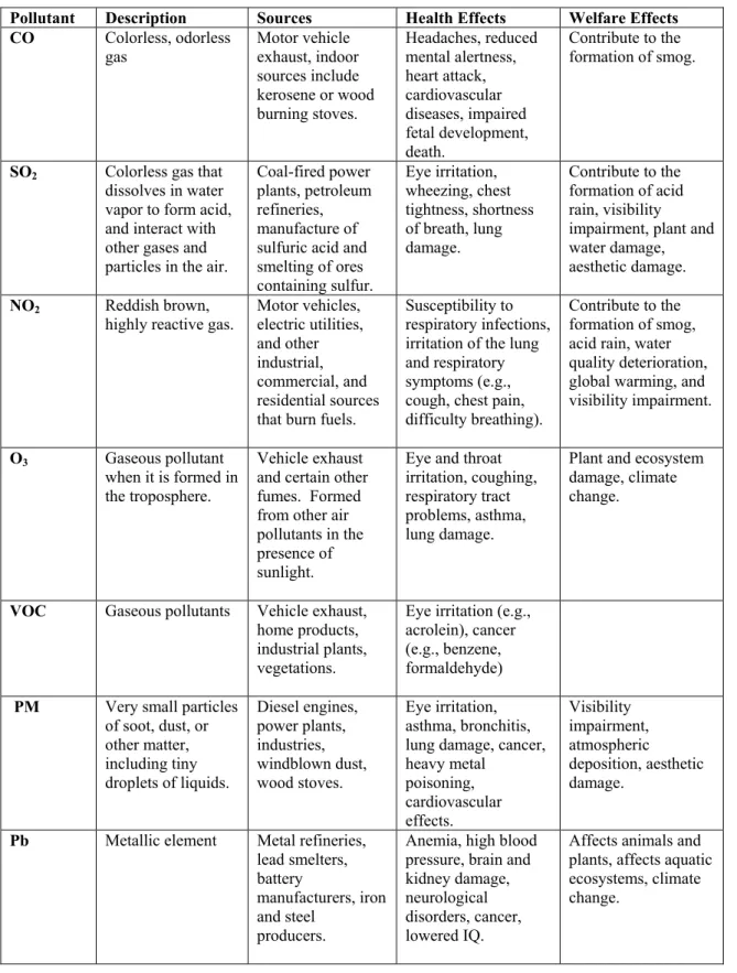
Basic urban pollutants (Fenger, 1999) include sulphur dioxide (SO2), nitrogen oxides (NOx), carbon monoxide (CO), volatile organic compounds (VOC), ozone (O3), particulate matter (PM) and lead (Pb).

Exposure to air pollution is associated with numerous effects on human health, including pulmonary, cardiac, vascular and neurological impairments. High-risk groups such as the elderly, infants, pregnant women and sufferers from chronic heart and lung diseases are more sensitive to air pollution than the general population. Exposure to air pollution can cause both acute (short-term) and chronic (long-term) health effects. Acute effects are usually immediate and often reversible when exposure to the pollutant ends. Some acute health effects include eye irritation, headaches and nausea. Chronic effects are usually not immediate and can be irreversible. Some chronic health effects include decreased lung capacity and lung cancer. Table 1.2 summarizes the sources, health and welfare effects for selected pollutants. Hazardous air pollutants may cause other less common but potentially hazardous health effects, including cancer, damage to the immune system, and neurological, reproductive and developmental problems. Acute exposure to some hazardous air pollutants can cause immediate death. Human health effects associated with indoor air pollution are: headaches, tiredness, dizziness, nausea, and throat irritation. More serious effects include cancer and exacerbation of chronic respiratory diseases, such as asthma. Asthma, particularly for children, can result from poor indoor air quality. Air

(20)

pollutants can also enter into our body by drinking and eating following deposition on to an ecosystem and subsequent bioaccumulation. There are many harmful welfare effects of air pollution: acid rain, climate change, depletion of stratospheric ozone, damage to agricultural crops, and decreased visibility.

Air pollutants are classified into two categories. Primary pollutants are directly emitted into the atmosphere, such as NOx and VOCs and secondary pollutants are formed in the atmosphere as a result of chemical transformation of the primary pollutants. Secondary pollutants include tropospheric ozone (O3) created in a reaction cycle involving NOx, CO and VOC and which occurs in the presence of solar energy.

Primary pollutants act in situ, i.e., mainly in the cities where traffic and industrial activities are the highest, while secondary pollutants often affect the environment (as in the case of ozone) in rural areas. For example, ozone formation occurs relatively close to the ground in the plume downwind of primary pollutant emission, usually at distances of 10 to 100 km from the sources, when VOC and NOx are both present in relevant quantities (see Figure 1.5).

This difference leads to a difficult situation for policy makers dealing with air quality management. The problems become even more complex for pollutants such as ozone and PM that are subject to transcontinental pollutant transport, which occur in the stratosphere.

(21)

Table 1.2: Sources, health and welfare effects for selected Pollutants (Ref: US EPA website). Pollutant Description Sources Health Effects Welfare Effects CO Colorless, odorless

gas Motor vehicle exhaust, indoor sources include kerosene or wood burning stoves. Headaches, reduced mental alertness, heart attack, cardiovascular diseases, impaired fetal development, death. Contribute to the formation of smog.

SO2 Colorless gas that

dissolves in water vapor to form acid, and interact with other gases and particles in the air.

Coal-fired power plants, petroleum refineries, manufacture of sulfuric acid and smelting of ores containing sulfur. Eye irritation, wheezing, chest tightness, shortness of breath, lung damage. Contribute to the formation of acid rain, visibility impairment, plant and water damage, aesthetic damage.

NO2 Reddish brown,

highly reactive gas. Motor vehicles, electric utilities, and other industrial, commercial, and residential sources that burn fuels.

Susceptibility to respiratory infections, irritation of the lung and respiratory symptoms (e.g., cough, chest pain, difficulty breathing).

Contribute to the formation of smog, acid rain, water quality deterioration, global warming, and visibility impairment.

O3 Gaseous pollutant

when it is formed in the troposphere.

Vehicle exhaust and certain other fumes. Formed from other air pollutants in the presence of sunlight.

Eye and throat irritation, coughing, respiratory tract problems, asthma, lung damage.

Plant and ecosystem damage, climate change.

VOC Gaseous pollutants Vehicle exhaust, home products, industrial plants, vegetations.

Eye irritation (e.g., acrolein), cancer (e.g., benzene, formaldehyde)

PM Very small particles of soot, dust, or other matter, including tiny droplets of liquids. Diesel engines, power plants, industries, windblown dust, wood stoves. Eye irritation, asthma, bronchitis, lung damage, cancer, heavy metal poisoning, cardiovascular effects. Visibility impairment, atmospheric deposition, aesthetic damage.

Pb Metallic element Metal refineries, lead smelters, battery

manufacturers, iron and steel

producers.

Anemia, high blood pressure, brain and kidney damage, neurological disorders, cancer, lowered IQ.

Affects animals and plants, affects aquatic ecosystems, climate change.

(22)

Figure 1.5: physical, chemical and environmental processes of urban plume.

The pollutants concentrations in the ambient outdoor air depend on emissions, background concentrations, chemical, transport–diffusion and deposition processes (Mayer, 1999). All these processes explicitly depend on meteorological parameters such as radiation, stability, wind, temperature, turbulence, rain, humidity, etc.

A combination of state-of-the-science measurements with state-of-the-science models is the best approach for making real progress toward understanding atmospheric processes. A model involving descriptions of emission patterns, meteorology, chemical transformations and removal processes is an essential tool for the appropriable approach. Such a model provides a link between emission changes from source control measurements and resulting changes in airborne concentrations (Seinfeld and Pandis, 1998; B. Sportisse, 2008).

Meteorological inputs constitute one of the main sources of uncertainty in chemistry transport models (CTMs), especially in urban areas, because of high influence of urbanization on local climates. Therefore, a correct treatment of meteorology is essential for accurate air quality modeling.

(23)

1.5 Overview of Tehran characteristics

With the location 35° 41' N - 51° 25' E and altitude of 1000-1800 meters above mean sea level, Tehran, capital of Iran, is located on the southern slope of the Alburz mountain chain. Its climate is generally moderate to dry. During the last 3 to 4 decades, urban expansion in Tehran resulted from a high rate of population growth and rural-urban migration combined with a strong tradition of centralization and dense urban infrastructure. As a result, there has been an over increasing trend in energy consumption in the capital. Tehran is located in valleys and is surrounded on the north, northwest, east and southeast by high to medium high (3800-1000 m) mountain ranges (see Figure 1.6). The northern part with more rainfall and vegetation is about 600-700 meter higher than the southernmost part which borders central deserts of Iran (Madanipour, 1999; Ketabi, 2004). The meteorological fields in Tehran are influenced by these geographical features. Because of these morphological conditions, generally weak winds and urban effects such as anthropogenic heating, Tehran experiences a significant UHI. Therefore, we believe that taking into account anthropogenic heating and other urban effects within a MM model sould improve the accuracy of meteorological simulations and better represent the local climate and circulations in this area.

The resident population of Tehran is about 8.3 millions according to the 2007 census (in contrast to two hundred thousands in 1920) and its daytime population is often more than 12 millions inhabitants on workdays, reflecting the highly dynamic spatial and temporal distribution of population in the greater Tehran urban area (670 km2). With a very large population, more than two million (often old) motor vehicles, fuel and electricity consumption and many factories (more than half of Iran’s industries are based in Tehran), huge quantities of pollutants and heat are emitted in this area.

Tehran is usually enveloped in a cloud of smog and, according to a recent study, each resident inhales between 7 and 9 kilograms of dust per year. The city has been rated as one of the most polluted cities on earth, suffering from increasing acute environmental problems such as air, water, land and noise pollution. Due to these facts air pollution is reported to significantly affect the quality of urban inhabitant’s life as well as to worsen urban environment and urban climate.

(24)

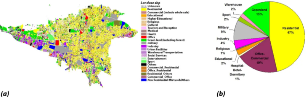
Figure 1.6: a) Geographical localization of Middle- East and Tehran, and b) landuse distribution (1: Urban,

2: Drylnd Crop. Past., 3: Irrg. Crop. Past. 4:Mix. Dry/Irrg.C.P., 5: Crop./Grs. Mosaic, 6: Crop./Wood Mosc, 7: Grassland, 8: Shrubland, 9: Mix Shrb./Grs., 10: Savanna, 11: Decids. Broadlf., 12: Decids. Needlf., 13: Evergrn. Braodlf., 14: Evergrn. Needlf., 15: Mixed Forest, 16: Water Bodies, 17: Herb. Wetland, 18: Wooded wetland, 19: Bar. Sparse Veg., 20: Herb. Tundra, 21: Wooden Tundra, 22: Mixed Tundra, 23: Bare Grnd. Tundra, 24: Snow or Ice and 0: No data) and c) topography of Tehran region.

(25)

The Pollutant Standards Index (PSI) system which was developed by the U.S.-EPA (e.g. National Air Quality and Emissions Trends Report, 1997) has been adopted by Tehran AQCC (Air Quality Control Company) for reporting daily air quality. The PSI provides a simple number on a scale of 0-500 related to the health effects of the air quality levels. Values of PSI during recent 18 years (after establishing a measurement network) show that air quality most often fell in the “moderate” category (50<PSI< 100) and had exceeded the threshold level (PSI = 100) in 75 to 169 days (20 - 46%) during one year. It is seen that carbon monoxide contributed 89% (8 hours average concentration more than 4.5 ppm) and PM 10 19% (24 hours average concentration more than 75 µgm-3_{) of critical} pollutants responsible for most of the unhealthy air quality days in Tehran. As shown in Figure 1.7, three months of August, September and October are the most polluted months in Tehran. 0 50 100 150 200 250 01/01/2002 01/01/2003 01/01/2004 01/01/2005 01/01/2006 01/01/2007 Dates PS I

Figure 1.7: PSI distribution during 2002-2006.

1.6 Thesis outline

This study has three main parts: emission improvement, local meteorology and chemistry transport modeling and their evaluations.

In the first part a high resolution mobile emission inventory is developed in order to prepare a Dynamic Emission Database (DEB) for this episode of the study. Traffic data are obtained from the EMME/2 transportation planning database and available observations by vehicle subcategories. The emission factors are adjusted with categories

(26)

and subcategories of Tehran vehicles, and along with this, the railway and aircraft emissions are also estimated. The evaluation of spatial distribution and diurnal variation of anthropogenic heat emission in Tehran region is also developed. The methods and estimated emissions are presented in Chapter 2.

In the second part, we study the boundary layer structure and its evolution, UHI influence and interaction between topographic and UHI flows in Tehran region. The urban canopy model introduced in MM5 by Dupont et al. (2004) is adapted, modified and tested for the Tehran basin. Thus, the roughness approach and Drag force approach are evaluated in this area. The methods and results are presented in Chapter 3.

The objective of the third part is a general study of modeling gases (CO, Ozone, NO2, etc.) and particular matters (PM10 and PM2.5). Simulations are evaluated and the sensitivity to meteorological inputs with different urban options is analyzed. This part is presented in chapter 4.

The results of this work and suggestions for future works in this area are summarized and discussed in Chapter 5.

(27)

References

Belcher, S.E., Jerram, N., and Hunt, J.C.R., 2003. Adjustment of a turbulent boundary layer to a canopy of roughness elements. Journal of Fluid Mechanics 488, 369-398.

Bottema, M., 1997. Urban roughness modeling in relation to pollutant dispersion. Atmospheric Environment 31, 3059-3075.

Britter, R. and Hanna, S. R., 2003. Flow and dispersion in urban areas. Annual Review of Fluid Mechanics 35, 469-496.

Brown, M.J. and Williams, M.D., 1998. An urban canopy parameterization for mesoscale models. Preprints, Second Urban Environment symposium, Albuquerque, New Mexico, American Meteor Society, 144-147.

Brown, M., 2000. Urban parameterizations for mesoscale meteorological models, in Boybeyi (ed.), Mesoscale Atmospheric Dispersion. Wessex Press, 448 pp.

Cheng, H. and Castro, I.P., 2002. Near wall flow over an urban-like roughness. Boundary Layer Meteorology 104, 229-259.

Dupont, S., Calmet, I., and Mestayer, P.G., 2002. Urban Canopy Modeling Influence on Urban Boundary Layer Simulation, in American Meteor Society 4th Symposium on Urban Environment, Norfolk, Virginia, 20-24 May , Proceedings, pp. 151-152. Dupont, S., Otte, T.L. and Ching, J.K.S., 2004. Simulation of meteorological fields within

and above urban and rural canopies with a mesoscale model (MM5). Boundary Layer Meteorology 113, 111-158.

Environmental Protection Agency, 1998. National Air Quality and Emissions Trends Report, 1997. Washington, DC: Author.

Fenger, J., 1999. Urban air quality. Atmospheric Environment 33, 4877-4900.

Garratt, J.R., 1992. The Atmospheric Boundary Layer. chapter 8, pages 224-257. Cambridge University Press.

Global Environment Facility, 1993. Tehran Transport Emissions Reduction Project. World Bank, Washington, DC.

(28)

Grimmond, C.S.B, King, T.S., Roth, M., Oke, T.R., 1998. Aerodynamic roughness of urban areas derived from wind observations. Boundary Layer Meteorology 89, 1-24.

Grimmond, C.S.B., Oke, T.R., 1999a. Heat storage in urban areas: local-scale observations and evaluation of a simple model. Journal of Applied Meteorology 38, 922-940.

Grimmond, C.S.B. and Oke, T.R., 1999b. Aerodynamic properties of urban areas derived from analysis of surface form. Journal of Applied Meteorology 38, 1262–1292. Harman, I.N., 2005. The energy balance of urban areas, Ph.D. thesis, Department of

Meteorology, University of Reading.

Hunter, L.J., Johnson, G.T., and Watson, I.D., 1992. An investigation of three-dimensional characteristics of flow regimes within the urban canyon. Atmospheric Environment 26B, 425-432.

Hussain, M., Lee, B.E., 1980. A wind tunnel study of the mean pressure forces acting on large groups of low-rise buildings. Journal of Wind Engineering and Industrial Aerodynamics 6, 207-225.

Ketabi, M., 2004. Sustainable Development in Tehran, A Case Study of Traffic and Pollution Problems in Tajrish District. Annual Meeting of the world student community for sustainable development (WSC-SD), Goteborg, Sweden.

Kondo, H., Genchi, Y., Kikegawa, Y., Ohashi, Y., Yoshikado, H., Komiyama, H., 2005. Development of a Multi-Layer Urban Canopy Model for the Analysis of Energy Consumption in a Big City: Structure of the Urban Canopy Model and its Basic Performance. Boundary Layer Meteorology 116, 395-421.

Louka, P., Belker, S.E., Harrison, R.G., 1998. Modified street canyon flow. Journal of Wind Engineering & Industrial Aerodynamics 74–76, 485-493.

Mayer, H., 1999. Air pollution in cities. Atmospheric Environment 33, 4029-4037. Madanipour, A., 1999. City profile: Tehran. Cities 16, 57-65.

Makar, P.A., Gravel, S., Chirkov, V., Strawbridge, K.B., Froude, F., Arnold, J., Brook, J., 2006. Heat flux, urban properties, and regional weather. Atmospheric Environment 40, 2750-2766.

(29)

Martilli, A., 2002. Numerical Study of Urban Impact on Boundary Layer Structure: Sensitivity to Wind Speed, Urban Morphology, and Rural Soil Moisture. Journal of Applied Meteorology 41, 1247-1266.

Martilli, A., Clappier, A., Rotach, M.W., 2002. An urban surfaces exchange parameterization for mesoscale models. Boundary Layer Meteorology 104, 261-304.

Masson, V., 2000. A physically-based scheme for the urban energy budget in atmospheric models. Boundary Layer Meteorology 94, 357-397

Mills, G., 2004. The Urban Canopy Layer Heat Island, IAUC Teaching Resources.

Oke, T.R., 1982. The energetic basis of the urban heat island. Quarterly Journal of the Royal Meteorological Society 108, 1-24.

Oke TR., 1987. Boundary Layer Climates. London, UK: Routledge ,435 p.

Oke, T., 1988. Street design and urban canopy layer climate. Energy and Buildings 11. pp. 103-113.

Rafailidis, S., 1997. Influence of building area density and roof shape on the wind characteristics above a town. Boundary Layer Meteorology 85, 255–271.

Raupach, M.R., Thom, A.S., and Edwards, I., 1980. A wind-tunnel study of turbulent flow close to regularly arrayed rough surfaces. Boundary-Layer Meteorology 18, 373–397.

Raupach, M.R., Antonia, R.A., Rajagopalan, S., 1991. Roughwall turbulent boundary layers. Applied Mechanics Reviews, 44, 1-25.

Rotach, M.W., 1993a. Turbulence close to a rough urban surface Part I: Reynolds stress. Boundary Layer Meteorology 65, 1-28.

Rotach, M.W., 1993b. Turbulence close to a rough urban surface Part II: variances and gradients. Boundary Layer Meteorology 66, 75-92.

Roth, M., 1999. On the influence of the urban roughness sub-layer on turbulence and dispersion. Atmospheric Environment 33, 4001-4008.

Roth, M., 2000. Review of atmospheric turbulence over cities. Quarterly Journal of the Royal Meteorological Society 126, 941–990.

(30)

Seinfeld, J.H., Pandis, S.N., 1998. Atmospheric Chemistry and Physics: From Air Pollution to Climate Change. Wiley, New York.

Sini, J.F., Anquetin, S., and Mestayer, P.G., 1996. Pollutant dispersion and thermal effects in urban street canyons. Atmospheric Environment 30, 2659–2677.

Sportisse, B., 2008. Pollution atmosphérique, Des processus à la modélisation. Springer, 345 p.

Stull, R.B., 1988. An Introduction to Boundary Layer Meteorology. Kluwer Academic Publishers. 666 p.

Taha, H., 1999. Modifying a mesoscale model to better incorporate urban heat storage: A bulk parameterization approach. Journal of Applied Meteorology 38, 466–473. Todhunter, P., Werner, T., 1988. Intercomparison of three urban climate models.

Boundary Layer Meteorology 42, 181-205.

United Nations: 2006, World Urbanization Prospects. The 2005 Revision, Department of Economic and Social Affairs, Population Division, New York.

Venkatram, A., 1980. Estimating the Monin-Obukhov length in the stable boundary layer for dispersion calculations. Boundary Layer Meteorology 19, 481.

Vu, T.C., Asaeda, T., Ashie, Y., 1999. Developpement of a numerical model for the evaluation of the urban thermal environment. Journal of Wind Engineering 81, 181-196.

(31)

-23-

Development and Evaluation of a High Resolution

Emission Inventory for Air Pollutants and

Heat Generation

2.1 Introduction

Urban agglomerations are major sources of regional and global atmospheric pollution as well as heat. This phenomenon is especially severe in cities of developing countries, where population, traffic, industrialization and energy use increase as people continue to migrate to the cities (Mage et al., 1996). Consequently, it is essential to develop energy and air quality management policies and to establish strategies for atmospheric pollution prevention and energy management for such cities. Main limitations are, however, the difficulties associated with promulgating effective environmental public policies and then implementing air pollution mitigation measures in a timely manner (Mayer, 1999). Those difficulties are compounded by a strong lack of pertinent technical information and knowledge.

In this chapter, we present methodologies used to develop an emission inventory of air pollutants and inventory of heat generation in Tehran.

2.2 Emission inventory of air pollutants in Tehran

Air pollutants are emitted into the atmosphere from stationary, area and mobile sources. Stationary sources include utility, industrial, institutional and commercial facilities. Examples are electric power plants, oil – gas refineries, phosphate processing plants, pulp and paper mills, and municipal waste combustors. Area sources include many individually small activities such as gasoline service stations, small paint shops, consumer solvent use, open burning associated with agriculture, etc. Mobile sources,

(32)

especially from on-road vehicular traffic, constitute a major source of air pollution in towns and cities.

In the current study, pollutant emissions are estimated for the year 2005 for CO, PM10, PM2.5, NOx, SOx, and NMVOC which are emitted from point, area and mobile sources in the Greater Tehran Area (GTA).

According to a recent estimate, there are more than 2 million vehicles and some 300 thousand industrial factories and offices in Tehran. Although there are few inventories of pollution sources available in Tehran, those available suggest that concentration of CO, NO, NO2, SO2, O3 and suspended particulate matter (SPM) in the GTA are well beyond the World Health Organization (WHO) standard. Particularly, the CO concentration often exceeded the 80 ppm limit.

While a variety of sources contribute to air pollutants, it is estimated that mobile source emissions account for almost 85% of the air pollution in the GTA and are particularly important, since these emissions occur in the vicinity of the city population. Accordingly, new standards for mobile sources have been enacted to address this problem.

2.2.1 Mobile Source Emissions Inventory survey

Mobile sources mainly consist of on-road motor vehicles and other mobile sources include boats and ships, trains, aircraft and off-road equipments (garden, farm and construction).

Key literature analysis of studies (Cooper, 1989; Beaton et al., 1992; Bose, 1996; Cernuschi et al., 1995; Derwent et al., 1995; Joumard et al., 1995; Lawson et al., 1990; Mitsoulis et al., 1994; Onursal and Gautam, 1997; Riveros et al., 1995; Stein and Toselli, 1996; Sturm et al., 1997) relating to traffic pollution in urban centers indicate that studies concerning detailed impact of vehicle emissions on the ambient air quality are few outside north America and Europe. This is due to the complexity of organizing and integrating information on:

-emission of pollutants to the atmosphere from a dynamic EDB (Emission DataBase), - meteorological conditions,

(33)

2.2.1.1 On-Road Motor Vehicles

On-road motor vehicles consist of passenger cars, trucks, buses, motorcycles, etc. Emissions from on-road motor vehicles are a major portion of the emission inventory and are estimated by using available vehicles and traffic data bases and related emission factors. Vehicle emissions are directly related to the variations in the traffic flow pattern, which vary in location and time. The characterization of the temporal variability of emissions is difficult because it requires an accurate dynamic EDB.

2.2.1.1.1 Emission standards

An emission performance standard is an upper limit that should not be exceeded by emissions from a regulated source. To that end, different types of emission control technologies have been implemented on vehicles. Evaluations of vehicular emissions are conducted using a special driving cycle to simulate road driving on a dynamometer chassis, and by measuring their air pollutants emissions. Dynamometer is tuned in a way that braking power is compatible with striking the barriers as it is on actual roads and using the real vehicle weight.

Table 2.1 indicates different standards for various types of vehicles before 2005 and for implementation during 2005 to 2014 (Euro IV will enter into force in the EU in 2009).

Table 2.1: Emission standard of vehicles in IRAN.

2.2.1.1.2 Vehicles and traffic data base

In recent years, travel and traffic simulation models have been developed and calibrated in most mega-cities. For Tehran a comprehensive study for a transportation plan have been carried out by Tehran Traffic & Transportation Comprehensive Studies Co. (TCTTS).

Time 2000- 2002 2003- 2004 2005- 2006 2007- 2009 2010- 2011 2012- 2014 LDV / HDV ECE R-1503 (ECE R-1504)

(ECE R-83) Euro I Euro II Euro IV

(34)

Transportation planning computer software was used to develop the model, EMME/2 (Equilibre multimodal / multimodal equilibrium Version 2). The study area was divided into 583 transportation analysis zones and the network system was coded into EMME/2 as links (street segments) and nods (intersections). The existing network includes 4295 nods and 12768 links. Figure 2.1 depicts the Tehran municipality districts, the road network treated in this study and the traffic zones.

Figure 2.1: The Tehran municipality districts, main road network and traffic zones.

2.2.1.1.2.1 Categories and subcategories of vehicles

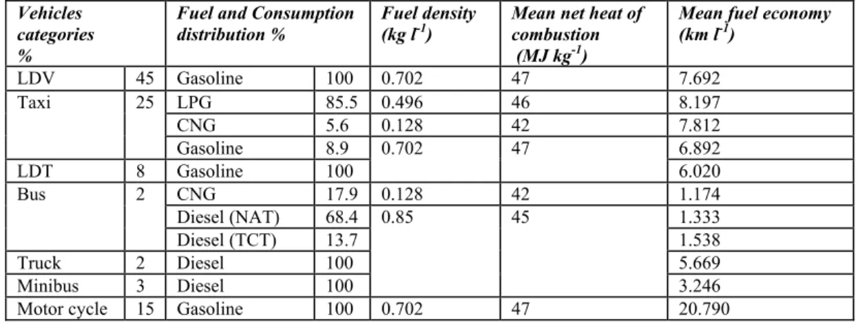
Regarding the vehicle categorizations presented in TERP project (1997), the data released by Tehran Traffic and Transportation Comprehensive Studies and vehicles registration data, the categorization presented in Table 2.2 was used to calculate emission factors.

2.2.1.1.2.2 Traffic data

In order to use the data received from TCTTS Co. and we adjusted the EMME2 outputs with actual fuel consumption. These actual consumption values were obtained from Ministry of Oil regarding the fuel consumptions. The reason for the difference between the consumptions rates of EMME2 and actual fuel consumption is due to the fact that the EMME2 network considers only the main roads of Tehran and ignores the secondary streets.

(35)

In order to calculate the emissions of all the vehicles, the vehicle kilometers traveled

(VKT) for each subcategory must be calculated. Figure 2.2 indicates the VKT for each

category. 0 5000 10000 15000 20000 25000

LDV LDT Taxi Motor Bus UCBT Buses MiniBus Truck M ill ions of VK T

Figure 2.2: VKT values across vehicle categories. Table 2.2: Categories & subcategories of Tehran vehicles.

Category of

Vehicles Subcategory of Vehicle Distribution

1- All of produced Paykan before of 1996 16.29

2- Imported Vehicle of older year 5.09

3- Other Iranian Produced Vehicle were produced before of 1995 8.15

4- LPG Converted Vehicle 1.22

5- Vehicle with Emission Standard of ECE 1503 31.57

6- Vehicle with Emission Standard of ECE 1504 16.29

7- Vehicle with Emission Standard of ECE R-8301 10.18

Light Duty Vehicle (LDV)

8- Vehicle with Emission Standard of ECE R-8303 11.21

1- All of LDT Produced before of 1995 52.43

2- light duty truck with emission standard of ECE 1503 20.39

3- light duty truck with emission standard of ECE 1504 7.77

4- light duty truck with emission standard of ECE R8301 13.59

Light Duty Truck (LDT)

5- light duty truck with emission standard of ECE R8303 5.83

1- Vehicle with the emission standard of ECE1504 6.00

2- LPG converted vehicle Taxi 85.00

Taxi

3- CNG converted vehicle 9.00

1- Mercedes Benz Minibuses & Minibuses with similar Technology 31.00

2- Fiat Minibuses & Minibuses with similar Technology Minibus 47.00

Minibus

3- IVECO Minibuses & Minibuses with similar Technology 22.00

1- Buses with Natural Aspirated Technology Non UBCT Bus 34.00

Non UCBT

Bus 2- Buses with Turbo charged Technology 66.00

1- Buses with Natural Aspirated Technology 80.00

2- Buses with Turbo charged Technology 11.00

3- LPG Converted Buses UBCT Bus 0

UBCT Bus

4- CNG Converted Buses 9.00

1- 4 Strock Motor cycle 50.00

2- 2 Strock Motor cycle 33.00

Motor Cycle

3- Mopeds 17.00

1- Trucks with Natural Aspirated Technology 74.00

Truck

(36)

2.2.1.1.3 Emission factors

In this study, in addition to the emission factors calculated in TERP report and the emission factors of COPERT III, the methodologies of Ntziachristos and Samaras, (2000) and Samaras et al. (1998) were used.

Based on this relative fraction of vehicles, aggregation emission factors and the fuel consumption rates were calculated.

2.2.1.1.4 On-Road emissions

The contribution of LDV vehicles was estimated to be close to 47% of total on-road emissions. LDT and motorcycles come next in terms of on-road emissions (see Figure 2.3). Figure 2.4 compares the estimations of on-road emissions in Tehran as presented in GEF project (1996), JICA (2002) and the current study for 2005.

0% 10% 20% 30% 40% 50% 60% 70% 80% 90% 100%

CO PM10 SO2 Nox NMVOC

P er ce n ta ge s of t o ta l Truck MiniBus UCBT Buses Bus Motor cycle Taxi LDT LDV

Figure 2.3: Comparison of each pollutant emission contribution to total

emissions across all categories.

0 20 40 60 80 100 120 140 160

CO SO2 NOx NMVOC PM10

10 00 t o nes (e xcpt f o r C O : 10, 00 0 t o n es) 1996 2002 2005

Figure 2.4: Comparison of results for on-road emissions of main

(37)

2.2.1.2 Railway emissions inventory

Using the fuel consumption data and accounting for both "HAUL" model (running model) and "YARD" model (maneuvering model), the average fuel economy was calculated for each rail road length. Finally, emission rates by trains in the GTA were calculated using the fuel consumption rates and the emission factors.

There are 3 main rail road lines in the GTA: 1. Tehran -Rey

2. Tehran - Aprin 3. Tehran -Lashkari

According to the data released from the JICA group regarding earthquake pathology (2000), the lengths of "HAUL" and "YARD" rail road lines are respectively 133 and 87 km. (These lengths include all the rail road lines).

The emission factors used here were obtained from the US Environmental Protection Agency (EPA) report (1992).

Since emission factors for some of the running locomotives were not available in the EPA report, emission factors from similar locomotives (band, model and power) were used here. Then, the emission factors of trains (both in running and maneuvering model) were calculated based on their locomotives model composition.

The emission rate of SO2depends on the sulfur content in the fuel. Since the locomotives

motors are equipped with the turbo charge system, the emission factors for SO2for heavy duty

vehicles were used for locomotives. The HAUL and YARD models from of the different types of trains are provided in Appendix A.

According to the Statistics and Technology Department of Rail Road of IRI, the fuel consumption rate by trains both in running and maneuvering status was exceeding 11930 and 1620 k liters respectively in 2005. Emissions from the trains are presented in Figure 2.5 for 2005.

(38)

0 200 400 600 800 1000 NOX SO2 CO HC PM10 To ne / y e a r Yard Haul

Figure 2.5: Pollutant emissions for rail road mobile sources.

2.2.1.3 Aircraft emission inventory

The contribution of airplanes which depart from or arrive at the Mehrabad international airport was estimated for 2005. Emissions are assigned to the landing strip and the flight route extended to both sides of the strip up to 1000 m height (landing – take off, (LTO) cycles). Airplanes are assumed to approach from the southwest and to take off and ascend toward the northwest (See Figure 2.6).

Figure 2.6: Considered cross section during taking off and ascending.

Total LTO emissions are obtained from those three lines and area sources extended around the landing strip.

The frequency of flights for each aircraft type is set based on the number of weekly flights for each company. Table 2.3 shows the weekly number of flights for each aircraft type. These aircraft types are recategorized into eleven types with engine specifications.

Table 2.3: Weekly frequency of flights from Mehrabad airport.

Type A-300 A-306 A-310 A-312 A-320

Number 80 15 10 4 2

Type B-707 B-727 B-72S B-734 B-737 B-747 B-74F B-74L B-763 B-767

Number 10 20 49 2 35 16 3 2 2 3

Type TU-134 TU-154 F-100 MD-11

Number 5 51 118 1 3° SE 5° NW Landing strip

(39)

An emission factor is assigned to each engine type and each LTO step. The duration of each step is: 4.0 sec (approach), 26.0 sec (idling), 0.8 sec (take off) and 1.6 sec (ascending). Then times are slightly different in the case of the F-100 type. The emission amount by step and air pollutant is summarized in Table 2.4. In actual calculation, emissions during the idling step are equally divided among three area sources. For diurnal profile, the same flight frequency is assumed except at nighttime. The emission release height for idling and take off is set at 10 m.

Table 2.4: Total emission from airplanes.

Step / element CO SOx NOx

Approach 0.63 0.45 4.79

Idling 182.15 0.97 3.94

Take off 0.34 0.29 10.18

climb 1.18 0.50 13.31

2.2.2 Stationary emissions inventory survey

The stationary point and area source emissions were originally estimated from a mail survey source registration. Activity data include the quantity and type of fuel used and also in some case fuel sales records, state registration records, fuel/material usage and default employment and per capita data. The emission factors are based on source classification codes related to the source process type. If control equipment is used at any source, its effectiveness is factored into the equation. Field staff also supplemented data based on plant inspections and manually calculated plant emissions.

Brief descriptions of the categories for projecting pollutants are shown in Table 2.5. By study of activity factors such as sector-wise energy demand, emission factors of fuels, emission rates of pollutants were estimated for each sector in Tehran. Table 2.6 shows sectorwise stationary emission quantities of pollutants in Tehran during 2005.

Table 2.5: Brief descriptions of the categories for stationary sources.

Sector Category Emission Type

Manufacturing

Industry Food, Textile, Wood, Paper, Chemicals, Nonmetal, Iron/Steel, Machinery, Other Point (>100 employee) Area (<100 employee)

Commercial

Household Restaurant, Hotel, Office, House, etc. Area Energy

Conversion

(40)

Table 2.6: Sectorwise emission quantities by stationary sources

in Tehran during 2005 (combustion + evaporation) tone/year.

Emission quantity Sector

SOx NOx CO HC SPM Industry 15923 5741 1309 5748 3568

General service and household 17720 30051 7893 38347 8591

Energy conversation 9289 12014 2053 9401 2838

Total 42932 47806 11255 53496 14997

2.2.3 Results and discussion

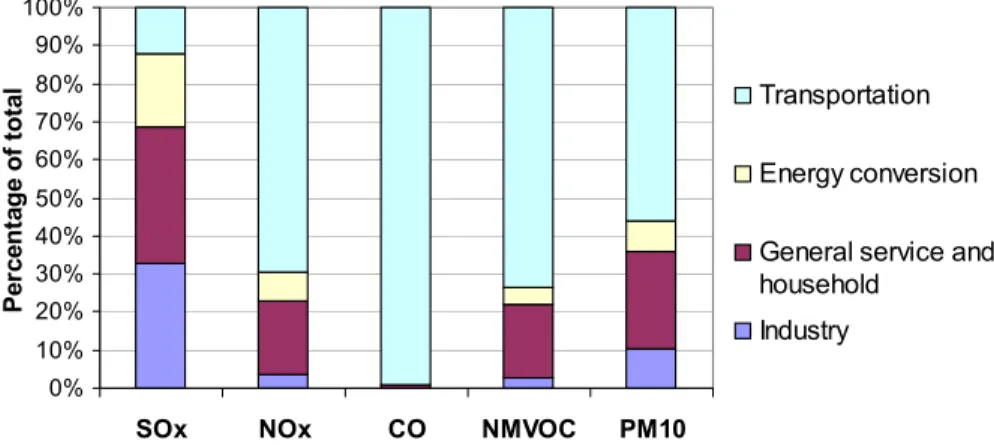
Concerning the source contribution of air pollutants, stationary sources represent 87% of total SOx emission while mobile sources represent respectively 70%, 99%, 72% and 56% of NOx, CO, NMVOC and PM10 emissions respectively (See Figure 2.7).

0% 10% 20% 30% 40% 50% 60% 70% 80% 90% 100%

SOx NOx CO NMVOC PM10

P er ce n ta g e o f to ta l _{Transportation} Energy conversion General service and household

Industry

Figure 2.7: Comparison of air pollutant emission contributions to total across main sectors.

SOx emissions from the general service and household represent 36% of the total, followed by the industrial sector (32%), energy conversion (19%), while the transportation sector represents only 13% in contrast to other kinds of pollutant emissions, because this sector uses low sulfur gasoline and diesel oil. The thermal power plants and refinery in Tehran contributions is only 19% because most of the fuels have already been substituted by natural gas expect in winter when supply of natural gas is sometimes short. NOx emission shows different treatment to SOx and the contribution of the transportation sector reaches 70% of total emissions. General service and household and energy conversation contribute 19% and 8% respectively, followed by industrial (4%). The general service and household sector contribution is 18%, though this sector has numerous consuming units. CO emissions are negligible in the case of stationary emission

(41)

sources, since the transportation sector has a dominant contribution of 99%. Most NMVOC emissions come from the transportation sector with 72%, general service and household (19%) and energy conversion (5%); the combined share of these three sectors totals 97%. NMVOC emission sources of the commercial sector are represented by petrol stations, printing shops, dry cleaning shops and petroleum depots and not by shops of electric metal plating and painting, since information of these sources is not available despite their possible substantial volume. It is estimated that leakage of natural gas from rubber hose connections is substantial due to a lack of proper maintenance, especially in the commercial-household sector although their volume is not estimated at this stage. PM10 emissions from the transportation sector represent 56% of the total, followed by general service and household (25%) and the industrial sector (10%) and energy conversion (8%).

Figure 2.8 illustrates hourly average of CO and PM10 emission inventories during 2005, these pollutants are the two critical pollutants in Tehran city.

Figure 2.8: Hourly average of CO (left) and PM 10 (right) emission inventories for Tehran city during 2005

(42)

2.3 Emission inventory of anthropogenic heating in Tehran 2.3.1 Overview

The heat generation due to human activities is an important cause of the urban heat island (Oke, 1998). The heat island of some mega-cities have been documented by investigating extensive direct and remote sensing measurements as well as simulation studies, such as urban parameterizations in mesoscale meteorological and fluid dynamics models (Kim, 1992; Aniello et al., 1995; Ichinose et al., 1999; Saaroni et al., 2000; Martilli, 2002; Kondo and Kikegawa, 2003; Kato and Yamaguchi, 2005; Hung et al., 2006).

One of the main goals of this study is to estimate diurnal profile and distribution of anthropogenic heat flux (Qf) in Tehran city, including a detailed formulation of this flux in a high resolution mesoscale meteorological (MM) model of the urban environment. In the past decade, parameterization schemes such as Canopy Models (CM), Building Energy Models (BEM), the Drag-force Approach (DA) and urban soil models have been implemented in MM models to better incorporate urban geometric structure and thermodynamic characteristics. Therefore, new generations of MM models (see Figure 2.9) have multi-scale systems (MM–CM–BEM) that can be used for the quantitative assessment of the urban island effect. Similarly, this kind of parameterizations can be incorporated into Computational Fluid Dynamics (CFD) models (Milliez et al., 2006).

(43)

Formulations for Qf or its components have been introduced into standard and modified versions of MM models (MM–CM or MM–CM–BEM) to study anthropogenic heating effects on local meteorology (Sailor et al, 2006; Martilli et al, 2002; Kikegawa et al, 2003).

Recent studies show daily average value of Qf in the range of 25 to 50 Wm-2 and with maxima up to about 80 Wm-2 in city-scale analyses (Klysik, 1996; Steinecke, 1999; Crutzen, 2004; Sailor and Lu, 2004; Offerrle, 2005; Piringer and Joffer, 2005; Makar et al., 2006; Pigeon et al., 2006; Pigeon et al., 2007; Hamilton et al., 2009), while results with high spatial resolution in the downtown areas of mega-cities (e.g. Tokyo, San Francisco and Shenyang) show 5–10 times the magnitude of the city-scale average values (Saitoh and Shimada, 1996; Ichinose et al., 1999; Sang et al., 2000; Sailor and Lu, 2004). All recent studies confirm significant effects of anthropogenic heating on the formation of UHI and account for this flux in the urban energy balance. Taking into account Qf in MM models of mega-cities usually increases the simulated near-surface temperature by 0.5-5°C (Saitoh and Shimada, 1996; Ichinose et al., 1999; Kondo and Kikegawa, 2003; Kikegawa et al, 2003; Sailor and Fan, 2004, Makar et al., 2006; Sailor et al., 2006). The spatial distribution of Qf is not easily available from monitoring data and is difficult to obtain from measurements and energy consumption inventory (Pigeon et al., 2006). Consequently, it has generally been difficult to estimate the spatial distribution of Qf and correctly estimate both heat storage and Qf in modeling studies (Pigeon et al., 2006; Offerle et al., 2005). The general calculating methods for spatial distribution of Qf can be based on some available relevant urban characteristics, such as meteorological measurements (Pigeon et al., 2006), population density pattern (Sailor and Lu, 2004; Markar et al., 2006), brightness (based on satellite images) (Makar et al., 2006), landuse classification (Piringer and Joffre, 2005), emission inventory for specific pollutants and measured or simulated fields of specific pollutant concentration ( Baklanov, 2005). This work presents the design and application of a suitable method to develop spatial and temporal distributions of Qf in mega-cites.

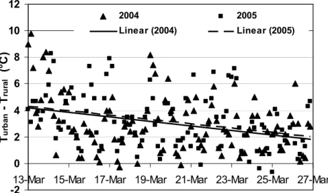
The analysis of meteorological data from the Tehran observation network in urban, suburban and rural areas shows UHI intensity being stronger in winter, especially at night