Anisothermal cyclic plasticity modelling of martensitic steels

HAL Id: hal-01715087

https://hal.archives-ouvertes.fr/hal-01715087

Submitted on 11 Jan 2019

HAL is a multi-disciplinary open access archive for the deposit and dissemination of sci-entific research documents, whether they are pub-lished or not. The documents may come from teaching and research institutions in France or abroad, or from public or private research centers.

L’archive ouverte pluridisciplinaire HAL, est destinée au dépôt et à la diffusion de documents scientifiques de niveau recherche, publiés ou non, émanant des établissements d’enseignement et de recherche français ou étrangers, des laboratoires publics ou privés.

Anisothermal cyclic plasticity modelling of martensitic

steels

Z Zhang, Denis Delagnes, Gérard Bernhart

To cite this version:

Z Zhang, Denis Delagnes, Gérard Bernhart. Anisothermal cyclic plasticity modelling of marten-sitic steels. International Journal of Fatigue, Elsevier, 2002, 24 (6), pp.635-648. �10.1016/S0142-1123(01)00182-7�. �hal-01715087�

Anisothermal cyclic plasticity modelling of martensitic steels

Z. Zhang

_{, D. Delagnes}

_{, G. Bernhart}

a_{Research Centre on Tools, Materials and Processes (CROMeP), Ecole des Mines d’Albi-Carmaux, 81013 Albi, CT cedex 09, France} b_{Institute of Metal and Technology, Dalian Maritime University, Dalian 116026, China}

Abstract

Tempered martensitic steels were investigated in isothermal and thermomechanical fatigue conditions and general features of their cyclic behaviour are reported. A cyclic anisothermal constitutive model with internal variables was formulated to describe their behaviour; it allows the description of the Baushinger effect, the continuous cyclic softening, the strain rate dependence and the plastic strain memorisation. When compared to experimental results, isothermal and anisothermal model predictions show good coherence. This model is helpful to understand and explain some experimental results such as the increase in strain softening when strain rate decreases in isothermal testing, as well as the relations between mean stress and temperature range or cyclic softening with strain amplitude in anisothermal conditions.

Keywords: Thermomechanical fatigue; Martensitic steel; Cyclic softening; Stress–strain modelling; Plasticity

1. Introduction

Fatigue behaviour of austenitic stainless steels has been widely investigated during the last 25 years since experimental facilities to perform fatigue tests in total or plastic strain control have been in general use, hence the prolific literature available [1–3]. Conversely, fatigue properties of tempered martensitic or bainitic steels are not so well known. First, the major part of the results are still confidential and so have not been published. Indeed, martensitic or bainitic steels are generally used for their good mechanical strength at high temperatures associa-ted with sufficient ductility for the power generation industry (steam turbine blades, first wall of fusion reac-tors, parts subjected to stresses at high temperature), the petrochemical industry, and also for tools in areas of strong economic competition. Secondly, the heat treat-ment which consists in annealing, austenitising, quench-ing and one or two temperquench-ing operations leads to a com-plex microstructure which is rather far from pure or binary alloys generally investigated (mainly f.c.c. structures) where mechanisms of cyclic plasticity can be

* Corresponding author. Tel: +33-(0)5-63-49-30-56 http://www.enstimac.fr.

E-mail address: bernhart@enstimac.fr (G. Bernhart).

well understood and explained using TEM obser-vations [4,5].

Microstructure of low or medium carbon steels is made of thin laths (their width can be less than 0.1 µm). Inside the laths, the high dislocation density generated during the quench, associated with a fine carbide precipi-tation occurring during tempering, is responsible for investigation difficulties. Although some interpretations of martensitic steels cyclic plasticity mechanisms have been carried out [6–11], quantitative evaluation of rel-evant microstructure parameters which are responsible for good fatigue resistance at high temperatures is not so frequently encountered (carbide density and mor-phology, carbide chemical composition, dislocation den-sity, lath size, etc.). It is nevertheless essential to control the evolution of these parameters with temperature, time and strain amplitude in order to take into account the fatigue resistance in the definition of the heat treatment conditions, because fatigue is the usual manner of in-service tool steel degradation. The ultimate aim of such an approach, which consists in understanding interac-tions between microstructure and properties, is to ensure a good prediction of fatigue behaviour to optimise tool conception and to derive a more realistic life predic-tion model.

In parallel to the research for micro-structural under-standing, optimisation of tool design through numerical

finite element calculation needs constitutive models able to describe accurately the macroscopic behaviour. Uni-fied elasto-viscoplastic phenomenological models based on internal state variables are the most popular to reach these goal. Numerous authors have published such mod-els and these may be divided in two categories: micro-structure related models taking into account explicitly parameters like dislocation densities, grain sizes, etc. as those published by Estrin [12], and physical-phenomel-ogical models for which each phenomena is described with a corresponding state variable [13–17]. Amongst them, the Miller MATMOD4 model [13] and the Chaboche model [14] are well known; they differ princi-pally in the way they take into account the temperature, i.e. only in the strain rate equations for the first one, whereas in most other models, state variable parameters may all be temperature dependant. The last one is also developed in the framework of the thermodynamics of irreversible processes and was chosen as the basis of the present work.

In a first work [18] an elasto-plastic non-linear kinem-atic and isotropic hardening model was derived which is able to reproduce quite well the experimental behaviour. In that work, the basic formulation was adapted to mar-tensitic steels to integrate the continuous softening observed on martensitic or bainitic steels.

As tools are generally subjected to numerous severe mechanical and thermal loads, it is of great importance to derive an anisothermal constitutive model which is able to take into account the great range of strain rates as well as the temperature variations.

After a recall of the main characteristics of isothermal fatigue behaviour of martensitic steels, results of thermo-mechanical fatigue tests are presented in the first part. The general formulation of a kinematic non-linear and isotropic thermo-elasto-viscoplastic model able to describe the complex cyclic behaviour is presented in the second part. The model is validated in the last part by comparing predictions and experimental obser-vations.

2. Experimental fatigue behaviour of martensitic steels

2.1. Isothermal fatigue behaviour

Two tempered martensitic hot working tool steels (X38CrMoV5 (AISI H11), 55NiCrMoV7 (EN 10027-1)) have been extensively investigated in isothermal fatigue conditions [19,18]. The most important aspects of their behaviour are discussed below.

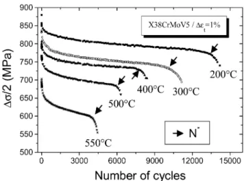
Fig. 1 shows the half stress amplitude versus the num-ber of cycles at several temperatures for the 5%Cr steel and a total strain amplitude of 1%. All the curves can be divided into three different parts: a strong softening

Fig. 1. Cyclic softening of a X38CrMoV5 (AISI H11) tempered mar-tensitic steel.

is observed during the first few hundreds of cycles, fol-lowed by a slow steady softening during the major part of the life, and finally, propagation of one or several cracks in the specimen gauge length induces the drastic decrease of the stress amplitude just before the specimen rupture. It was shown [19] that the first and the second parts were not associated with crack propagation but rather they are closely connected to microstructure evol-utions. So, martensitic or bainitic steels exhibit a con-tinuous softening from the first cycle till rupture; this is a typical fatigue behaviour more complex to understand and to model than the major part of the metallic materials investigated which stabilise after a few tens or hundreds of cycles.

Cyclic softening is generally explained by the modi-fication of dislocation structure and density and/or car-bide morphology, chemical composition and density. First, the tangle of dislocations is gradually crushed and dislocation cells begin to form after several cycles [6– 10]. Dislocation density becomes very heterogeneous with a strongly reduced density inside the cells. Such a configuration promotes free motion of the dislocations between the walls, and free slip distances are increased. However, dislocation cell formation is not the sole mechanism. Indeed, when lathes are very thin, the annihilation of dislocations occurs by cross-slip of screw dislocations and the climb of edge dislocations at high temperatures. Thus, a strong reduction of dislocation density is observed without any cell formation. Next, at high temperatures, carbide coalescence takes place inducing a loss of their density and consequently the dis-location mean free path increases. Moreover, the mor-phology of very elongated platelets, probably due to a crystallographic coherence with the matrix, is modified to obtain a more globular shape [11,19,20]. These mech-anisms also contribute to cyclic softening promoting

dis-location mobility and reducing the steel resistance due to the fine precipitation occurring during tempering. The total softening amplitude, D, was defined [19] by the following equation:

D!

!

2

"

#

!

"

(1) where N*_{is the last cycle located in the second part (see}

Fig. 1) just before the loss of stress amplitude mainly due to macroscopic crack propagation

Temperature is of course the first parameter that influences the softening amplitude and kinetics as shown in Fig. 1. Fig. 2 shows that the total softening amplitude also strongly depends on total strain amplitude. Satu-ration of D for the highest "et of the experimental

pro-gramme has also been observed. At 300°C, the total softening amplitude reaches 170 MPa, which represents nearly 20% of the stress amplitude recorded during the first cycle. Similar dependence of softening with the initial strain amplitude was also found for the 55NiCrMoV7 steel [21]. Consequently, this strong softening effect should be taken into account to obtain a realistic stress distribution of in-service tool.

For a given total or plastic strain amplitude, a decrease of the total softening amplitude has been observed for the 5%Cr hot work tool steel when the hardness level is increased (see Figs. 3 and 4). In other words, the steel tends to become more stable. This better cyclic stability may result from higher dislocation and carbide density generally observed in the initial state that decreases dis-location mobility preventing cell formation or dislo-cation annihilation.

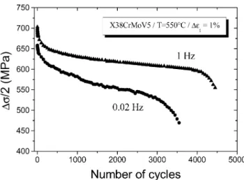
Another significant parameter is the fatigue testing frequency. Indeed, viscous effects became important at relatively high temperatures, i.e. around normal service conditions (generally between 500°C and 700°C for pressure casting dies for light alloy injection, forging

Fig. 2. Influence of total strain amplitude on softening amplitude (AISI H11 at 300°C).

Fig. 3. Cyclic softening for two different hardness of a H11 steel at 550°C.

Fig. 4. Hardness influence on softening amplitude.

moulds, extrusion tools, etc.). Fig. 5 illustrates this strain rate effect: when testing frequency is decreased from 1 Hz to 0.01 Hz, a variation of important mechanical characteristics such as the “true” yield stress, plastic strain amplitude per cycle, softening amplitude and rate is introduced.

2.2. Thermo-mechanical fatigue (TMF) behaviour

Thermo-mechanical fatigue behaviour of a 47 HRc (Rockwell hardness) 55NiCrMoV7 martensitic tool steel was investigated in the range 300–500°C. A more detailed description of the tool steel composition, heat treatment and structure can be found in [18]. The objec-tive of these TMF tests [22] is to gather hystheresis loops over a few hundreds of cycles to support the validation of the anisothermal constitutive model.

Fig. 5. Strain rate effect on the cyclic softening.

2.2.1. Experimental procedure and test program

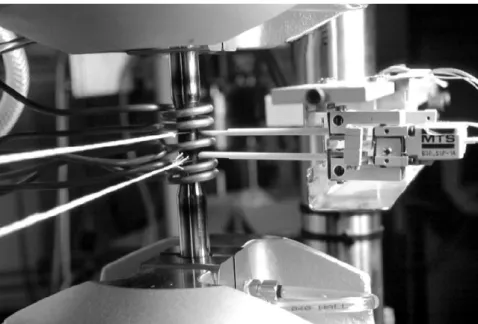
The TMF tests were carried out with a closed-loop 810 MTS servo-hydraulic testing machine and Teststar II _{controller connected to a personal computer. The}

complete experimental set up is presented in Fig. 6. A smooth shank, thin walled tube (wall thickness of 1 mm) specimen was designed. It was mounted in water-cooled hydraulic wedge grips for conduction cooling.

Heating was achieved with a 6 kW induction gener-ator and a three zone coil configuration shown in Fig. 7 (two main coils located at the top and bottom of the gauge length and a minor coil at mid point). During the designing stage of the coil, continuous monitoring of temperature was performed with three Type K thermo-couples located at mid zone and 7 mm on either side. Before applying the thermocouples mechanically to the specimen with springs, the two wires were flattened and spot welded against each other. During testing only two

Fig. 6. TMF experimental test equipment.

thermocouples were used (Fig. 7); the upper one was used as a feedback sensor to an Eurotherm closed loop temperature control system. It was also used to change the setpoints of the temperature controller through an RS232 link to the computer when necessary. During thermal cycling in the range of 300–500°C at a rate of 200°C/min, the maximal thermal gradient recorded over the 12 mm gauge length of the high temperature exten-someter was lower than 10°C in axial and radial direc-tions. Most of the experimental features related to the thermal behaviour of the samples reported by Castelli et al. [23] were confirmed during the preparatory phase of the test program.

The tests were performed under a constant mechanical strain rate (e˙m=constant). Providing that the thermal

amplitude and rate was kept constant (200°C in 60 s), mechanical strain rates ranged from 1.6×10#4 _s#1 _to

5×10#4_s#1_{. Real time thermal strain compensation was}

achieved using a linear thermal strain (eth) temperature

relationship in the formeth=lT+m. Coefficients l and m

were determined during thermal cycling under zero load prior to the test campaign (if necessary they may be cor-rected before each test).

The test-control program was developed using the Testware _{macro-language software supplied by MTS.}

It uses the real-time and the “Calculated Entry” capabili-ties of the Teststar II _{controller. Thus the mechanical}

strain is calculated (and updated with a frequency of 3 kHz) with the relation:

em!et#eth (2)

whereetis the total strain measured by the extensometer

andethis the real time calculated thermal strain with the

upper thermocouple temperature input value. Closed loop strain rate control is performed using the calculated mechanical strain input signal.

Fig. 7. Induction coil, extensometer and thermocouples.

The mechanical strain and temperature triangular sig-nals are phased in such a way that the mechanical strain reverses the temperature control setpoints when maximum or minimum mechanical strain levels are reached. To minimise the thermal gradients at strain reversal due to the thermal inertia of the system, the tem-perature rate setpoint is lowered to a value of 50°C/min, 5°C before the final temperature is reached.

Three types of TMF tests were conducted: In-Phase (IP) test (maximum strain occurs at maximum temperature), Out-of-Phase (OP) tests (maximum strain at minimum temperature) and Out-of-Phase Compress-ive (OPC) tests (maximum strain at minimum tempera-ture and only compressive strains). This last test was introduced as it is closest to the type of TMF cycling of the surface of a hot forging or casting tool. An iso-thermal test was also performed at 500°C. The whole test program is summarised in Table 1.

After 10 thermal cycles under zero load to reach dynamic thermal stabilisation, the test proceeds with a first mechanical cycle performed by decreasing the mechanical strain from zero strain at 400°C for the IP and OP tests, and from zero strain at 300°C for the OPC

Table 1 TMF test program IP 300– OP 300– OPC 300– ISO 500°C _{500°C 500°C 500°C} em min/em max _{#0.7/+0.7 #0.7/+0.7 #0.7/+0.7} (%/%) #1/+1 #1/+1 #1/0 #1.25/+1.25 #1.25/+1.25 #1.25/0 #1.5/+1.5

tests. Stress, mechanical strain, temperature, time values were recorded all 10 cycles; the same was done for the stresses at maximum and minimum mechanical strains for all cycles.

2.2.2. Test results

Fig. 8(a) shows the tenth fatigue loop of three samples tested in the same mechanical strain range (#0.7%/+0.7%) and strain rate, but in three different temperature conditions: isothermal condition at 500°C (ISO 500), temperature variation between 300°C and 500°C In-Phase (IP 300–500) and Out-of-Phase (OP 300–500). It can be seen that anisothermal loops are asymmetrical when compared to isothermal ones. The higher stress (in absolute value) is always reached for the lower temperature 300°C and is either tensile or compressive. For this low mechanical strain amplitude IP and the OP loops look very similar, and OP loop is shifted to higher stress levels. The isothermal loop comes quite close to the values of the anisothermal ones for the temperatures near 500°C. This latter loop is sym-metrical and shows a greater plastic strain amplitude. This is confirmed in the stress–plastic strain plots [Fig. 8(b)]: IP TMF and OP TMF tests show similar plastic strain amplitude ranges, lower than isothermal strain amplitudes at 500°C. Nevertheless the loops are in the compressive strain range for OP tests whereas they are in the positive strain range for IP tests.

Due to the asymmetry of anisothermal loops, the mean stress is positive for OP cycling, and negative for IP cycling. This is a typical result in TMF testing and was also reported for other classes of materials [24–26]. Fig. 9 shows the mean stress evolution of all the TMF tests: all IP tests (respectively OP tests) show the same com-pressive stress #280 MPa (respectively tensile stress

Fig. 8. 55NiCrMoV7 10th TMF hysteresis loop: "em =1.4%,

iso-thermal cycling 500°C, IP cycling 300–500°C, OP cycling 300–500°C. (a) Stress–mechanical strain loops, (b) stress–plastic strain loops.

Fig. 9. Mean stress versus number of cycles in TMF tests.

+200 MPa). Even the OPC tests gives the same result (see Section 4.2 for more discussion). It may be con-cluded that the mean stress in TMF tests is only related to the temperature range and the type of test—IP or OP (including the OPC)—whatever the mechanical strain range. These values are symmetrical about the mean stress of #40 MPa, measured for the isothermal tests. Such a low compressive mean stress for isothermal sym-metrical total strain fatigue tests was always observed

during martensitic steel testing whatever the material, the temperature and the strain amplitude [18,19].

3. Anisothermal cyclic plasticity model

3.1. Theoretical background

The anisothermal cyclic model is formulated within the theoretical framework of the thermodynamics of irre-versible processes. This theory [27] assumes that the evolution of a material system can be described as a suc-cession of equilibrium states. It introduces two sets of variables, the observables (like total strain, temperature) and the internal variables so as to define completely a material element and its evolution over time and tem-perature.

In the classical unified visco-plastic theory with internal variables [28] the deformation is divided into an elastic and plastic part, and the cyclic behaviour is completely defined by two internal stress variables and associated evolution rules. At this point it is important to notice that experimental observations reported in the previous paragraph have been taken into account to make an appropriate choice for the expressions of internal stress variables.

As usual [14] two stress variables X¯¯ (tensorial) and

R (scalar) are introduced to describe the non-linear

kine-matic hardening and the isotropic hardening.

3.1.1. Anisothermal non-linear kinematic hardening

The back stress X¯¯1 _{is linearly related to an internal}

strain variable a¯¯ which characterises the internal strain misfit coming from the plastic straining [29] in the form:

X¯¯!2

3a(T)c(T)a¯¯ (3)

where a(T) and c(T) are two material parameters depending only on temperature. As has been shown in previous work [18] kinematic hardening of martensitic steel undergoes no changes during cycling. The expression of the evolution rule of a¯¯ in the form a

!_{˙ #e!˙}

p#c(T)a¯¯p˙ (4)

proposed by Armstrong and Fredericks [30] introduces the evanescent strain memory during each cycle respon-sible for the Baushinger effects.

Thus the anisothermal non linear kinematic hardening stress evolution rule is in the form [31]

X !_{˙ !c(T)}

!

"

!

1 _{u¯¯ tensorial stress or strain variable, u}=˙ tensorial stress or strain

$ 1

a(T)

∂a(T)

∂T

"

3.1.2. Anisothermal isotropic hardening

To take into account the non saturating cyclic soften-ing observed experimentally (Fig. 1 and [18]), the drag stress R is divided into two stresses R1 and R2 linearly

related to two internal variables r1 and r2:

R1!Q1(T)·r1 (6)

R2!b(T)·Q2(q,T)·r2 (7)

where Q1(T) and b(T) are two material parameters

depending only on the temperature, and Q2(q,T) is

defined in the next paragraph.

Evolution rules for the internal variables are as fol-lows:

r˙1!p˙ (8)

r˙2!p˙·(1#b(T)·r2) (9)

where p is the cumulative plastic strain (p˙=√2/3e=˙p:e=˙p).

If the physical meaning of the back stress R2,

corre-sponding to the initial exponential softening, can be related to the rapid reduction of high dislocation density induced by quenching as explained in Section 2.1, the mechanism responsible for the linear non saturating softening, through back stress R1is not yet clearly

ident-ified. As it appears also at room temperature, mech-anisms such as slow saturation of dislocation density reduction, formation of dislocation cells, interaction with lath boundaries or carbide morphology or density evol-ution may be put forward.

The anisothermal isotropic hardening rule is thus defined by: R˙1!Q1(T)·r˙1$r1· ∂Q1(T) ∂T ·T˙ (10) R˙2!b(T)·Q2(q,T)·r˙$r2·

!

"

After substitution of Eqs. (8) and (9) into Eqs. (10) and (11), back stress evolution can be written:

R˙1!Q1(T)·p˙$R1· 1 Q1(T) ·∂Q1(T) ∂T ·T˙ (12) R˙2!b(T)·(Q2(q,T)#R2)·p˙$R2·

!

"

The visco-plastic strain evolution is defined as2

p˙!

#

$

n(T)

(14) where G=J2(X¯¯#s¯¯)#R1(T,p)#R2(T,p)#k(T) defines a

Von Mises type yield surface, K(T), n(T), k(T) are temperature and material dependent parameters and

J2(X¯¯#s¯¯)=√3/2(X¯¯%−s¯¯%):(X¯¯%−s¯¯%) with X¯¯% and s¯¯% the

deviatoric parts of X¯¯ and s¯¯.

Under isothermal conditions (i.e. T˙=0), Eqs. (12) and (13) simplify to:

R˙!R˙1$R˙2!Q1(T)·p˙$b(T)·(Q2(q,T)#R2)·p˙ (15)

which can be rewritten in the particular form given in reference [18]:

R˙!Q1(T)·p˙$b(T)·(Q1(T)·p$Q2(q,T)#R)·p˙ (16)

and whose integration leads to equation

R(p,T)!Q1(T)p$Q2(q,T)(1#exp(#b(T)·p)). (17)

This last equation shows the linear and exponential parts of the cyclic softening.

3.1.3. Plastic strain memorisation

Experimental observations reported in Section 1 for martensitic steels give evidence of the softening depen-dence on initial plastic strain level. Internal variables that memorise the prior maximum plastic strain range have to be introduced in the model [14]. They use the memory surface in the plastic strain space first proposed by Ohno [32]:

F!2

3J2(e¯¯p#x¯¯)#q. (18) As illustrated in Fig. 10, for an uniaxial non symmetrical

Fig. 10. Schematics of the strain memory variable meaning in the non symmetric tensile–compressive configuration.

2 _{%u&=u if u&0 and %u&=0 if u'0; sign(u)=+1 if u(0 and}

tension-compression configuration, x¯¯ represents the centre of the memory surface and q its radius in the strain space.

Plastic flow inside the strain domain (i.e. F'0) does not change the “memory state”. Evolution rules for q andx¯¯ are: q˙!h%n¯¯:n¯¯∗_{&p˙ (19)} x !˙ !3 2(1#h)%n¯¯:n¯¯∗&n¯¯∗p˙ (20) where n¯¯ and n¯¯∗_{are respectively the units normal to the}

yield surface G=0 and the memory surface F=0. Ohno introduces the constanth to induce a progressive mem-orisation and a value of1

2may be used in reversed cyclic

conditions for instantaneous memorisation. This plastic strain memorisation is used in the isotropic softening variable [Eq. (5)] and it was shown previously [18] that the particular form

Q2(q,T)!Q2)(T)·(1#exp(#2mq)) (21)

may be used for martensitic steels.

3.2. Unidirectional cyclic plasticity model for martensitic steels

In the unidirectional tensile-compressive conditions where cycling is performed under mechanical strain amplitude and temperature changes (like the experi-mental TMF tests reported previously), the model sim-plifies to the following set of equations when introducing two kinematic variables Xi (i=1,2) to allow the

simul-ation of the experimental behaviour: s!E(T)(em#ep) p˙!

#

$

!

"

q˙=hp˙%sign(s−*Xi)(ep−x)&

x˙=(1−h)p˙%sign(s−*Xi)(ep−x)& sign(ep−x)

'

if |ep#x|#q

&0

q˙!0 and x˙!0 if |ep#x|#q'0

where E (Young’s modulus), ai, ci, b, Q1, Q2), K, k are

material and temperature dependent parameters. A numerical computer program (TEVP; Thermo-Ela-sto-Visco-Plastic) was written in Fortran to integrate this set of differential equations. Hence, experimental results and numerical predictions could be easily compared, providing the model parameters are known.

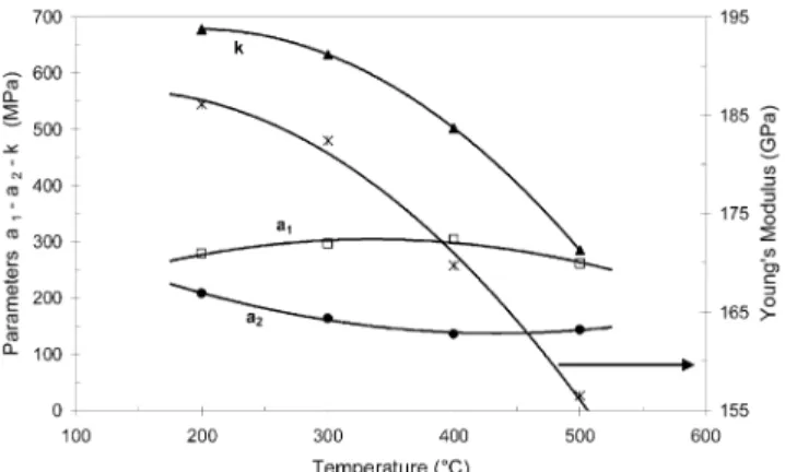
Fig. 11. Isotropic hardening parameter evolution with temperature.

3.3. Model parameter identification

Model parameters were identified for the 55NiCrMoV7 steel in the 200–500°C temperature range where the material could be considered to be in structural stability for short test durations due to the tempering treatment performed at 510°C. Reversed isothermal fatigue tests at various total strain amplitudes and mono-tonic tests at different strain rates were conducted. The former are presented in more detail in [18] where para-meters related to the isotropic stress variable R can be found.

To take into account the viscous stress, monotonic tests at 10#2_s#1_{, 10}#3 _s#1_{and 10}#4_s#1 _{total strain rate}

were conducted. The whole set of parameters was ident-ified after successive iterations using Excel _and

Mat-lab_{numerical tools [21]. Figs. 11 and 12 show the}

evol-ution of some of these parameters with temperature; isotropic parameters Q1 and b vary linearly when the

temperature increases, whereas the kinematic parameters

a1 and a2, as well as Young’s modulus and the strain

rate independent initial elastic stress k show quadratic evolution. In comparison to values reported in [18] for the elasto-plastic model, values of k are much lower. The difference between the two sets of values is related to

the contribution of the viscous stress (Ke˙1/n

p ). As a result

of this identification process, the evolution of each model parameter (10 parameters) can be fitted by an ana-lytical curve which is used in the TEVP program to determine the parameter value and its derivatives at each time and temperature increment. Linear or quadratic fit-tings for the parameters were used as shown in Figs. 11 and 12.

Nevertheless it should be mentioned that such an identification process is costly and time consuming. Thus an optimised combined experimental and Matlab

identification procedure was developed to simplify this task. It is applicable to materials having similar behav-iours such as martensitic steels, and it is based on a sin-gle specimen test per temperature to obtain all the para-meters of the model [33].

4. Isothermal and anisothermal model results and discussion

4.1. Isothermal model results

The isothermal model was checked by comparing a non symmetrical (#0.5/+1%) total strain controlled fatigue test with the simulation results. Fig. 13 shows the

Fig. 13. Non symmetrical total strain (#0.5/1%) fatigue test at 500°C. Stress–plastic strain loops 1, 5, 10, 50, 100, 500, 1000. (a) Experimental, (b) model response.

stress–total strain response and the stress–plastic strain responses. The model reproduces each experimental fea-ture well: Bauschinger effect, mean stress relaxation, plastic strain shifting to the positive plastic strain range and increase of the plastic strain amplitude (after stress relaxation) due to isotropic softening.

Fig. 14 illustrates the change of the hysteresis loop during an isothermal symmetrical fatigue test simulation when strain rate varies. It can be seen at 500°C, which corresponds to a near service temperature of martensitic tool steels, that loading rate has an important effect on the behaviour. For example the stress at a plastic strain of 0.2% drops from 920 MPa at 10#2_s#1 _(which

corre-sponds to mechanical forging) to 780 MPa at 10#4 _s#1

(for typical hydraulic forging). Consequently it may sometimes be wrong to use conventional material properties available in data bases or norms in order to design a die, without taking into account the accurate service loading rate.

This modelling allows also an explanation of the increase of the softening rate when decreasing the testing frequency as reported previously in Section 1.2. Evol-ution of the predicted semi-stress amplitude is plotted in Fig. 15 with respect to the number of cycles (a), and the cumulated plastic strain p (b). It is observed in Fig. 15(a) that the same trends as the experimental ones are found, i.e. when the strain rate decreases from 10#2_s#1_{to 10}#5

s#1_{, the softening rate increases when considering the}

steady softening range. But this is only an apparent increase resulting from the representation in a plot related to the number of cycles. As a matter of fact, the plot on Fig. 15(b), which is related to the model formu-lation through the cumulated plastic strain p, shows the same softening rate whatever the strain rate. But as the plastic strain amplitude during one cycle is greater at low strain rate (as shown in Fig. 14), the cumulated plas-tic strain also becomes greater; for example after 500 cycles the cumulated plastic strain p is 6.5 for 10#4_s#1_,

and only 5.15 for 10#2 _s#1_{. So it can be stated that the}

Fig. 14. 10th stress plastic strain loop at 500°C and "et=1.6% for

Fig. 15. 55NiCrMoV7; Calculated semi-stress amplitude at 500°C and "et=1.6% for different total strain rates. (a) Semi-stress amplitude

versus number of cycles, (b) semi-stress amplitude versus cumulated plastic strain.

softening rate increase during testing at lower fre-quencies is not a feature of the material.

4.2. Anisothermal model results and discussion

Anisothermal model formulation allows the simul-ation of the TMF tests presented in Section 2.2. Fig. 16 compares the model response obtained with the TEVP program for the 10th cycle of a mechanical strain con-trolled test in the range #0.7/+0.7% for the isothermal conditions at 500°C and 300°C with those for the IP and OP 300–500°C conditions. In such conditions, results are similar to the experimental ones of Fig. 8. The absolute maximum stress is always observed for the lowest tem-perature (300°C); the isothermal responses at 500°C and 300°C have the same maximum and minimum stresses as those calculated for the anisothermal conditions at the same temperatures. IP test simulation shows positive plastic strain cycling whereas OP induces plastic cycling in the compressive range; nevertheless the plastic strain amplitudes are similar. As a result, if lifetime is different in IP and OP conditions as typically experienced [25,26], it cannot only be related to the plastic strain amplitude

Fig. 16. TEVP model response for the 10th loop of a #0.7/+0.7% cycling in isothermal conditions 300°C, 500°C, IP and OP 300–500°C. (a) Stress mechanical strain, (b) stress–plastic strain.

as is usually the case in isothermal conditions with the Manson–Coffin relation; other parameters such as for example mean stress or mean plastic strain have to be introduced into the life prediction model.

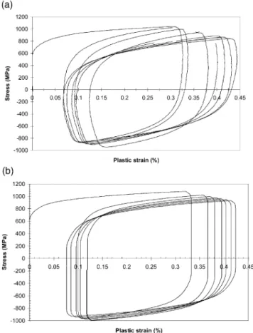
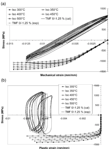
Evolutions of the hysteresis loops with increasing number of cycles is discussed in more detail for the OPC 0/#1.25% test. The first mechanical strain path from 0 to #1.25% during temperature change from 300°C to 500°C induces a large negative plastic strain as shown in Fig. 17. During this loading, a stress maximum is observed at a temperature of 450°C; superposition of the isothermal paths at 300°C, 350°C, 400°C, 450°C and 500°C show that the anisothermal stress strain path is the result of the successive isothermal points. At mechanical strain reversal, the stress–plastic strain plot is rounded and plastic strain continues to increase as a result of the non instantaneous plastic strain rate dropping to zero; when zero value is reached, the behaviour becomes lin-ear up to the point at which reversed plastic strain flow occurs. At this point, even if mechanical strain is nega-tive, the stresses are tensile and maximum tensile stress is obtained for the zero mechanical strain. It can be seen that even if the mechanical strain amplitude is high (1.25%) the anisothermal plastic strain amplitude is quite

Fig. 17. TMF, 300–500°C, "em=#0/#1.25% calculated and

experi-mental loops and Isothermal calculated 0/#1.25% initial load increase for 300°C, 350°C, 400°C, 450°C and 500°C. (a) Stress mechanical strain, (b) stress–plastic strain.

low. During the successive cycles, maximum and mini-mum stresses are shifted to higher stresses whereas the plastic strain loops move to higher negative plastic strains. Superposition of experimental curves show very good agreement between the model and test, and the model allows a good understanding of the experimental features during such complex anisothermal phenomena. Such a progressive shifting during the first cycles van-ishes when mechanical strain amplitude is increased, i.e. plastic strain amplitude is increased as shown in Fig. 18 where the first five stress strain loops for four different plastic strain amplitudes in the OPC conditions are plot-ted. Consequently, mean stress tends towards a stable non zero value faster if strain amplitude is high as observed experimentally and reported in Fig. 9. This phenomenon is the transposition of the isothermal mean stress relaxation during non symmetrical test conditions to the anisothermal fatigue regime, where mean stress relaxes towards a non-zero value depending only on the temperature range.

The relation between the mean stress and strain and temperature amplitudes was investigated in more detail with the model. Fig. 19 reports the calculated mean

Fig. 18. Calculated TMF 300–500°C, OPC cycles for four different mechanical strain amplitudes.

Fig. 19. Calculated mean stress evolution versus number of cycles during TMF cycling. Temperature amplitude 300–500°C and various IP, OP and OPC mechanical strain amplitudes.

stresses for the TMF cycling 300–500°C and strain amplitudes corresponding to the experimental test pro-gram. Model response is coherent with the experimental ones (Fig. 9) and all OP and OPC tests give a tensile mean stress of 230 MPa (respectively #230 MPa for IP). Moreover it was found that the mean stress is only related to the temperature range as shown in Fig. 20 for simulated TMF temperature ranges of 300–400°C, 400– 500°C and 300–500°C whatever the strain amplitude; respective levels are 91 MPa, 136 MPa and 230 MPa.

In order to confirm model formulation the first and 10th loops of the IP test of mechanical strain amplitudes of 1.4%, 2.0% and 2.5% are plotted in Fig. 21(a) and are compared to experimental response Fig. 21(b). Even if general features are well reproduced, two differences are nevertheless noticeable: first, the evolution between the first and 10th loop is more pronounced in the experi-mental plots, and secondly there is a small discrepancy in the increasing part of the loops where the model pre-dicts a stress maximum for lower strain values than the experimental results. But this may be related to the identification procedure where isothermal strain

ampli-Fig. 20. Calculated mean stress evolution versus number of cycles during TMF cycling. Temperature amplitudes 300–400°C; 300–500°C, 400–500°C and mechanical strain amplitudes IP and OP ±0.7% and OPC 0/#1.25%.

Fig. 21. IP 300–500°C TMF cycles for three different mechanical strain amplitudes. (a) Calculated, (b) experimental.

tudes taken into account are lower than those obtained in these TMF tests simulations.

Semi-stress amplitude ("s/2) evolution was calcu-lated over 500 cycles and is plotted in Fig. 22 for differ-ent anisothermal cycles. It can be seen that martensitic steels show cyclic softening in TMF conditions as observed in the isothermal fatigue conditions; softening

Fig. 22. Semi-stress amplitude for different TMF cycles versus (a) number of cycles and (b) cumulated plastic strain.

is rapid in the first stage and then flattens out. When plotting against the number of cycles [Fig. 22(a)], the exponential and the linear softening seem higher when the cyclic strain amplitude is higher, and for the same strain amplitude ("em=1.4%) softening is greater in IP

conditions than in OP or OPC conditions. This apparent discrepancy in linear softening disappears when the model internal variable “p” corresponding to the cumu-lated plastic strain is used as shown in Fig. 22(b), where it can be seen that linear softening phenomena is not strain amplitude dependant. It may be concluded that comparisons between different test conditions are more accurate if they are performed with respect to model variables instead of test parameters.

5. Conclusions

Two martensitic steels commonly used in the forging industry have been investigated in isothermal fatigue, especially with respect to their cyclic softening behav-iour which has been found to be influenced by tempera-ture, strain amplitude, strain rate and initial hardness. A TMF test facility was developed and used to evaluate the anisothermal cyclic behaviour of such steels in IP,

OP, and OPC fatigue conditions in the 300–500°C range where the steel undergoes no structural change.

An anisothermal elasto-viscoplastic constitutive model was formulated in the frame of the theory of irre-versible processes on the basis of the experimental fea-tures observed in isothermal fatigue. It takes into account kinematic hardening, strain rate and strain memory effects, and uses two back stresses to describe the non saturating softening of such steels. It was found relevant to describe the results of the anisothermal tests.

The following experimental and/or model simulation results have been found important:

1. During anisothermal fatigue, a mean stress is gener-ated which is tensile in OP conditions and compress-ive in IP conditions. Mean stress is independent of the mechanical strain amplitude for a fixed tempera-ture range, but changes if the temperatempera-ture range used for TMF tests changes. If the TMF test is performed in non symmetrical mechanical strain conditions, like the OPC conditions representative of forging tools, there is a progressive shifting of the loops towards a level where the mean stress no longer undergoes any changes; this phenomenon is the transposition to thermo mechanical fatigue of the “mean stress relax-ation” phenomenon well known under isothermal fatigue conditions.

2. Analysis of cyclic softening (i.e. semi-stress amplitude) against model internal variable “p” corre-sponding to the cumulated plastic strain is more accurate than the classical analysis against the number of cycles. It shows in particular that the linear soften-ing is an intrinsic feature of the material for a given temperature in isothermal fatigue or temperature range in TMF. It is independent of numerous test parameters like strain rate, strain amplitude, IP or OP cycling.

Acknowledgements

The authors gratefully acknowledge Olivier Brucelle for his contribution to anisothermal testing.

References

[1] Maiya PS, Majumdar S. Elevated temperature low cycle fatigue behaviour of differents heats of type 304 stainless steel. Metallur-gical Transactions 1977;8A:1651–60.

[2] Challenger KD, Moteff D. A correlation between strain hardening parameters and dislocation substructure in austenitic stainless steels. Scripta Metallurgica 1972;6:155–60.

[3] Kanazawa K, Yoshida S. Effect of temperature and strain rate on the high temperature low cycle fatigue behaviour of austenitic stainless steel. In: Proceedings of the International Conference on Creep and Fatigue in Elevated Temperature Applications, Lon-don, 1974. p. 226.1–226.10.

[4] Feltner CE, Laird C. Factors influencing the dislocations struc-tures in fatigued metals. Transactions of the Metallurgical Society of AIME 1968;242:1253–7.

[5] Mughrabi H, Microstructural aspects of fatigue, Dislocations et de´formation plastique, Ecole d’e´te´ d’Yravals, september 1979, edited by Les Editions de Physique, 1980. p. 363–73.

[6] Hu Z, Xiao J. Cyclic softening characteristics and mechanism of hot work die steels during low cycle fatigue. In: Fatigue 90, Proceedings of the 4th International Conference on Fatigue and Fatigue Thresholds, Honolulu, 1990. p. 469–74.

[7] Kanazawa K, Yamaguchi K, Kobayashi K. The temperature dependence of low cycle fatigue behaviour of martensitic stain-less steels. Materials Science and Engineering 1979;40:89–96. [8] Vogt JB, Degallaix G, Foct J. Cyclic mechanical behaviour and

microstructure of a 12Cr–Mo–V martensitic stainless steel. Fatigue and Fracture of Engineering Materials and Structures 1988;11:435–46.

[9] Vogt JB, Argillier S, Leon J, Massoud JP, Prunier V. Mech-anisms of cyclic plasticity of a ferrite–bainite 21

4Cr1Mo steel after

long-term service at high temperature. ISIJ International 1999;39:1198–203.

[10] Chai H, Fan Q. fatigue softening mechanism of low carbon tem-pered martensite. In: Fatigue 93, Proceedings of the 5th Inter-national Conference on Fatigue and Fatigue Thresholds, Mon-treal, 1993. p. 195–200.

[11] Wang ZG, Rahka K, Nenonen P, Laird C. Changes in mor-phology and composition of carbides during cyclic deformation ar room and elevated temperature and their effect on mechanical properties of Cr–Mo–V steel. Acta Metallurgica 1985;33:2129– 41.

[12] Estrin Y. A versatile unified constitutive model based on dislo-cation density evolution. High Temperature Constitutive Mode-ling—Theory and Application 1991;MD-Vol.26/AMD-Vol. 121:65–83.

[13] Miller AK. The MATMOD equation, unified constitutive equa-tions for creep and plasticity. London: Elsevier Applied Science, 1987.

[14] Chaboche JL. Constitutive equations for cyclic plasticity and cyc-lic viscoplasticity. International Journal of Plasticity 1989;5:247–302.

[15] Krempl E, McMahon JJ, Yao D. Viscoplacity based overstress with a differential growth law for the equilibrium stress. In: 2nd Symp. on Non Linear Constitutive Relations for High Tempera-ture Applications, NASA, Cleveland, OH. Mechanics of Materials 1986;5:35–48.

[16] Bodner SR. A review of an unified elastic-viscoplastic theory, unified constitutive equations for creep and plasticity. London: Elsevier Applied Science, 1987.

[17] Arnold SM, Saleeb. On the thermodynamic framework of gen-eralized coupled thermoelastic-viscoplastic damage model. Inter-national Journal of Plasticity 1994;10:263–78.

[18] Bernhart G, Moulinier G, Brucelle O, Delagnes D. High tempera-ture low cycle fatigue behaviour of a martensitic forging tool steel. International Journal of Fatigue 1999;21(2):179–86. [19] Delagnes D. Isothermal fatigue behaviour and lifetime of a 5%Cr

hot work tool steel around the LCF-HCF transition. PhD thesis, ENSMP, 1998.

[20] Joarder A, Cheruvu NS, Sarma DS. Influence of high temperature low cycle fatigue deformation on the microstructure of a CrMoV rotor steel subjected to long-term service exposure at 425°C and retempering at 677°C. Materials Characterisation 1992;28(4):121–31. [21] Zhang Z, Delagnes D, Bernhart G. Stress–strain behaviour of tool steels under thermo-mechanical loadings: experiment and model-ling. In: Proceedings of the 5th International tooling Conference, Leoben, 1999. p. 205–13.

l’en-dommagement en fatigue thermome´canique d’un acier a` outil (55NCDV7). Rapport de DEA, INP Toulouse, juin 1997. [23] Castelli MG, Ellis JR. Improved techniques for

thermomechan-ical testing in support of deformation modeling. ASTM STP 1993;1186:195–211.

[24] Sehitoglu H. Thermomechanical fatigue life prediction methods. ASTM STP 1992;1122:47–76.

[25] Zauter R, Petry F, Christ HJ, Mugrabi H. Thermomechanical fatigue of the austenitic stainless steel AISI 304L. ASTM STP 1993;1186:70–90.

[26] Kleinpass B, Lang KHK, Lo¨he D, Macherauch E. Thermal-mech-anical fatigue behaviour of NiCr22Co12Mo9. In: Bresser J, remay L, editors. Fatigue under thermal and mechanical loadings, 1996. p. 327–37.

[27] Germain P. Cours de me´canique de milieux continus. tome 1 Paris: Masson, 1997.

[28] Lemaitre J, Chaboche JL. Mechanics of solids. Cambridge: Cam-bridge University Press, 1990.

[29] Burlet H, Cailletaud G. Numerical techniques for cyclic plasticity at variable temperature. Eng Comput 1986;3(June):143–53. [30] Armstrong PJ, Frederick CO. A mathematical representation of

the multiaxial baushinger effect. GEGB Report RD/B/N 731. [31] Cailletaud G. Mode´lisation me´canique d’instabilite´s

microstruc-turales en viscoplasticite´ cyclique a` tempe´rature variable. PhD thesis, Universite´ Pierre et Marie Curie, 1979.

[32] Ohno N. A constitutive model of cyclic plasticity with non-hard-ening strain region. Journal of Applied Mechanics 1982;49:721. [33] Bernhart G, Zhang Z, Choi BG, Delagnes D. Single specimen methodology for elasto-visco-plastic fatigue model identification of martensitic steels. Euromat 2000 November:1077–82.