3D h-φ finite element formulation for the computation of a linear transverse flux
actuator
G. Deli´ege1, F. Henrotte1, H. VandeSande1, and K. Hameyer1
1Katholieke Universiteit Leuven
Dept. ESAT, Div. ELECTA
Kasteelpark Arenberg 10, B-3000 Leuven, Belgium e-mail: [email protected]
Abstract – A finite element analysis of a permanent magnet transverse flux linear actuator is presented. In this applica-tion where we need as well a small model (for optimisaapplica-tion purposes) as a high accuracy on the computed force, we pro-pose to combine several models with different levels of size and complexity, in order to progressively elaborate an accurate, but nevertheless tractable, model of the system.
1. Introduction
One of the typical outcomes of the numerical modeling of the dynamics of actuators is the estimation of the magnetic force exerted on moving parts. In the conception and the design of such devices, the geometry of the magnetic cores (and consequently of the airgap) is a fundamental issue. Op-timizing the geometry so as to match technical constraints requires numerous numerical computations of the system, which makes it highly desirable to dispose of a numerical model of small size. On the other hand, the exerted force depends on the distribution of the magnetic field around the moving part. It has always a 3D component, of which the relative importance depends on the geometry as well. The aim of this paper is to design a finite element model of a linear transverse flux actuator, which allows the computa-tion of the force with a given accuracy while minimizing the number of unknowns. The geometry and the main charac-teristics of the actuator are described. A 2D model and a simplified 3D model limited to a region around the mover are presented. A dual approach in both scalar potential and vector potential formulations is proposed. Two methods to compute the magnetic force on the mover are presented.
2. Description of the motor
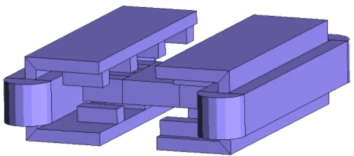
The permanent magnet transverse flux linear actuator under consideration aims at fast and accurate positioning. It has been described in previous papers [1][2]. The actuator con-sists of two independent motors facing each other (Fig. 1). The stators can be seen as long C-cores with toothed lower and upper plates. A coil is wound around each vertical core. The teeth of the two stators are shifted in space by a quarter of a pole pitch, so that the reluctance forces in the direc-tion of the movement, i.e. theX-axis, cancel each other out
[1][2]. The movers are made of blocks of iron and of blocks of high energy magnets magnetized in the X direction
al-ternately. A block of non-magnetic material is sandwiched between the movers in order to avoid flux passing from one mover to the other. The movers are therefore mechanically
Fig. 1. Geometry of the overall transverse flux linear actuator
connected but magnetically independent, and only one mo-tor needs to be modeled (Fig. 2). The magnet and iron blocks forming the mover have the same dimensions as the stator teeth in the X and Z directions. The pole pitch is
equal to four times the block length. The position of the mover is measured with respect to a reference position for which the first block of the mover is aligned with a stator tooth.
coil mover
stator
Fig. 2. Full 3D finite element model of the actuator
3. Finite element models
In this application where we need as well a small model (for optimisation purposes) as a high accuracy on the computed force, we propose to combine several models with different levels of size and complexity, in order to progressively
elab-orate an accurate, but nevertheless tractable, model of the system.
A. Airgap centered 3D model
When dealing with 3D models, it is important to use un-knowns sparingly. As the accuracy of the computed force depends mainly on the accuracy of the computed magnetic field in the airgap around the mover, we can advantageously leave the vertical core and the coil outside the model. There-fore, we have defined an airgap-centered 3D model, which focuses on the airgap field and devote a maximum of the available unknowns to the description of the field around the mover (Fig. 3). The airgap centered 3D model is connected
φ= 0 φ= I
(a) (b)
Fig. 3. (a) full 3D model and (b) focused 3D model of the actuator
to a simple magnetic circuit that accounts for the vertical core and the coil, in order to get in total a complete rigorous model of the system.
B. 2D model
The three-dimensional effects occurring around the mover cannot be taken into account by a two-dimensional model. However, the 2D approximation has definite advantages if compared to a full 3D approach: the geometry and the con-trol of the quality of the mesh are easier and faster; and the computation time is significantly lower. Therefore, the de-sign of a 2D model is generally a preliminary step which allows the designer to perform many computations to deter-mine the overall behaviour of the system, and to investigate the influence of the parameters, at a reduced computation cost. The 2D model is a slice of the motor in the X − Y
plane (Fig. 4). Two regions are added, above and under the stator teeth, to represent the part of the stator around which the coil is wounded. The problem is solved with both scalar potential and vector potential formulations as explained in the following section.
4. Finite element dual formulations
In this application, dual analysis is used to determine which refinement is necessary in the airgap to have the force on the mover computed with a given accuracy. This question can be answered satisfactorily in the context of a 2D analysis, because one may assume that the smallness of the charac-teristic mesh size needed to obtain a given accuracy will not depend crucially on the 3D effect. The costly dual analysis is therefore carried over with the simplified 2D model, in order to find out how fine the mesh in the airgap must be toΓU
ΓD
ΓL ΓR
Fig. 4. 2D finite element model
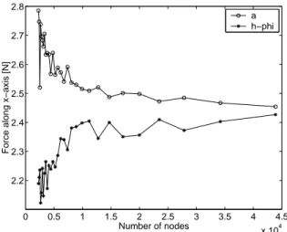
reach the desired accuracy and how coarser it can be at other places. The convergence of the force computed by the 2D dual formulations as a function of the total number of nodes of the mesh, is shown on Fig. 5. The values obtained with the dual approach give a valuable control on the accuracy. On basis of this curve, a relation can be found between the characteristic length of the elements of the mesh and the ac-curacy of the global quantities (force, energy). This relation helps designing the 3D model, by giving an approximation of the size and the distribution of the elements in the 3D mesh in order to reach a given accuracy. To illustrate the relative computation cost of the models, a 3D mesh of more than 500000 nodes is necessary to obtain the same accuracy as a 2D mesh of 20000 nodes. 0 0.5 1 1.5 2 2.5 3 3.5 4 4.5 x 10⁴ 2.2 2.3 2.4 2.5 2.6 2.7 2.8 Number of nodes
Force along x−axis [N]
a h−phi
Fig. 5. Convergence of the force computed in 2D with the a and
h− φ formulations ; flux ϕ= 0.002 Wb
The problem is magnetostatic and the Maxwell equa-tions (1-2) must be solved.
div b = 0 (1)
curl h = j (2)
A. Scalar potential formulation
The magnetic field h is decomposed into the sum of the gra-dient of the scalar magnetic potentialφ, and the source field
hs which must verifycurl hs = j, so that equation (2) is
automatically fulfilled.
h= hs− grad φ (3)
The constitutive law is
b = µ0(h + m) (4) m = 0 in air m(b) or m(h) in iron hc in permanent magnets (5)
where hcis a constant depending on the type of permanent
magnet. Replacing (3) in (4), and then in (1), we obtain
div(µ0(hs− grad φ + m)) = 0 (6)
of which the weak form is
Z Ω grad φ0 · (µ0(hs− grad φ + m)) dΩ − Z ΓL∪ΓR φ0 b· n dΓ = 0 , ∀φ0 ∈ Fh0(Ω) (7) with Fh0(Ω) = {φ ∈ L 2(Ω); grad φ ∈ L2(Ω), φ| ΓU∪ΓD = 0}. (8)
B. Vector potential formulation
The magnetic induction is expressed as b= curl a, in order
to fulfill (1). Equation (2) expressed in terms of the vector potential a becomes:
curl( 1 µ0
curl a − m) = j (9)
The weak form is
Z Ω curl a0 · ( 1 µ0 curl a − m) dΩ − Z ΓU∪ΓD (a0 ∧ h) · n dΓ = 0 , ∀a0 ∈ Fh1(Ω)(10) with Fh1(Ω) = {a ∈ L 2(Ω); curl a ∈ L2(Ω), n∧a| ΓL∪ΓR= 0}. (11) C. Boundary conditions
The boundary conditions for the 2D model (Fig. 4) are set according to Table I-II.
5. Force computation
A. Direct differentiation of energy and coenergy
An accurate computation of the force profile is one of the goals of this finite element analysis. The calculation of elec-tromagnetic forces by direct differentiation of the magnetic energy or coenergy is simple, easy to understand and per-fectly rigorous; but it is generally disregarded because it
TABLE I BOUNDARY CONDITIONS FOR THEh
− φFORMULATION FixI : ΓU : φ= I ΓD: φ= 0 ΓL∪ ΓR: b· n = 0 Fixϕ : ΓU : − R ΓUµ0(hs− grad φ + m) · n dΓ = ϕ ΓD: φ= 0 ΓL∪ ΓR: b· n = 0 TABLE II
BOUNDARY CONDITIONS FOR THEaFORMULATION
FixI: ΓU∪ ΓD: h∧ n = 0 ΓL: aZ= 0 ΓR: R ΓR( 1 µ0curl a − m) · n dΓ = I Fixϕ: ΓU∪ ΓD: h∧ n = 0 ΓL: aZ= 0 ΓR: aZ= ϕ
requires to solve several times the system. However, this drawback vanishes if one is interested in the force, not at one particular position, but over a range of positions. The total magnetic coenergyΦ and magnetic energy Ψ of the
system are given by
Φ(h) = Z Ω 1 2µ0(h + m) 2 dΩ (12) Ψ(b) = Z Ω 1 2 µ0 b· b − m · b dΩ (13)
Making use of (4), one checks easily that expressions (12) and (13) verify the relation
Ψ(h) + Φ(b) = Z
Ω
b· h dΩ . (14)
In soft magnetic materials, hc vanishes and we obtain the
classical expressions of energy and coenergy. In permanent magnets, we have a situation represented in Fig. 6 for a given working point(b, h) such that b · h and Φ are negative.
No-tice that in that case,Φ and Ψ are not equivalent.
The coenergyΦ(h) is computed when the scalar
poten-tial formulation is used, whereas the energyΨ(b) is
com-puted when the vector potential formulation is used. Since the problem is solved for a set of successive positions of the mover, we can easily compute the value of the component of the force in the direction of motion at any pointxi, with
a second order approximation of the derivative of the coen-ergy or the encoen-ergy:
Fx(xi) = Ψ(xi+1) − Ψ(xi−1) xi+1− xi−1 = −Φ(xi+1) − Φ(xi−1) xi+1− xi−1 (15)
B H br= µ0hc −hc (h, b) Φ −Ψ
Fig. 6. Energy and coenergy in the magnet
B. Eggshell method
On the other hand, if one is interested in the transient anal-ysis of the actuator, a method that gives directly the force at each position is needed. There are two possibilities, the virtual work principle and the Maxwell stress tensor.
The virtual work method is fairly general but not easy to understand nor to implement. Moreover, the generality of this costly method is not fully exploited in this particu-lar case where, instead of the local values at nodes of the magnetic force, the resultant force exerted on a rigid body is sought after. It is therefore worth finding a more dedicated and efficient method. The technique we have adopted, i.e. the eggshell method [8], stems from the application of the Maxwell stress tensor. The latter is precisely valid for the computation of the magnetic forces exerted on rigid bodies placed in air. A direct application of the Maxwell stress ten-sor requires however to integrate over a surface an expres-sion of which the computation requires information coming from outside the surface (i.e. the normal gradient of the po-tential). This makes it necessary to find out, for each inte-gration point in the surface, the finite element to which it belongs. The eggshell method is a particular application of the Maxwell stress tensor that avoids this disadvantage. It consists in averaging the Maxwell stress tensor over a con-tinuous class of concentric closed surfaces, which fill up an eggshell shaped regionΩBplaced around the moving body
(Fig. 7). Arkkio’s famous formula for torque computation in electrical machines [4] results from the application of the same principle in the airgap of an electrical machine, assum-ing a rigid body rotation of the rotor.
The parallelepipedic eggshell shown in Fig. 7 can in that way be considered as filled up by a class of parallelepipedic surfaces enclosed inside each other. The normal to all those surfaces make up a unit vector field n that is uniform over each of the six walls of the eggshell. It can usually be de-fined analytically. For rigid body translations, the eggshell
ΩB
Fig. 7. Eggshell region ΩBenclosing a layer of air and the mover (grey volume)
method formulae are:
F= Z ΩB µ0 δ (h (h · n) − 1 2n(h · h)) dΩB (16) F= Z ΩB 1 µ0δ (b (b · n) −1 2n(b · b)) dΩB (17)
whereδ is the thickness of the eggshell.
0 0.2 0.4 0.6 0.8 1 −5 −4 −3 −2 −1 0 1 2 3 4 5
Mover position [pole pitches]
Force along x−axis [N]
2D, eggshell 2D, coenergy 3D, eggshell 3D, coenergy
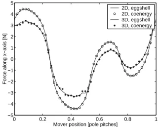
Fig. 8. Comparison of the forces computed with the eggshell method and the differentiation of coenergy, in 2D and 3D (h − φ)
Fig. 8 shows a comparison between the two methods used for force computation. They give similar results, as well in 2D as in 3D, but the method based on the direct dif-ferentiation of energy suffers from the loss of accuracy due to the numerical differentiation.
In total, the eggshell method is more interesting because it requires only the integration over a smaller volume (ΩB
instead of the complete domain) and all the needed informa-tion is contained in that small volume. We have also found it to be more accurate in the 3D case.
6. Results
A first set of calculations has been done with the 3D and the 2D models, using the h− φ formulation. The 2D and
mover displaces over one pole pitch and for each position, the coil current takes the five values−200 A, −100 A, 0 A, 100 A and 200 A.
0 0.2 0.4 0.6 0.8 1
0.06 0.07 0.08
Mover position [pole pitches]
Coenergy of the system [J] −200 A −100 A 0 A 100 A 200 A
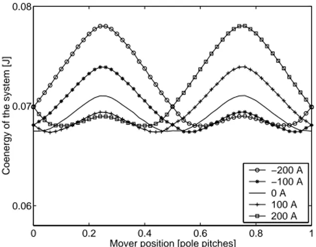
Fig. 9. 3D (h − φ): coenergy of the system as the coil current ranges from −200 A to 200 A
0 0.2 0.4 0.6 0.8 1
0.06 0.07 0.08
Mover position [pole pitches]
Coenergy of the system [J]
−200 A −100 A 0 A 100 A 200 A
Fig. 10. 2D (h − φ): coenergy of the system as the coil current ranges from −200 A to 200 A
One sees in general that the 3D effect influences sensibly the energy and coenergy of the system (Fig. 9-10), as well as the developed force (Fig. 11-12) but that the 2D model captures the most important features of the behaviour of the device. The 3D effect of the force is not a simple multipli-cation factor but it depends on the position of the mover. It can be estimated from Fig. 8.
The shape of the curves, the relative influence of the coil currents, are all qualitatively well described by the 2D model, at a much lower computational cost and with a much better continuity. They give a justification that one can pur-sue as far as possible the geometrical optimisation with the 2D model. It suggests indeed that the optimum configura-tion found by the 2D analysis will not be very different from the real optimum. The slight irregularities of the curves rep-resenting the force profiles computed in 3D (Fig. 11) show that the 3D mesh is too coarse, even if the number of nodes is ten times greater than in the 2D mesh and despite the fact
0 0.2 0.4 0.6 0.8 1 −5 −4 −3 −2 −1 0 1 2 3 4 5
Mover position [pole pitches]
Force along x−axis [N]
−200 A −100 A 0 A 100 A 200 A
Fig. 11. 3D (h − φ): force along X computed with the eggshell method, as the coil current ranges from −200 A to 200 A
0 0.2 0.4 0.6 0.8 1 −5 −4 −3 −2 −1 0 1 2 3 4 5
Mover position [pole pitches]
Force along x−axis [N]
−200 A −100 A 0 A 100 A 200 A
Fig. 12. 2D (h − φ): force along X computed with the eggshell method, as the coil current ranges from −200 A to 200 A
that, due to the presence of the eggshell, there are several layers of elements in the airgap. This accuracy problem is obviously attributable to a lack of accuracy of the solution it-self, and not to the method used to compute the force, since the results obtained by the differentiation of the coenergy and the eggshell method confirm each other (Fig. 8). The oscillations of the curves in Fig. 8 come from the fact that the number of layers of elements in the eggshell increases discontinuously with the total number of elements.
7. Conclusion
A linear transverse flux actuator has been described. A two-dimensional and a simplified three-two-dimensional finite ele-ment model of the machine have been proposed in order to reduce the computation time, with a view to the optimisation of the force on the mover. The dual h− φ scalar potential
and a vector potential formulations in presence of perma-nent magnet materials have been reminded. Two methods to compute the force have been described, and their respective advantages have been pointed out. The finite element
mod-els have then been used to compute the force acting on the mover, as a function of its position and the coil current. It has been shown that the 2D analysis is unable to describe all the 3D effects, and to accurately evaluate the amplitude of the force and of the energy or coenergy of the system. How-ever, it can describe the important features of the behaviour of the device, and give an idea of the sensitivity of the global quantities to a variation of parameters, at a much lower com-putation cost. In addition, the 2D formulations are in some cases easier to implement: the vector potential formulation, for instance, does not require to build a spanning-tree for gauging. Therefore, if it cannot substitute for a 3D analysis, it nevertheless constitutes a valuable preliminary and com-plementary step.
Acknowledgement
The authors are grateful to the Belgian ”Fonds voor Weten-schappelijk Onderzoek Vlaanderen” for its financial support of this work and the Belgian Ministry of Scientific Research for granting the IUAP No. P4/20 on Coupled Problems in Electromagnetic Systems.
References
[1] H. Vande Sande, G. Deli´ege, K. Hameyer, H. Van Reusel, W. Aerts, and H. De Coninck, “Design of a linear transverse flux actuator for fast positioning”, Proceedings of the XII-Ith Conference on the Computation of Electromagnetic Fields (COMPUMAG2001) (Evian, France), July 2001, pp. 54–55.
[2] G. Deli´ege, H. Vande Sande, K. Hameyer, and W. Aerts, “3D finite element computation of a linear transverse flux actua-tor”, Proceedings of the International Conference on Power Electronics, Machines and Drives (PEMD2002) (Bath, UK), April 2002, pp. 315-319.
[3] H. Weh and J. Jiang, “Berechnungsgrundlagen f¨ur transver-salflußmaschinen”, Archiv f¨ur Elektrotechnik, Vol. 71. [4] Arkkio, “Analysis of induction motors based on the
numeri-cal solution of the magnetic field and circuit equations”, Acta
Polytechnica Scandinavica, page 56, 1987.
[5] R. Blissenbach, U. Sch¨afer, W. Hackmann, and G. Hen-neberger, “Development of a transverse flux traction motor in a direct drive system”, Proceedings of the International Con-ference on Electrical Machines (ICEM00) (Helsinki, Finland), August 2000.
[6] E.R. Laithwaite and H.R. Bolton, Linear motors with
trans-verse flux, Proceedings IEE, Vol. 118, no. 12.
[7] J.P. Webb and B. Forghani, “A single scalar potential formula-tion for 3D magnetostatics using edge elements”, IEEE
Trans-actions on Magnetics, Vol. 25, no. 11, pp. 4126-4128, 1989.
[8] F. Henrotte, G. Deli´ege, and K. Hameyer, “The eggshell method for the computation of electromagnetic forces on rigid bodies in 2D and 3D”, Proceedings of IEEE
Confer-ence on Electromagnetic Field Computation (CEFC2002)
(Pe-rugia,Italy), June 16-19 2002.
[9] P. Dular, C. Geuzaine, A. Genon and W. Legros, “An evolutive software environment for teaching finite element methods in electromagnetism”, IEEE Transactions on Magnetics, Vol. 35, no. 3, pp. 1682-1685, 1999.