arXiv:1010.6195v1 [astro-ph.CO] 29 Oct 2010
Astronomy & Astrophysicsmanuscript no. XMM˙LSS˙28102010 c ESO 2010
November 1, 2010
The XMM-LSS survey: optical assessment and properties of
different X-ray selected cluster classes
⋆
C. Adami
1, A. Mazure
1, M. Pierre
2, P.G. Sprimont
3, C. Libbrecht
2, F. Pacaud
2,8, N. Clerc
2, T. Sadibekova
3, J.
Surdej
3, B. Altieri
4, P.A. Duc
2, G. Galaz
7, A. Gueguen
2, L. Guennou
1, G. Hertling
7, O. Ilbert
1, J.P. LeF`evre
14, H.
Quintana
7, I. Valtchanov
4, J.P. Willis
9, M. Akiyama
12, H. Aussel
2, L. Chiappetti
10, A. Detal
3, B. Garilli
10, V. LeBrun
1, O. LeF`evre
1, D. Maccagni
10, J.B.
Melin
13, T.J. Ponman
11, D. Ricci
3, and L. Tresse
11 LAM, OAMP, Pˆole de l’Etoile Site Chˆateau-Gombert 38, Rue Fr´edr´eric Juliot-Curie, 13388 Marseille, Cedex 13, France 2 Laboratoire AIM, CEA/DSM/IRFU/Sap, CEA-Saclay, F-91191 Gif-sur-Yvette Cedex, France
3 Institut d’Astrophysique et de G´eophysique, Universit´e de Li`ege, All´ee du 6 Aoˆut, 17, B5C, 4000 Sart Tilman, Belgium 4 ESA, Villafranca del Castillo, Spain
5 UPMC Universit´e Paris 06, UMR 7095, Institut d’Astrophysique de Paris, F-75014, Paris, France 6 CNRS, UMR 7095, Institut d’Astrophysique de Paris, F-75014, Paris, France
7 Departamento de Astronom´ıa y Astrof´ısica, Pontificia Universidad Cat´olica de Chile, Casilla 306, Santiago 22, Chile 8 Argelander-Institut f¨ur Astronomie, University of Bonn, Auf dem H¨ugel 71, 53121 Bonn, Germany
9 Department of Physics and Astronomy, University of Victoria, Elliot Building, 3800 Finnerty Road, Victoria, V8V 1A1, BC, Canada 10 INAF-IASF Milano, via Bassini 15, I-20133 Milano, Italy
11 School of Physics and Astronomy, University of Birmingham, Edgbaston, Birmingham, B15 2TT, UK 12 Astronomical Institute, Tohoku University 6-3 Aramaki, Aoba-ku, Sendai, 980-8578, Japan
13 CEA/DSM/IRFU/SPP, CEA Saclay, F-91191 Gif-sur-Yvette, France. 14 CEA/DSM/IRFU/SEDI, CEA Saclay, F-91191 Gif-sur-Yvette, France Accepted . Received ; Draft printed: November 1, 2010
ABSTRACT
Context.XMM and Chandra opened a new area for the study of clusters of galaxies. Not only for cluster physics but also, for the detection of faint and distant clusters that were inaccessible with previous missions.
Aims. This article presents 66 spectroscopically confirmed clusters (0.05≤z≤1.5) within an area of 6 deg2 enclosed in the XMM-LSS survey. Almost two thirds have been confirmed with dedicated spectroscopy only and 10% have been confirmed with dedicated spectroscopy supplemented by literature redshifts.
Methods.Sub-samples, or classes, of extended-sources are defined in a two-dimensional X-ray parameter space allowing for various degrees of completeness and contamination. We describe the procedure developed to assess the reality of these cluster candidates using the CFHTLS photometric data and spectroscopic information from our own follow-up campaigns.
Results.Most of these objects are low mass clusters, hence constituting a still poorly studied population. In a second step, we quantify correlations between the optical properties such as richness or velocity dispersion and the cluster X-ray luminosities. We examine the relation of the clusters to the cosmic web. Finally, we review peculiar structures in the surveyed area like very distant clusters and fossil groups.
Key words.Surveys ; Galaxies: clusters: general; Cosmology: large-scale structure of Universe.
Send offprint requests to: C. Adami e-mail: [email protected]
⋆ Based on observations obtained with MegaPrime/MegaCam, a
joint project of CFHT and CEA/DAPNIA, at the Canada-France-Hawaii Telescope (CFHT) which is operated by the National Research Council (NRC) of Canada, the Institut National des Science de l’Univers of the Centre National de la Recherche Scientifique (CNRS)
of France, and the University of Hawaii. This work is based in part on data products produced at TERAPIX and the Canadian Astronomy Data Centre as part of the Canada-France-Hawaii Telescope Legacy Survey, a collaborative project of NRC and CNRS. This work is also based on observations collected at TNG (La Palma, Spain), Magellan (Chile), and at ESO Telescopes at the La Silla and
2 Adami et al.: Optical assessment and comparative study of the C1, C2, and C3 cluster classes
1. Introduction
With the quest for the characterisation of the Dark Energy properties and the upcoming increasingly large instruments (JWST, ALMA, LSST, EUCLID, etc. ...) the beginning of the 21st century is to be an exciting time for cosmology. In this respect, a new era was already open for X-ray astronomy by the XMM-Newton and Chandra observatories in 1999. The increasing amount of high quality multi-wavelength observations along with the concept of “multi-probe” approach is expected to provide strong constraints on the cosmological models. In this context, X-ray surveys have an important role to play, as it was already the case in the 80s and 90s (e.g. Romer et al. 1994, Castander et al. 1995, Collins et al. 1997, Henry et al. 1997, Bohringer et al. 1998, Ebeling et al. 1998, Jones et al. 1998, Rosati et al. 1998, Vikhlinin et al. 1998, De Grandi et al. 1999, Romer et al. 2000, and ref. therein). New cluster surveys are presently coming to birth (e.g. Romer et al. 2001, Pierre et al. 2004, Finoguenov et al 2007).
One of them, the XMM-LSS survey, covers 11 deg2 at a sensitivity of ∼ 10−14 erg/s/cm2 at 0.5-2keV for spatially-extended X-ray sources and is currently the largest contigu-ous deep XMM cluster survey. This sky region is covered by parallel surveys in multiple complementary wavebands rang-ing from radio to the γ-ray wavelengths (Pierre et al., 2004) and therefore constitutes a unique area for pioneering studies. It can for instance detect a Coma-like cluster at z∼2. A number of articles describing the properties of the XMM-LSS source population have been published by e.g. Pierre et al (2006) and Pacaud et al (2007) for clusters of galaxies and Gandhi et al (2006) for AGNs; the complete X-ray source catalog along with optical identifications for the first 5 deg2 of the survey was published by Pierre et al (2007).
One of the major goals of the XMM-LSS survey is to pro-vide samples of galaxy clusters with well defined selection cri-teria, in order to enable cosmological studies out to redshift
z ∼ 1.5. Indeed, monitoring selection effects is mandatory not
only to study the evolution of the cluster X-ray luminosity (i.e. mass) function or of the 3-D cluster distribution but also, as shown by Pacaud et al. (2007), to characterise the evolution of the cluster scaling laws such as the luminosity-temperature relation. We have put special emphasis on the X-ray selection criteria in the XMM-LSS survey. The procedure enables the construction of samples having various degrees of complete-ness and allows for given rates of contamination by non clus-ter sources. The subsequent optical spectroscopic observations constitute the ultimate assessment of the clusters, thus operates the purification of the samples.
In a first paper, Pacaud et al (2007) presented the Class One (C1) clusters pertaining to the first 5 deg2 of the survey (the ones with the highest apriori probability to be real clus-ters). The C1 selection yields a purely X-ray selected cluster sample with an extremely low contamination level and corre-sponds to rather high surface brightness objects. The present article summarises these former findings including now the Paranal Observatories under programmes ID 072.A-0312, 074.A-0476, 076.A-0509, 070.A-0283, 072.A-0104, and 074.A-0360.
clusters selected from less stringent X-ray criteria (C2 and C3) and including the contiguous Subaru Deep Survey (SXDS, e.g. Ueda et al. 2008). The C2 and C3 objects presented here come from an initial sample with a higher degree of contamination, but have all passed the final spectroscopic tests. Compared to the C1 clusters, they are fainter and correspond a-priori to less massive clusters or to groups at a redshift of ∼0.5: this is a population that is for the first time systematically unveiled by the XMM-LSS survey. A few massive very distant clusters are falling into this category too.
The present study is the first attempt to give a comprehen-sive census (X-ray and optical properties) of the low-mass clus-ter population within the 0 < z < 1 range. Search for correla-tions between optical and X-ray properties has already been a long story from, e.g, Smith et al. (1979) or Quintana & Melnick (1982). However, with more than 60 spectroscopically con-firmed clusters, the current sample constitutes, by far, the spec-troscopically confirmed cluster sample with the highest sur-face density ever published. The article is organised as follows. Next section describes the X-ray cluster selection. Section 3 presents the available optical photometric and spectroscopic data. Section 4 explains the adopted cluster validation proce-dure, the new X-ray luminosity computations, and presents the resulting catalog. Then, the global properties of each cluster class and category are examined in Section 5 and, subsequently, the properties of the cluster galaxy population in Section 6. Section 7 details the z=1.53 cluster and investigates possible peculiar structures in the survey. Finally Section 8 gathers the conclusions. The two appendixes discuss the accuracy of pho-tometric redshifts in the context of dense environments and lists additional redshift structures found in the course of the study.
Throughout the paper we assume H0 = 71 km s−1 Mpc−1, Ωm=0.27, and ΩΛ=0.73 (Dunkley et al 2009). All magnitudes
are in the AB system.
2. The initial cluster candidate selection
The clusters presented in this paper are for the great majority X-ray selected. The XMM-LSS pipeline (Pacaud et al 2006) provides for each detected source some 20 parameters (co-ordinates, count rate, etc..). Out of these, two are especially relevant for the characterisation of extended sources: the extent measurement (EXT) and the likelihood of extent (EXT LH). We recall (as defined by Pacaud et al 2006) that the ”extent” pa-rameter is the core radius of the beta-profile fit by the survey pipeline to each source, assuming a fixed beta of 2/3. The clus-ter selection basically operates in this two-dimensional space and has been extensively adjusted and tested using simulations of hundreds of XMM images. This allows the definition of three cluster samples.
– The C1 class is defined such that ∼ no point sources are misclassified as extended (i.e. less than 1% of the cluster candidates are point sources) and is described by EXT > 5′′,
EXT LH >33 plus an additional boundary on the detection likelihood, set to be greater than 32.
– The C2 class is limited by EXT > 5′′, EXT LH > 15 and
Adami et al.: Optical assessment and comparative study of the C1, C2, and C3 cluster classes 3
– The C3 clusters are faint objects and thus, have less-well characterized X-ray properties. They may be located at the very edge of the XMM field of view or suffer contamination by point sources. They therefore result from a subjective se-lection mostly based on a visual inspection of the X-ray and optical data; their selection function is up to now undefined. More details about the classification can be found in Pacaud et al (2006) and Pierre et al (2006).
In this paper, we have presented a large sample of X-ray clusters, including the 29 C1 confirmed clusters published by Pacaud et al. (2007). These C1 clusters were already unambigu-ously confirmed, but we take the occasion of this publication to reprocess the associated optical spectroscopic data follow-ing the standard method developed in the present paper. This will provide a unique homogeneous cluster sample. The clus-ters pertaining to this paper are, for most of them, located in the first 5 deg2of the XMM-LSS region, supplemented by the Subaru Deep Survey. The validated C1, C2, and C3 samples are presented in Tables 2, 3, and 4. In these Tables, XLSS catalog names refer to sources published in Pierre et al. (2007). XLSSU catalog names refer to sources whose fields were not yet considered in XLSS (for example flagged bad or in SXDS fields) and reobserved (or reprocessed later), or which were be-low the detection likelihood threshold in the input data set used as source for XLSS.
In the course of the data inspection, we have also identi-fied a few clusters using optically based criteria such as the red sequence or the gapper method. Our spectroscopic data set al-lowed us to confirm them as bona fide clusters, although these objects are not detected in the X-rays by the current version of the XMM-LSS pipeline or the association between X-ray de-tected sources and optical clusters is not straightforward. We thought of interest to publish these objects and they are listed in Tables 5 and B.1.
We now describe the involved optical data and the general identification processes.
3. The optical data
3.1. The optical spectroscopic data
We have been performing a dedicated spectroscopic follow-up of all C1 clusters and of a number of C2 and C3 clusters. These PI observations are listed in Table 1 and provide about 2000 redshifts to date. We supplemented this data set with the VVDS deep (e.g. LeF`evre et al. 2005: ∼11000 redshifts in 0.49 deg2) and ultradeep (LeF`evre et al. in preparation) data, and with a redshift compilation pertaining to the Subaru Deep Survey (Ueda et al 2008) included in the XMM-LSS area. Some 200 other redshifts were also available from NED for part of the area. We show in Fig. 1 the location of these different surveys, as well as the exposure time of the different XMM fields.
Individual redshift measurements of spectra resulting from the PI data were made following a procedure similar to that adopted by the VVDS survey. Each spectrum was indepen-dently measured by several people and the redshift subse-quently validated by a moderator. Quality flags were assigned
Fig. 1. Map showing the different involved surveys. The grey level disks are the 11’ central areas of the XMM pointings (ex-posure time depends on the greyness). Large squares show the spectroscopic VVDS-deep and Subaru Deep surveys, and the CFHTLS D1 field. C1, C2, and C3 clusters are also shown. Above a declination of -3.6deg, only g’,r’,z’ coverage is avail-able, hence no photometric redshifts are derived for this zone. Table 1. PI spectroscopic runs involved in the present paper.
Telescope Instrument Year Nights Run ID
Magellan LDSS2 2002 2 -Magellan LDSS2 2003 4 -NTT EMMI 2003 3 72.A-0312 NTT EMMI 2004 4 74.A-0476 NTT EMMI 2005 3 76.A-0509 TNG DOLORES 2007 4 AOT16/CAT 75 VLT FORS2 2002 3 70.A-0283 VLT FORS2 2003 4 72.A-0104 VLT FORS2 2004 4.5 74.A-0360
to each measurement following the VVDS rules: flag 0 indi-cates an inconclusive result, flag 1 means a probability of 50% that the assigned redshift is wrong, flag 2 means a probability of 25%, flag 3 means a probability of 5%, flag 4 means a prob-ability of 1%, and flag 9 means we have assigned a redshift with a single line using absent lines in order to limit the pos-sibilities. These percentage levels proved to be reliable in the VVDS survey (LeF`evre et al. 2005).
Our spectroscopic redshifts having quite heterogeneous ori-gins (different telescopes, instrumentations, and resolutions), it is therefore useful to compute the ability to measure a redshift and the achieved velocity resolution. In order to achieve such a goal, we chose to compare the PI data to the VVDS survey, which provides a well qualified set of data. Only 26 galaxies
4 Adami et al.: Optical assessment and comparative study of the C1, C2, and C3 cluster classes both measured by the VVDS and our dedicated follow-up have
a quality flag greater or equal than 2. For these objects, given the VVDS quality flags (6 flags 2, 6 flags 3, and 14 flags 4), we expect to have 3.2 wrong redshifts. We indeed find 3 red-shifts differing by more than 0.05 between the PI and VVDS data. VVDS spectroscopic redshifts are expected to have a typ-ical uncertainty of 280 km/s (from repeated VVDS redshift measurements, Le F`evre et al. 2005). Excluding all redshifts with differences greater than 0.02, we find a typical uncer-tainty between PI and VVDS redshifts of 340 km/s. Even with a comparison done on a rather limited size sample, the PI red-shifts appear thus reliable in the [0.,1.] redshift range and in the [18,23] I VVDS magnitude range.
Finally, it has to be mentioned that, for the spectroscopic sample, no completeness, neither spatial nor in luminosity, can be globally defined because of the various data origins.
3.2. The optical photometric data
Most of the XMM-LSS area is covered by the Canada-France-Hawaii Telescope Legacy Wide Survey (CFHTLS-Wide1). This survey, performed by means of the MegaCam camera, covers some 171 deg2in 4 independent patches with five filters (u∗, g′,r′,i′and z′). Resulting catalogs are 80% complete down to i′AB=24. The Wide survey encloses a sample of about 20×106 galaxies inside a volume size of ∼ 1 Gpc3, with a median red-shift of z∼ 0.92 (Coupon et al 2009). Northern of Dec= -3.6 deg, the CFHTLS data were complemented by PI MegaCam observations (3 deg2) performed in g’, r’, z’ at the same depth as the CFHTLS; they were reduced following the same proce-dure.
The optical images and catalogs were primarily used to check for the presence of galaxy concentrations coinciding with the extended X-ray emission. The CFHTLS data (only the T0004 release was available at the beginning of the present study) enabled the determination of photometric redshifts in the best fit template (Coupon et al. 2009). These photometric redshifts cover 35 deg2in the T0004 partially overlapping with the XMM-LSS area. They were computed using a template-fitting method, calibrated with public spectroscopic catalogs. The method includes correction of magnitude systematic off-sets. The achieved photometric redshift precision σz/(1+z) is
of the order of 0.04 with a catastrophic error percentage of less than 5% at i’≤23 (the magnitude limit we adopted for the pho-tometric redshifts).
4. ”Cluster candidate” validation process 4.1. General method
Extragalactic extended X-ray emission is the signature of a deep gravitational potential well. Apart from the hypotheti-cal ”dark clusters”, this potential well coincides with a galaxy over-density. The system (cluster or group) is therefore de-tectable using optical information only. In this article, we aim at assessing the presence of optical structures corresponding
1 http://terapix.iap.fr/cplt/T0006/T0006-doc.pdf
to the X-ray cluster candidates. Such systems are expected to manifest themselves as compact structures in redshift space (both spectroscopic and photometric ones) and as localized ex-cess in projected galaxy density maps.
To perform such an analysis, we make use of the two op-tical data sets mentioned above. The investigated lines of sight (centered on the X-ray emissions) were initially selected from the condition that at least two spectroscopic redshift measure-ments (whatever their values) are available within the X-ray isophotes. The subsequent conditions were more stringent de-pending on the cluster nature (see below).
The CFHTLS Wide survey and subsequent analyses (e.g. Coupon et al. 2009) provide us with galaxy positions as well as their apparent and absolute magnitudes, photometric redshifts and the corresponding ”galaxy types” T (from the spectral fit-ting performed during the photometric redshift computation). With the exception of the usual ”masking problems” due to bright stars or CCD defaults, photometric data are homoge-neous and allow us to define complete sub-samples in terms of spatial extension or in magnitudes. Limitations to these data are the redshift range within which photometric redshifts are reliable and the adopted magnitude limit. Here we restrict our-selves to 0.2 < z < 1.2 and i′ = 23 (see Coupon et al. 2009).
This limiting magnitude will affect partly the use of photomet-ric data to detect structures. Indeed, the characteristic magni-tude m* of the Schechter luminosity function is about i′ = 20
at z = 0.5 and i′= 22.5 at z = 1 leading to sampled luminosity function ranges of about m*+ 3 to m* + 0.5 at these respective redshifts. One drawback is therefore that for z > 0.5 the num-ber of galaxies actually belonging to a structure will be rapidly overcome by the background contamination (see e.g Table 1 of Adami et al 2005). One way to fight this contamination will be to use redshift slices defined on a photometric redshift basis (see Mazure et al. 2007) but the range covered in magnitude by structure members will remain limited.
In order not to bias the optical characterisation of the X-ray sources, the information concerning the C1, C2, C3 classifica-tion was used only at the very final stage.
4.2. Different analysis steps
The first step concerns the expected compactness in spectro-scopic redshift space. To reveal such compact associations, we used the already well tested and used ”gap method” (e.g. Biviano et al 1997, Rizzo et al 2004). It looks for significant gaps between successive galaxy velocities within the ordered redshift distribution obtained along a given line of sight. As in Adami et al (2005), we use a gap defined by g = 600 (1+z) km/s which was optimum for the considered redshift range. When the velocity difference between 2 successive galaxies is smaller than g, they are assigned to belong to a common structure, oth-erwise they are put in different groups.
Since the lines of sight most of the time sample redshifts up to at least z = 1, this first step of the analysis ends in gen-eral with sevgen-eral groups. Thus, with the mean redshift of every group, a cosmological distance was assigned, a physical region of 500 kpc (radius) defined and the galaxies within this radius
Adami et al.: Optical assessment and comparative study of the C1, C2, and C3 cluster classes 5 are selected as potential real cluster members. We choose this
size as being representative of clusters in terms of membership of galaxies w.r.t the field. Taking larger regions would decrease any real contrast, while taking smaller regions would decrease the number of true members. As a second step we then apply the usual ROSTAT tools (Beers et al. 1990) on individual red-shift groups to test for final membership and definition of the group properties (robust redshift locations and scales with their corresponding bootstrap errors).
As already mentioned, several groups are in general identi-fied along the lines of sight. Before comparing the galaxy distri-bution and the X-ray isophotes, we used then, when available, the CFHTLS photometric redshift information. As a third step, we selected galaxies in photometric redshift slices (of width: ±0.04 (1+z), see Coupon et al. 2009) around the mean red-shift of the considered group and produced iso-contours of nu-merical galaxy density (see Mazure et al 2007 for details and previous application). It is expected that the optical group phys-ically associated with the X-ray emission will show up with a clear density contrast located next to the position of the X-ray center. This is because the use of photometric redshift slices re-moves a large part of the fore and background contaminations. We also look, as another check, at the photometric redshift dis-tribution within various central regions compared to the one in the largest available region, conveniently renormalized and de-fined as the ”field”. Again, one expects a clear contrast at the redshift values given by the spectroscopy.
An illustration is given with the source XLSSC 013 in the XMM-LSS database. Three main groups were identified along the line of sight (z ∼ 0.2 with 9 redshifts, z∼ 0.3 with 26 red-shifts, z ∼ 0.6 with 5 redshifts). Consecutive examination of both the photometric redshift distribution and the numerical density histograms gives strong evidence for the z∼0.3 group to be chosen (see Figs. 2 and 3).
However, as mentioned above, photometric redshift data were not always available and spectroscopic data could be very sparse (our velocity dispersion measurements are then subject to very complex selection functions in the target selection when measuring and collecting galaxy redshifts). The final selection is then done by a visual inspection of X-ray and optical maps taking into account all the informations available. Fig. 3 shows the group at z = 0.3 chosen for XLSSC 013. As an extreme contrary case, we show in Fig. 4 XLSSC 035 for which only a few redshifts were available. The fact that a giant galaxy at z = 0.069 lies at the center finally pleads in favor of that redshift (Fig. 4) in the present paper. We note however that a z∼0.17 galaxy layer is also detected along this line of sight and we could deal with a superposition effect.
4.3. Results
We examined 34 C1 candidate X-ray sources. Identification fails for only two lines of sight mainly because very few red-shifts were available in the X-ray region and/or no photometric redshifts. All identified sources were classied as galaxy ters; this means that at least 95% of the C1 objects are real clus-ters (when obvious nearby galaxies - which show also a diffuse
36.8 36.82 36.84 36.86 36.88 36.9 -4.6 -4.56 -4.54 -4.52 -4.5 36.8 36.82 36.84 36.86 36.88 36.9 -4.58 -4.56 -4.54 -4.52 36.8 36.82 36.84 36.86 36.88 36.9 -4.58 -4.56 -4.54 -4.52 -4.48
Fig. 2. Isodensity maps of the numerical density of galaxies within photometric slices of width ± 0.04 (1+z) around the group redshifts. From top to bottom: z ∼ 0.2, z ∼ 0.3, z ∼ 0.6. The best agreement with the X-ray emission of XLSSC 013 is obtained at z = 0.3. Large red circles are the same as in Fig. 3.
6 Adami et al.: Optical assessment and comparative study of the C1, C2, and C3 cluster classes
Fig. 3. XMM-LSS X-ray contours for system XLSSC 013 with cluster member galaxies with a measured redshift (between z=0.3049 and 0.3112) superimposed. The red circle corre-sponds to a radius of 500 kpc at z = 0.3.
Fig. 4. XMM-LSS X-ray contours for system XLSSC 035 with galaxies with measured redshifts superimposed. The red circle corresponds to a radius of 500 kpc at z = 0.069.
X-ray emission - are excluded). Among the C2 and C3 candi-dates, only those having 2 redshifts within the X-ray isophotes were selected for the present analysis. As our current spectro-scopic data set is heterogeneous and does not provide a system-atic targeting of all C2 and C3 cluster candidates, it is not possi-ble to draw firm conclusions about the effective contamination rate (in terms of non-cluster sources) for these populations. We may only state that for all C2 (resp. C3) sources having yet at least 2 spectroscopic redshifts within the X-ray isophotes, more than 80% (resp. 50%) of the examined sources turned out to be real clusters.
An additional potential X-ray source was also discovered (C555 in Table 4). Not listed in Pierre et al. (2007), this source is merged with XLSSU J022533.8-042540. We detected a very clear associated galaxy structure in optical. A manual extrac-tion of the X-ray source gives a count rate of 0.003±0.001 counts per second ([0.5-2keV]).
For seven of the analysed lines of sight, the association be-tween X-ray source and optical galaxy concentration was not obvious or the X-ray source was not significantly different from the background. However, these clusters are identified on the basis of the color magnitude relation (for 2 of them) or are de-tected as significant galaxy overdensities in Adami et al. (2010) using photometric redshifts during the analysis. All these ob-jects have been classified as C0 clusters.
C1, C2, C3, and C0 clusters are presented in Tables 2, 3, 4, and 5. Almost two thirds have been confirmed with ded-icated spectroscopy only and 10% have been confirmed with dedicated spectroscopy supplemented by literature redshifts.
We compared the cluster redshifts listed in the present pa-per (see also next section) with the estimates already pub-lished within the XMM-LSS framework (from Pacaud et al. 2007 and Bremer et al. 2006: 29 C1 clusters and 1 C2 clus-ter), and we found the expected good agreement. This is not surprising as Pacaud et al. (2007) and Bremer et al. (2006) are included in the presently used spectroscopic redshift sample. However, redshift measurements have been redone on a more homogeneous basis and sometimes with new data. The differ-ence is only 0.00075±0.00329 when excluding XLSSC 035. For this cluster, we detected a possible error in the individual redshifts measurement process. The central galaxy seems to be at z=0.069 and not 0.17 as stated in Pacaud et al. (2007: cluster redshift changed to z=0.069). We are in the process of acquir-ing more data in order to definitively solve this case. We also note that the central galaxies of XLSSC 028 are also at z∼0.3 and not at z∼0.08 as stated in Pacaud et al. (2007: cluster red-shift unchanged at z∼0.3).
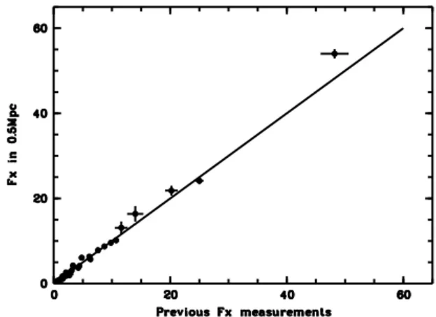
Fig. 5. Previous and present cluster flux (in a 0.5Mpc radius) comparisons.
The agreement is very good for the [0.5-2 keV] fluxes mea-sured in a 500kpc radius (Fig. 5).
For the Subaru Deep Survey region, we compared our detections with the extended X-ray source catalog of Ueda et al. (2008) and with the structure catalog of Finoguenov et al. (2010). Nine of our X-ray clusters are inside the area covered by these catalogs and six are also detected by these authors. Redshifts are always in very good agreement. Finoguenov et al. (2010) list in their paper 57 structures in-side this area. However, their selection function (complete-ness/contamination) for the X-ray extended sources as well as the characteristics of these sources (extent-measurement along with error or likelihood) are not published, thus preventing any meaningful comparison between the two samples. Moreover, as shown by Pacaud et al (2006) a flux limit, unless it is set very high, cannot define a complete uncontaminated sample of extended sources.
We finally performed a comparison with independently op-tically detected clusters in the literature. Limiting ourselves to studies giving a galaxy velocity dispersion estimate, we have five detections in common with Hamana et al. (2009: see Table 2). All these clusters are C1 structures. Redshifts are always in good agreement. Galaxy velocity dispersions are also consistent within error bars with an exception for XLSSC 050 where we find 408±96 km/s and where Hamana et al. (2009) find 739+150−86 km/s. This structure being very complex, the galaxy velocity dispersion is however very dependent on the selected galaxies and on the exact center choice.
4.4. Updated X-ray luminosities
We apply the principle of ”aperture photometry” to the flux measurement of the X-ray clusters, which avoids any other as-sumption than spherical symmetry as to the cluster shape. We note that Pacaud et al. (2007) used a beta-model fitting, which is not possible for the larger sample presented here, that com-prises faint objects. For these C2 and C3 objects, having some-times at most some hundred counts, it is not possible to perform a semi-interactive spatial fit as in Pacaud et al (2007), i.e.
let-Adami et al.: Optical assessment and comparative study of the C1, C2, and C3 cluster classes 7
Fig. 6. Redshift distribution for the 3 classes C1 (black his-togram), C2 (red hishis-togram), C3 (blue histogram).
ting the core radius and the beta value as free parameters. The resulting uncertainty would be very large.
We integrate the count rate in concentric annuli and derive the uncertainties by using Poisson statistic. Then, considering the count rate in each annulus, we stop the integration at the radius of the annulus for which the corresponding count-rate increase is comparable to the background 1-sigma fluctuation. This program operates in semi-interactive mode leaving the possibility to optimize the determination of the X-ray centroid and of the background level. The measurement yields for each cluster the total MOS1 + MOS2 + PN count-rate within a ra-dius 500 kpc. The fluxes have been obtained assuming a fixed conversion factor into the [0.5-2] keV band using a constant conversion factor of 9×10⁻¹³[(ergs/cm2/s)/(cnts/s)]. This value was calculated using Xspec from an APEC emission model with the following parameters: z=0.5, T=2 keV, Nh=2.6×1020 cm−2, Ab=0.3. Bolometric luminosities (also within a 500kpc radius) listed in the tables were also calculated with Xspec from the measured fluxes using the Pacaud et al. (2007) and the Bremer et al. (2006) temperatures when available. We used redshifts described in the next section. For clusters not listed in these papers (probably low mass structures), we used T=1.5 keV.
5. Global properties of the various classes
We will consider from this section to the end of the paper only clusters successfully identified.
5.1. Rich and poor structures
For X-ray sources unambiguously identified with optical veloc-ity structures, one has then to address the question: has the C1, C2, C3 classification a physical basis, or is it only reflecting the X-ray selection process?
As a first step, we look at the redshift distribution of the cluster C1, C2, and C3 classes (Fig. 6). For the 32 C1, the 9 C2, and the 17 C3 the mean redshift is 0.41, 0.66, and 0.38.
Comparing the C1 and C3 distributions and their almost similar mean redshifts and letting aside for a while the z ≥ 0.5
Fig. 7. Redshift distribution for the most luminous (Most l.),
luminous (L.), moderately luminous (Mod. l.), and C0 clusters.
C3 structures, it is tempting to consider C1 to be in the most cases ”X-ray bright and optical nearby (z ≤ 0.4) rich systems” and most of the C3 as ”faint and poor” at z ∼ 0.4 redshift. The more distant C3 clusters would be rather distant C1-like and therefore ”rich”. C2 clusters would be a mix of nearby poor and distant rich clusters.
We can define alternative categories to the C1, C2, C3 clas-sification. For instance, we chose to group the clusters as a function of their X-ray luminosity. Clusters more luminous than 1044 erg/s were called the X-ray most luminous sample. Clusters between 1043 and 1044 erg/s were called the X-ray
luminous sample. Clusters below 1043erg/s were called the
X-ray moderately luminous sample. Finally, clusters without any X-ray detection (C0 clusters) were considered separately. We give in Fig. 7 the redshift distribution of these 4 categories. As expected because of the relatively small angular coverage of the XMM-LSS survey, the most luminous clusters are mainly dis-tant objects. Similarly, moderately luminous clusters are quite nearby objects because our X-ray selection function does not allow us to detect them when they are distant, according to the well known Malmquist bias.
We show in Fig. 8 a synthethic view of the clusters listed in Tables 2, 3, and 4 allowing the reader to visualize the different classes (C1, C2, C3, most luminous, luminous, and
moderately luminous) in a redshift versus X-ray luminosity
di-agram.
5.2. Optical richness
We know (e.g. Edge & Stewart 1991) that optical and X-ray cluster properties should be relatively well correlated. It is then necessary to characterize the optical richness (NRich) of our
clusters. This is done by taking first the number of galaxies in the region of 500 kpc (radius), within the photometric redshift slice zmean ± 0.04 (1+z) and with magnitude less than m∗+ 3.
That number is then corrected by the ”field contribution” esti-mated in the same manner within 1 Mpc to give the final es-timate. This richness value is probably not accurate enough in terms of absolute value, but can be used in a relative way when comparing a structure to another one. We also note that, given
8 Adami et al.: Optical assessment and comparative study of the C1, C2, and C3 cluster classes
Fig. 8. Present paper cluster distribution in a log10(LX)
ver-sus redshift diagram. The two vertical green lines separate the
most luminous, luminous, and moderately luminous clusters.
Black disks are C1 clusters, red disks are C2 clusters, blue disks are C3 clusters. We also show as black, red, and blue curves the detection limit of the lowest X-ray flux cluster in C1, C2, and C3 classes.
the CFHTLS wide magnitude limit we adopted (i’=23), only z≤0.5 clusters are sampled deeply enough to reach m∗+ 3. We therefore only considered these clusters in order to avoid to have biased optical richnesses.
Fitting a richness-velocity dispersion for all z≤0.5 struc-tures for which both data were available, we get: log(σ) = (0.45 ± 0.24) log(NRich) + (1.96 ± 0.38).
This is compatible, within the uncertainties, with the value of Yee and Ellingson (2003), for similar kind of data:
log(σ) = (0.55 ± 0.09) log(Bcg) + (1.26 ± 0.30).
We now test richness and velocity dispersions versus X-ray properties. We first consider z≤0.5 structures with known X-ray luminosity and optical richness. We selected only C1, C2 and C3 clusters with X-ray luminosity at least two times larger than the associated uncertainty. We show in Fig. 9 the possible relation between the logarithm of NRichand of Lx. The linear
re-gression between the two parameters has a slope of 0.84±0.51. We note that this value only appears poorly significantly differ-ent from a null slope.
There is a single clear interloper: XLSSC 006 at z∼0.43 (outside of the box shown in Fig. 9). This is one of the most massive clusters in our sample. The observed spectra in the cluster center do not show any sign of AGN activity, so we have no reason to believe that the X-ray flux is polluted by a point source. This cluster shows signs of major substructures in the velocity distribution and this may explain its relatively high Lx value compared to its optical richness. Resulting compres-sion in the intracluster medium could increase the gas density resulting in an enhanced X-ray luminosity.
Considering now clusters at z≤0.5 with a known X-ray tem-perature (from Pacaud et al. 2007) and a measured galaxy ve-locity dispersion, we searched for a relation between NRich,
ve-locity dispersion, and X-ray temperature. Fig. 10 shows the re-lation between log(NRichσ2) and log(TX). We expect a linear
relation as (NRichσ2) is at least a qualitative measurement of
Fig. 9. log(NRich) versus log(LX). Crosses are clusters at signal
to noise lower than 2 regarding the X-ray luminosity. Disks are clusters at signal to noise greater than 2 and at z≤0.5 (black: C1, red: C2, blue: C3). They give the following fit: log(NRich) =
(0.84 ± 0.51) log(LX) + (7.2 ± 0.81).
the kinetic energy of the clusters, therefore close to the X-ray temperature. Error bars on (NRichσ2) are 68% uncertainties and
are computed assuming a perfect knowledge of the richness and the error bars on σ2given in Tables 2, 3, and 4. As quoted in Table 2, these uncertainties are computed with a bootstrap technique.
We have two outliers: XLSSC 027 and XLSSC 018. XLSSC 027 is known to have strong discrepancies be-tween galaxy and weak lensing equivalent velocity dispersions (898+523
−527km/s from Gavazzi & Soucail (2007) against 323±78 km/s for our own galaxy velocity dispersion and 447+82
−52km/s for the Hamana et al. (2009) galaxy velocity dispersion). We note that using the weak lensing equivalent velocity dispersion puts XLSSC 027 close to the best fit relation. We also note that this cluster has close contaminants at z=0.31 and 0.38 detected along the line of sight. This could also affect the measurement of the optical richness via the background estimate.
XLSSC 018 (without any sign of major substructures: see below) would need a larger optical richess and/or a larger galaxy velocity dispersion, or a lower X-ray temperature to fall on the best fit relation. The last solution in unlikely as only an X-ray temperature of the order of 0.4 keV would place XLSSC 018 on the best fit relation. A possible explanation would be that we are dealing with a structure close to a fossil group (even if it does not satisfy the characteristics of this class of structures). A significant part of the cluster member galaxies could have merged with the central galaxy, then depopulating the ≤m∗ + 3 magnitude range and diminishing the measured
optical richness.
In conclusion, and despite a few detected interlopers, the global agreements show the statistical reliability of our optical richness and galaxy velocity dispersion estimates.
Fig. 11 shows the histograms of the richness for the 3 classes. C1 has a mean NRichof 45, C2 a mean NRichof 37 and
Adami et al.: Optical assessment and comparative study of the C1, C2, and C3 cluster classes 9
Fig. 10. log(NRichσ2) versus log(TX) for the z≥0.5 clusters (all
C1 but XLSSC 046 which is C2). The + sign indicates XLSSC 027 and translates to the red disk when replacing the galaxy ve-locity dispersion by the weak lensing estimate from Gavazzi & Soucail (2007). The continuous line is the fit (computed with-out XLSSC 027 and XLSSC 018): log(NRichσ2) = (1.05 ±0.13)
log(TX) + (7.05 ± 0.07).
5.3. Substructure level in velocity space
Our spectroscopic catalogs are generally too sparse to allow precise substructure analyses. However, limiting ourselves to the confirmed clusters with available CFHTLS data and with more than 9 redshifts in the structure (10 clusters: XLSSC 013, XLSSC 025, XLSSC 022, XLSSC 006, XLSSC 008, XLSSC 001, XLSSC 000, XLSSC 018, XLSSC 044, and XLSSC 058), we applied the Serna-Gerbal method (Serna & Gerbal, 1996: SG hereafter) to these spectroscopic catalogs. Two of them (XLSSC 006 and XLSSC 001) are from the most luminous cluster category. All the others (but XLSSC 000 which is a C0 cluster) are members of the luminous cluster category. The SG method is widely used in order to characterize the substructure level in clusters of galaxies (e.g. Adami et al. 2009). Basically, the method allows galaxy subgroups to be extracted from a cat-alog containing positions, magnitudes, and redshift, based on the calculation of their relative binding energies. The output of the SG method is a list of galaxies belonging to each group, as well as information on the binding energy, and mass estimate of the galaxy structures.
The spectroscopic catalogs being still relatively sparse, we will only be able to detect very prominent substructures, but this is a good way for example to check if the analysed clusters are in the process of a major merging event.
Over the 10 analysed clusters, only two (which both belong to the most luminous cluster category) present sign of substruc-tures (XLSSC 006 with two dominant galaxies in its center and XLSSC 001) with 2 detected sub-groups. We checked if these two clusters were atypically sampled in terms of num-ber of available redshifts. XLSSC 001 has 17 redshifts and XLSSC 006 16 redshifts. Three other clusters without detected signs of substructures are equally sampled: XLSSC 013 has 19 redshifts, XLSSC 022 has 15 redshifts, and XLSSC 044 has 17 redshifts. The substructure detection therefore does not seem to be entirely due to selection effects depending on the
available number of redshifts. As a conclusion, all the tested
most luminous clusters show signs of substructures while none
of the other tested clusters show similar signs. This would be in good agreement with the most massive clusters being reg-ularly fed by their surrounding large scale structure in terms of infalling groups. Less luminous clusters would already be close to their equilibrium, with a less intense infalling activity. This has, however, to be confirmed with larger spectroscopic samples.
5.4. Relation between XMM-LSS clusters and their parent cosmic web portion
The previous subsection naturally raises the question of the characteristics of cosmological surrounding filaments. Numerical simulations place clusters of galaxies at the nodes of the cosmic web. Clusters are then growing via accretion of matter flowing along the cosmic filaments. This unquestion-able scenario for massive clusters is less evident for low mass structures as groups. Such groups could also form along the cosmic filaments as for example suggested for fossil groups by Adami et al. (2007a). Moreover, even for the most massive structures, the precise process of filament matter accretion is assessed most of the time only by individual cluster studies (e.g. Bou´e et al. 2008). The XMM-LSS cluster sample pre-sented in this paper offers a unique opportunity to investigate the cluster-filament connection with a well controled sample.
5.4.1. General counting method
We first have to detect the filaments connected to a given clus-ter. These filaments are very low mass and young dynamical structures. It is therefore very difficult to detect them through X-ray observations. This is possible only in a few peculiar cases (e.g. Bou´e et al. 2008, Werner et al. 2008) and with very long integration times. The XMM-LSS exposure times are any-way not well suited to such detections. We, therefore, used op-tical CFHTLS photometric redshift catalogs.
1 0 A d am i et al .: O p tic al as se ss m en t an d co m p ar at iv e st u d y o f th e C 1 , C 2 , an d C 3 cl u st er cl as se s
Table 2. List of the XMM-LSS C1 systems having successfully passed the spectroscopic identification. Name refers to the official IAU name. XLSSC refers to the official
XMM-LSS name. PH gives the availability of CFHTLS T0004 photometric redshifts: 0/1= not available/available. RA and DEC are the decimal J2000 coordinates of the X-ray emission center. N is the number of galaxies with spectroscopic redshifts belonging to the identified structure and within a radius of 500 kpc. ZBWT is the biweight estimate of the mean redshift of the structure (at a 0.001 precision). ERRZ is the upper value of the bootstrap uncertainty on ZBWT, at a precision of 0.001. It was computed only when more than 5 redshifts were available. SIG-GAP is the ”Gapper” estimate of the velocity dispersion given in km/s. ERR is the bootstrap uncertainty on SIG (computed when ≥5 redshifts were available). Flux is the value of the [0.5;2] keV flux in 0.5Mpc (radius) in 10−14ergs/cm2/s. Lx is the bolometric (0.1 to 50 keV) X-ray luminosity (in 1043erg/s) derived from the observed flux. NNPis the net number of photons in 0.5 Mpc. The two last columns give name and redshift (when available) when the considered cluster was also detected by Hamana et al. (2009), Ueda et al. (2008), or Finoguenov et al. (2010). When coming from Hamana et al. (2009), the cluster name has the SL Jhhmm.mddmm format. When coming from Ueda et al. (2008), the cluster name refers to this paper (4 digits number). When coming from Finoguenov et al. (2010), the cluster name refers to this paper (with the SXDF root). The * symbols indicate that the cluster validation was made with one or two spectroscopic redshifts. The (l) attached to the cluster id means that we have a lack of precision in the measured galaxy redshifts, preventing us to compute uncertainty of the mean cluster redshift, and velocity dispersions.
Name XLSSC PH RA DEC N ZBWT ERRZ SIG ERR Flux [0.5;2]keV LBol NNP Lit Id Lit z
deg deg km/s km/s 10−14ergs/cm2/s 1043erg/s
in 0.5Mpc in 0.5Mpc in 0.5Mpc XLSSU J021735.2-051325 059 1 34.391 -5.223 8 0.645 0.001 513 151 1.6±0.3 6.0±1.1 104±19 SXDF69XGG/0514 0.645 XLSSU J021945.1-045329 058 1 34.938 -4.891 9 0.333 0.001 587 236 2.0±0.2 1.5±0.1 601±54 SXDF36XGG/1176 0.333 XLSS J022023.5-025027 039 0 35.098 -2.841 4 0.231 2.2±0.4 0.7±0.1 183±34 XLSS J022045.4-032558 023 0 35.189 -3.433 3 0.328 4.1±0.4 3.1±0.3 465±43 XLSS J022145.2-034617 006 1 35.438 -3.772 16 0.429 0.001 977 157 24.1±0.8 46.0±1.6 1409±52 XLSS J022205.5-043247 040* 1 35.523 -4.546 2 0.317 2.0±0.3 1.4±0.2 265±35 XLSS J022206.7-030314 036* 0 35.527 -3.054 2 0.494 10.2±0.5 23.8±1.3 551±32 XLSS J022210.7-024048 047 0 35.544 -2.680 14 0.790 0.001 765 163 1.4±0.3 9.7±1.9 92±18 XLSS J022253.6-032828 048* 0 35.722 -3.474 2 1.005 1.1±0.2 13.1±2.9 81±18 XLSS J022348.1-025131 035* 0 35.950 -2.858 1 0.069 6.1±0.6 0.2±0.1 478±48 XLSS J022356.5-030558 028 0 35.985 -3.100 8 0.296 0.001 281 46 2.0±0.4 1.1±0.2 177±31 XLSS J022357.4-043517 049* 1 35.989 -4.588 1 0.494 1.9±0.2 3.9±0.5 287±34 XLSS J022402.0-050525 018 1 36.008 -5.090 9 0.324 0.001 364 69 1.7±0.2 1.3±0.1 382±44 XLSS J022404.1-041330 029(l) 1 36.017 -4.225 5 1.050 3.1±0.2 43.7±3.1 323±24 XLSS J022433.8-041405 044 1 36.141 -4.234 17 0.262 0.001 483 100 2.6±0.3 1.1±0.1 510±54 SL J0224.5-0414 0.2627 XLSS J022456.2-050802 021 1 36.234 -5.134 7 0.085 0.001 231 64 4.2±0.7 0.1±0.1 664±115 XLSS J022457.1-034856 001 1 36.238 -3.816 17 0.614 0.001 940 141 7.8±0.4 29.3±1.6 671±36 XLSS J022520.8-034805 008 1 36.337 -3.801 11 0.299 0.001 544 124 1.8±0.4 1.0±0.2 196±39 XLSS J022524.8-044043 025 1 36.353 -4.679 10 0.266 0.001 702 178 8.7±0.5 4.2±0.2 1098±62 SL J0225.3-0441 0.2642 XLSS J022530.6-041420 041 1 36.377 -4.239 6 0.140 0.002 899 218 21.8±1.1 2.2±0.1 1143±62 SL J0225.4-0414 0.1415 XLSS J022532.2-035511 002 1 36.384 -3.920 8 0.772 0.001 296 56 2.6±0.3 16.4±1.7 238±25 XLSSU J022540.7-031123 050 0 36.419 -3.189 13 0.140 0.001 408 96 54.0±1.1 7.8±0.2 4929±103 SL J0225.7-0312 0.1395 XLSS J022559.5-024935 051 0 36.498 -2.826 6 0.279 0.001 369 99 1.1±0.3 0.5±0.1 160±41 XLSS J022609.9-045805 011 1 36.541 -4.968 8 0.053 0.001 83 16 13.1±1.5 0.2±0.1 1706±192 XLSS J022616.3-023957 052 0 36.568 -2.665 5 0.056 0.001 194 60 16.4±1.8 0.2±0.1 1297±146 XLSS J022709.2-041800 005* 1 36.788 -4.300 2 1.053 1.0±0.1 13.4±1.8 165±23 XLSS J022722.4-032144 010 0 36.843 -3.362 5 0.331 0.001 315 56 5.7±0.4 4.7±0.4 459±38 XLSS J022726.0-043216 013 1 36.858 -4.538 19 0.307 0.001 397 58 2.6±0.3 1.5±0.2 374±48 XLSS J022738.3-031758 003 0 36.909 -3.299 9 0.836 0.001 784 189 3.7±0.4 29.0±3.1 196±22 XLSS J022739.9-045127 022 1 36.916 -4.857 15 0.293 0.001 535 106 9.6±0.3 5.5±0.2 1741±58 XLSS J022803.4-045103 027 1 37.014 -4.851 6 0.295 0.001 323 78 6.3±0.4 4.2±0.3 653±41 SL J0228.1-0450 0.2948 XLSS J022827.0-042547 / 012 1 37.114 -4.432 5 0.434 0.002 726 95 3.4±0.3 4.7±0.4 444±37 XLSS J022827.8-042601
A d am i et al .: O p tic al as se ss m en t an d co m p ar at iv e st u d y o f th e C 1 , C 2 , an d C 3 cl u st er cl as se s 1 1
Table 3. Same as Table 2 but for C2 XMM-LSS systems. XLSS J022756.3-043119 would require more spectroscopy for confirmation. XLSSC 009, 064, and 065 were
originally classified as C2, but would be classified as C1 using more recent pipeline version. The * symbols indicate that the cluster validation was made with one or two spectroscopic redshifts. The (l) attached to the cluster id means that we have a lack of precision in the measured galaxy redshifts, preventing us to compute uncertainty of the mean cluster redshift, and velocity dispersions.
Name XLSSC PH RA DEC N ZBWT ERRZ SIG ERR Flux [0.5;2]keV LBol NNP Lit Id Lit z
deg deg km/s km/s 10−14ergs/cm2/s 1043erg/s
in 0.5Mpc in 0.5Mpc in 0.5Mpc XLSSU J021658.9-044904 065 1 34.245 -4.821 3 0.435 1.1±0.4 1.6±0.6 50±18 285/287 XLSSU J021832.0-050105 064 1 34.633 -5.016 3 0.875 1.6±0.1 13.5±0.8 937±56 SXDF46XGG/829 0.875 XLSSU J021837.0-054028 063* 1 34.654 -5.675 2 0.275 4.1±0.5 2.0±0.2 255±32 XLSS J022303.3-043621 046 1 35.764 -4.606 8 1.213 0.001 595 121 0.7±0.1 14.0±3.2 82±19 XLSS J022307.2-041259 030 0 35.780 -4.216 5 0.631 0.001 520 158 0.6±0.1 2.1±0.4 129±27 XLSS J022405.9-035512 007 1 36.024 -3.920 5 0.559 0.001 369 179 1.2±0.3 3.2±0.7 113±25 XLSSU J022644.2-034107 009 1 36.686 -3.684 8 0.328 0.001 261 53 1.7±0.4 1.2± 0.3 87±21 XLSS J022725.1-041127 038 1 36.854 -4.191 4 0.584 0.1±0.1 0.4±0.3 31±28 XLSS J022756.3-043119* - 1 36.985 -4.522 2 1.050? 0.2±0.1 2.9±1.5 49±26
1 2 A d am i et al .: O p tic al as se ss m en t an d co m p ar at iv e st u d y o f th e C 1 , C 2 , an d C 3 cl u st er cl as se s
Table 4. Same as Table 3 but for C3 XMM-LSS systems. The ** symbols indicate that we merged by hand 2 groups separated by the gapper technique in the final analysis. The
last line (C555 class) is the new cluster (see text). The * symbols indicate that the cluster validation was made with one or two spectroscopic redshifts. The (l) attached to the cluster id means that we have a lack of precision in the measured galaxy redshifts, preventing us to compute uncertainty of the mean cluster redshift, and velocity dispersions.
Name XLSSC PH RA DEC N ZBWT ERRZ SIG ERR Flux [0.5;2]keV LBol NNP Lit Id Lit z
deg deg km/s km/s 10−14ergs/cm2/s 1043erg/s
in 0.5Mpc in 0.5Mpc in 0.5Mpc XLSSU J021651.3-042328* - 1 34.214 -4.392 1 0.273 0.6±0.3 0.3±0.2 58±32 XLSSU J021754.6-052655(l) 066 1 34.478 -5.447 6 0.250 0.3±0.3 0.1±0.1 68±59 SXDF85XGG/621 0.25 XLSSU J021842.8-053254 067 1 34.678 -5.548 5 0.380 0.001 847 279 1.0±0.4 1.0±0.4 84±34 SXDF01XGG/876 0.378 XLSSU J021940.3-045103* - 1 34.919 -4.852 1 0.454 0.8±0.2 1.2±0.3 193±44 XLSS J022258.4-04070 024 1 35.744 -4.121 5 0.293 0.001 452 98 1.3±0.2 0.7±0.1 254±41 XLSS J022341.8-043051 026 1 35.925 -4.514 3 0.436 1.6±0.2 2.2±0.3 255±34 XLSSU J022509.2-043239 037 1 36.286 -4.542 3 0.767 0.1±0.1 0.3±0.7 11±28 XLSSU J022510.5-040147 043** 1 36.294 -4.029 3 0.170 2.6±0.9 0.4±0.1 142±49 XLSS J022522.8-042649 042 1 36.345 -4.447 6 0.462 0.003 1009 257 0.6±0.2 0.9±0.3 111±33 XLSS J022542.2-042434 068 1 36.424 -4.410 4 0.585 0.2±0.2 0.5±0.6 23±28 XLSS J022610.0-043120 069 1 36.542 -4.523 8 0.824 0.001 398 114 -0.4±0.2 - -XLSSU J022627.3-050001 017 1 36.615 -5.003 5 0.383 0.001 352 132 1.5±0.4 1.6±0.4 134±35 XLSSU J022632.5-040314 014 1 36.635 -4.054 6 0.345 0.001 304 84 1.4±0.5 1.1±0.4 74±29 XLSSU J022632.4-050003 020 1 36.638 -5.007 3 0.494 2.0±0.4 3.8±0.8 159±32 XLSSU J022726.8-045412 070 1 36.860 -4.904 5 0.301 0.001 180 47 0.2±0.2 0.1±0.1 32±39 XLSS J022754.1-035100* - 1 36.974 -3.851 2 0.140 0.7±0.5 0.1±0.1 107±72 XLSSU J022828.9-045939 016* 1 37.121 -4.994 2 0.335 0.4±0.5 0.3±0.4 33±44 C555 - 1 36.375 -4.429 7 0.921 0.001 759 248 0.3±0.1 2.9±1.1 47±18
Adami et al.: Optical assessment and comparative study of the C1, C2, and C3 cluster classes 13
Fig. 11. Distribution of the optical richness for the 3 classes C1 (thin black), C2 (thick red), and C3 (thick blue).
- We first selected only clusters at z≤0.5 in order to be able to sample deeply enough the galaxy population to potentially detect the filaments, given the i’=23 magnitude limit for the photometric redshift catalog as demonstrated in Adami et al. (2010).
- For a given cluster, we selected galaxies with photometric redshifts in a 0.04×(1+z) slice around the cluster redshift.
- We then computed the number of galaxies in the slice in 72 angular sectors 10 degrees wide each, with position angles between 0 and 360 degrees. Each sector was overlapping the previous one by 5 degrees. We did this exercise for galaxies in a circle of 2.5Mpc radius, and in an annulus between 2.5 and 5 Mpc.
5.4.2. Filament detection and signal enhancement Intuitively, if a given sector is significantly more populated than other sectors, it means that this sector is including a galaxy overdensity which could be explained by a filament or by a group along a filament. The question is then to define a signifi-cance level. For a given cluster (and then a given redshift slice) and a given radius, we chose to compute the mean and disper-sion of the galaxy numbers in the 72 considered sectors. If a given sector had a number of galaxies larger than the mean + 3 times the dispersion, we considered this sector as hosting a potential cosmic filament portion.
However, individual clusters exhibit at best a single 3-σ significant candidate filament. This is due to the intrinsic very low galaxy density in filaments. Moreover, the goal of the present section is not to make individual cluster studies, but to draw statistical tendencies. In order to enhance the signif-icance of the filament detections, we therefore stacked differ-ent clusters, considering two categories: the luminous and the
moderately luminous clusters. Other categories did not have
enough cluster members in the selected redshift range. This technique is based on the assumption that the angular separa-tion between different filaments feeding a given cluster is more or less constant. In order to make such a stack we now need to homogeneize the cluster position angles. We chose the position angle of the highest galaxy overdensity (the PA), limiting
our-Fig. 12. Stacked X-ray images with position angles defined by the highest galaxy overdensities aligned along the 180deg ar-bitary angle. Images were rescaled to physical units accord-ing to cluster redshift. Image size is 1 Mpc×650 kpc. Contours were drawn with a 20×20 pixel smoothing. Upper figure: mean stacking. Lower figure: median stacking.
Fig. 13. Same as Fig. 12 with a median stacking and without any position angle correction.
selves to clusters exhibiting a detection more significant than the 3-σ level. Selected clusters were rotated to have their most significant filament at an arbitrary position angle of 180 degrees (east-west direction). In order to check if this alignment tech-nique has a physical meaning, we superposed in the same way the X-ray images using the position angles defined by the high-est galaxy overdensities (more significant than the 3-σ level). After rotating these X-ray images, we spatially rescaled them to physical units (kpc) according to redshift, and we simply added them together, taking into account the corresponding weight maps. The resulting point spread function is a mean of the in-dividual values and remains small compared to cluster typical sizes. Fig. 12 shows that we generate in this way a clearly elon-gated synthethic X-ray cluster along the 180deg direction. The measured ellipticity of the external isophote is equal to 0.41. If instead of a simple sum we compute the median of the im-ages (Fig. 12), the resulting ellipticity of the external isophote is still 0.36. Finally, if we combine the X-ray images without correcting by the optically determined orientation, we produce Fig. 13, showing a basically null ellipticity.
If the galaxy-defined prefered orientations are valid, the de-tected elongation in X-rays is an expected behaviour as X-ray emiting groups are also expected to fall onto clusters coming from surrounding filaments (see e.g. Bou´e et al. 2008).
We have to take into account the cluster redshift before merging their galaxy populations. A single catalog magnitude limit would evidently increase the weight of nearby clusters as compared to more distant ones. We therefore limited the galaxy catalogs to i’=23 at z=0.5. The limits were brighter by D mag-nitudes for nearer clusters with D being the distance moduli difference between the cluster redshifts and z=0.5.
Renormalizing finally the galaxy counts by the number of selected clusters in a given class, we are able to produce fig-ures giving the mean galaxy counts as a function of the angular position.
5.4.3. Results
We first draw stacked (using the previously defined PA of each cluster) angular galaxy counts for luminous and
moderately luminous clusters in the annulus [2.5,5]Mpc
(Fig. 14). The minimal and maximal radii have been choosen to be close to the mean virial radius of clusters (e.g. Carlberg et al. 1996) and not too large in order to limit the contamination by other clusters. These annuli will therefore mainly sample the infalling galaxy layers, just before the cluster dominated
14 Adami et al.: Optical assessment and comparative study of the C1, C2, and C3 cluster classes
Table 5. Same as Table 3 but for C0 clusters. An approximate upper limit for the X-ray luminosity of these clusters would be the faintest detected value for C3 clusters: ∼0.08 1043erg/s.
Name XLSSC PH RA DEC N ZBWT ERRZ SIG ERR
deg deg km/s km/s 022207.9-042808* - 1 35.533 -4.469 2 0.316 022402.4-051753 000 1 36.010 -5.298 11 0.496 0.001 435 88 022405.0-041612 - 1 36.021 -4.270 8 0.862 0.001 457 70 022528.3-041536 045 1 36.369 -4.261 4 0.556 022550.4-044500* - 1 36.460 -4.750 2 1.529 022647.5-041428* - 1 36.698 -4.241 1 0.742 022829.7-031257* - 0 37.124 -3.216 2 0.313
Fig. 14. Stacked angular galaxy counts (in arbitray units) for
luminous (black line) and moderately luminous (red line)
clus-ters in annuli of [2.5,5]Mpc. The horizontal lines show the 3-σ detection levels.
areas. As expected, the signal from the most significant fila-ment candidate is drastically increased, but no other features are detected at the 3-σ level besides the main filament.
We redo now the same exercise inside a 2.5 Mpc radius central area (Fig. 15). This area is mainly dominated by the clusters themselves (the few hundreds of kpc central areas) and by the galaxy layers just beginning to experience the cluster influence (close to the virial radius). We therefore investigate the cluster region as fed by the connected filaments. The sig-nal from the main filaments is still increased. Other significant filament candidates are detected at the 3-σ level mainly for the
moderately luminous cluster sample.
This difference between the 2.5 Mpc radius central area and the [2.5,5]Mpc annulus could be explained if the immediate vicinity of the considered clusters would be depopulated by the potential well of the clusters, diminishing the contrast between cosmic filaments and voids. Larger spectroscopic redshift sam-ples will soon become available in the area and will allow us to refine our results in future works.
6. Cluster galaxy populations characteristics
We now investigate the optical properties of the galaxy popula-tions in association with the X-ray clusters. We refer the reader
Fig. 15. Stacked angular galaxy counts (in arbitray units) for
luminous (black line) and moderately luminous (red line)
clus-ters inside a circle of 2.5 Mpc radius. The horizontal lines show the 3-σ detection levels.
to Urquhart et al. (2010) for individual studies of the clusters providing a temperature measurement.
6.1. Rest frame Red Sequences
The so-called red sequence (RS hereafter) commonly shows up to at least z∼1.2 (e.g. Stanford et al. 2002) in the massive structures. It is also detected in a less compact state in field galaxy populations up to z∼2 (Franzetti et al. 2007). We there-fore searched RSs in our sample of clusters. This sample does not provide enough statistics per cluster in order to perform in-dividual studies. The optimal strategy is therefore to build syn-thetic clusters by gathering galaxies for clusters of the same category. We therefore considered 4 classes of clusters: the
most luminous, the luminous, the moderately luminous, and
the C0 clusters. The RS being a powerful tool to characterize the evolutionary stage of the cluster galaxy populations (e.g. Adami et al. 2007b), such a study will allow us to assess the properties of these 4 cluster classes.
In order to be able to stack different clusters at different redshifts, rest frame absolute magnitudes were computed in the process of getting photometric redshifts with LePhare (e.g. Ilbert et al. 2006) and we used these magnitudes to compute colors. Basically the method consists in selecting the observed band which is the closest of the requested rest frame band to
Adami et al.: Optical assessment and comparative study of the C1, C2, and C3 cluster classes 15 compute the magnitude in this band applying correction
fac-tors. They are described in the annex of Ilbert et al. (2005), including for example k-correction. This method is the clos-est of the observations and minimizes our dependence on the assumed spectral energy distributions, which could not be ex-actly the same in clusters and in the field (see also annex I of the present paper).
6.1.1. Red sequence using spectrocopic redshifts In a first step we look only at galaxy members using spectro-scopic redshifts rather than photometric ones in order to re-move potential interloper galaxies which are non cluster mem-bers but close to the cluster redshift. Such galaxies could be interpreted as cluster members considering only photometric redshifts because of their limited precision. We here consider u*-r’ rest frame colours and look at their behaviour versus rest frame r’ absolute magnitude.
Fig. 16 shows that a RS is present with u*-r’∼2 for all clus-ters. The slopes of the RS appear in good agreement with litera-ture estimates (e.g. Adami et al. 2007b: between -0.1 and -0.02 for the Coma cluster) and are given in Table 6. As expected, RSs are populated by early type galaxies, while later type ob-jects are grouped in a much less compact bluer sequence.
There are potential differences between C0 clusters (with-out detectable X-ray emission) and other classes. The slope of the RS appears nearly flat for C0 clusters while being more neg-ative for more luminous clusters. This effect is only poorly sig-nificant when considering the uncertainty of the slope of these RS’s. We performed however a bi-dimensional Kolmogorov-Smirnov statistical test on the early type galaxies of Fig. 16. The probability that the C0 and the most luminous cluster early type galaxies come from the same population is only 0.6%. The probability that the C0 and the luminous cluster early type galaxies come from the same population is only 0.1%. Finally, the probability that the C0 and the moderately luminous clus-ter early type galaxies come from the same population is 3.1%. At least for the most luminous and luminous cluster popula-tions, early type galaxies therefore seem to be differently dis-tributed in a color magnitude relation compared to C0 cluster early type galaxies. If these differences come from the slope of the RS, this effect could be interpreted as a metallicity effect (Kodama & Arimoto, 1997). The more massive a galaxy, the more easily it will retain metals against dissipative processes. The more metals present in a galaxy, the redder the galaxy will be. Massive galaxies are therefore expected to be redder than lower mass objects. A possible explanation would be that the faint early type C0 cluster galaxies would originate from depleted cores of larger galaxies, so being metal rich before becoming faint (see e.g. Adami et al. 2006). This is possible for example in small groups where velocity dispersion is low enough to favor galaxy-galaxy encounters.
Galaxie members of the most luminous clusters also appear to exhibit a more pronounced dichotomy between early and late type objects. Blue members of the most luminous clusters are clearly bluer than blue members of the less luminous clusters.
Fig. 16. Rest frame u*-r’ versus absolute r’ magnitude rela-tion for clusters using spectroscopic redshifts to compute ab-solute magnitudes. We only plot cluster members in these fig-ures. From top to bottom, figures are for the most luminous, the luminous, the moderately luminous, and the C0 clusters. Red symbols correspond to early type galaxies (T ≤21), blue symbols correspond to late type non starburst galaxies (58≥
T ≥21), and pink symbols correspond to starburst galaxies
(T≥59). Black continuous lines are computed using only T ≤21 galaxies (see Table 6).
16 Adami et al.: Optical assessment and comparative study of the C1, C2, and C3 cluster classes
Table 6. Slopes of the red sequences for the four classes of clusters: most luminous, luminous, moderately luminous and C0. Category Slope most luminous -0.04±0.04 luminous -0.04±0.02 moderately luminous -0.10±0.04 C0 -0.01±0.05
6.1.2. Age of formation of the cluster galaxy stellar populations
We expect distant clusters to naturally exhibit younger galaxy star populations compared to nearby structures. In order to investigate this question, we computed with LePhare ages of stellar population in galaxies with a spectroscopic redshift ly-ing inside the considered clusters. The templates used to gen-erate public photometric redshifts in the CFHTLS does not allow to provide this information, so we used in LePhare the Bruzual & Charlot (2003) templates, fixing the redshifts to the spectroscopic values. The metallicity was let free to vary between 0.004, 0.008, and 0.02 Z⊙. In C0 clusters,
z=[0.3;0.6] galaxies have a stellar population aged of 6.2±1.9 Gyr, and z=[0.7;0.9] galaxies have a stellar population aged of only 2.7±1.3 Gyr. Considering members of luminous clus-ters, z=[0.25;0.35] galaxies have a stellar population aged of 7.4±1.0 Gyr, and z=[0.35;0.65] galaxies have a stellar pop-ulation aged of only 5.3±2.1 Gyr. Finally, members of the
most luminous clusters, z=[0.4;0.65] galaxies have a stellar
population aged of 5.2±2.1 Gyr, and z=[0.75;1.25] galaxies have a stellar population aged of 3.3±1.1 Gyr.
Taking the mean redshift of the highest redshift bin for each of these 3 categories and diminishing the corresponding elapsed time since the beginning of the Universe by the mean age of the early type galaxy stellar populations leads us to esti-mate the mean age of formation of the star populations in these galaxies. Galaxy stellar populations probably formed at z∼1.6 in C0 clusters, at z∼2 in luminous clusters, and at z∼2.5 in the most most luminous. These values are in good agreement with general expectations for the massive clusters to form early than low mass structures, up to redshifts close to z∼2.
6.1.3. Red sequence using photometric redshifts and color-color diagrams
In order to study larger samples and detect possible weak ef-fects, we used photometric redshifts to define a cluster mem-bership, and compute absolute magnitudes and colors as pro-vided by the CFHTLS data. Given its photometric redshift, a galaxy was assigned to a cluster when closer than 500 kpc from the cluster center and at less than 0.08 from the cluster redshift. This corresponds to the values quoted in Table A.1 for cluster galaxies. We then were able to search for RSs in the most luminous, the luminous, and the moderately luminous clusters. Selecting all available clusters in these three categories Fig. 17 clearly shows red sequences in each case. They all are
consistent with a u*-r’ color of 1.9, the most massive clusters exhibiting the more negative RS slope (computed with T ≤ 21 galaxies). On the contrary, the C0 clusters (no X-ray detection) only exhibit a very low number of early type galaxies (but still consistent with u*-r’∼1.9). These structures therefore appear as quite young structures, with modest early type galaxy popula-tions.
However, we are merging in Fig. 17 clusters with quite different redshifts and evolutionary effects could play an im-portant role. We therefore selected only the luminous clusters (the only category providing enough clusters) and we divided this population in 3 different redshifts bins (≤0.3, ]0.3,0.5], and ]0.5,0.8]) in Fig. 18. This figure only shows T ≤ 21 galaxies (early types). RSs appear very similar, with the most negative slope occuring for z=]0.5,0.8] clusters. If evolutionary effects are present, they are therefore rather weak, besides the most distant clusters appearing to have the most negative RS slope (-0.069±0.017). This is consistent with the slope computed for the most luminous clusters (which are also nearly all at redshift greater than 0.5): -0.052±0.015.
It could be argued that the use of photometric redshifts could introduce a bias due for example to SEDs not adapted to high density regions. In order to check the previous results, we therefore simply draw u*-r’ versus r’-z’ color-color dia-grams for the same sets of clusters. Fig. 19 shows that in both cases, early types still occupy well defined loci in the color-color space, confirming the existence of an old galaxy popula-tion in these cluster classes.
We therefore confirm that both massive and less massive X-ray structures in our sample exhibit quite similar red sequences, making them overall quite old structures. Non X-ray clusters are probably minor structures with a poor spectral early type population.
Fig. 17 also shows a slightly larger percentage of star-burst galaxies (as determined during the photometric redshift computation process: see Coupon et al., 2009) in low lumi-nosity clusters. C0, moderately luminous, and luminous clus-ters exhibit 20% more starburst galaxies compared to the
most luminous clusters. This is an expected behaviour, for
example in good qualitative agreement with Urquhart et al. (2010).
6.2. Luminosity Functions
In the same spirit, we checked whether our structures behave as genuine clusters or groups concerning their galaxy luminos-ity functions. For a detailed study of the individual XMM-LSS C1 cluster luminosity functions, we refer the reader to Alshino et al. (2010). We computed luminosity functions using galax-ies within the cluster bins (according to photometric redshifts). The Schechter function fitting was performed allowing a con-stant background to take into account galaxies included in the photometric redshift slice but not part of the clusters.
Selecting all clusters (C1+C2+C3+C0), stacking their lu-minosity functions, and only limiting absolute magnitude to i’≤-17.5 in order to not be too affected by incompleteness, we got a best fit of a Schechter function with alpha = -1.15±0.09