Quantifying microbial methane oxidation efficiencies in two experimental landfill biocovers using stable isotopes
Cabral, A.R.1,*, Capanema, M. A.1, Gebert, J.2, Moreira, J.F.1 and Jugnia, L.B.3
1 Dept. Civil Eng., Faculty of Eng., Univ. de Sherbrooke, Sherbrooke, QC, Canada, J1K 2R1 2 University of Hamburg, Institute of Soil Science, Allende-Platz 2, 20146 Hamburg, Germany 3 Biotechnology Research Institute, 6100, Royalmount Ave., Montreal, QC, Canada, H4P 2R2
*Corresponding author: Alexandre.cabral@usherbrooke.ca, +1 819-821-7906; +1-819-821-7974 (fax)
ABSTRACT
Stable isotope analyses were performed on gas samples collected within two instrumented biocovers, with the goal of evaluating CH4 oxidation efficiencies (f0). In each of the biocovers, gas probes were installed at four locations and
at several depths. One of the biocovers was fed with biogas directly from the waste mass, whereas the other was fed through a gas distribution system that allowed monitoring of biogas fluxes. While the f0 values obtained at a depth of
0.1 m were low (between 0.0 and 25.2%) for profiles with poor aeration, they were high for profiles with better aeration, reaching 89.7%. Several interrelated factors affecting aeration seem to be influencing f0, including the
degree of water saturation, the magnitude of the biogas flux, and the temperature within the substrate. Low f0 values
do not mean necessarily that little CH4 was oxidized. In fact, in certain cases where the CH4 loading was high, the
absolute amount of CH4 oxidized was quite high and comparable to the rate of CH4 oxidation for cases with low
CH4 loading and high f0. For the experimental biocover for which the CH4 loading was known, the oxidation
efficiency obtained using stable isotopes (f0 = 55.67% for samples taken inside flux chambers) was compared to the
value obtained by mass balance (f0 = 70.0%). Several factors can explain this discrepancy, including: the high
sensitivity of f0 to slight changes in the isotopic fractionation factor for bacterial oxidation, αox, uncertainties related
to mass flow meter readings and to the static chamber method.
1. INTRODUCTION
Methane (CH4) is a greenhouse gas with an infrared activity 25 times that of CO2 (IPCC 2007) and its
atmospheric concentration is increasing at a rate of 0.6% per year (IPCC 2001). Landfills represent an important source of CH4 emissions and, according to several sources (e.g. Bogner and Matthews 2003; De Visscher et al.
2004; Stern et al. 2007; Chanton et al. 2008), their contribution to the global CH4 emissions may vary from 3 to
10%. Therefore, management practices that could help reduce emissions from landfills are of great importance in connection with the atmospheric CH4 budget. Gas extraction systems, which are now widely adopted in the
developed world, are considered the principal means of achieving such reductions. However, gas collection systems are not 100% efficient; indeed, it has been reported that even at sites with gas collection systems, significant amounts of biogas can still escape as fugitive emissions (e.g. Spokas et al. 2006; Börjesson et al. 2007).
According to the Working Group III of the Intergovernmental Panel on Climate Change, one promising management strategy to reduce emissions from landfills is the installation of a biocover as part of the final cover system (IPCC 2007; Table SPM 3). When a final cover is engineered to optimize the growth and activity of the methanotrophic bacteria, it becomes a passive methane oxidation biocover (PMOB). In PMOBs, CH4 reduction is
regulated by methanotrophic bacteria that develop in the aerobic zone near the surface. The microbial oxidation of methane for the abatement of landfill methane emissions is not only applicable as a complement to gas extraction, but is also suited to treat residual emissions during aftercare or low calorific emissions from wastes that have a low gas generation rate.
Methanotrophs in landfill covers or biofilters are capable of converting CH4 to CO2 and biomass in the
presence of atmospheric O2 (e.g. Boeckx et al. 1996; Humer and Lechner 1999; Boeckx and Van Cleemput 2000;
Hilger and Humer 2003; Gebert and Gröngröft 2006; Stern et al. 2007). The process of microbial oxidation is influenced by several factors, including, among others, the temperature within the cover, the diffusivity of the cover material and the magnitude of biogas flux. The latter partly depends on the differential pressure between the waste mass and the atmosphere that also partly controls the availability of O2, and the air-filled porosity, which also
depends on the amount of water infiltration through the top cover.
Despite the promising future of biocovers, the reliability of methods to estimate CH4 oxidation efficiency of
biocovers in the field remains a problem. It is indeed difficult to estimate efficiencies without knowledge of the CH4
fluxes reaching the base of a cover and leaving it, moreover when emissions may span over 7 orders of magnitude (Bogner et al. 1997), and important variations in the magnitude of emissions may be found within the same landfill (Czepiel et al. 1996; Scheutz et al. 2003). A technique that has been recently employed in several field studies
estimates CH4 oxidation efficiency in landfill covers based on changes in the ratio of two stable carbon isotopes,
namely 13C and 12C (Liptay et al. 1998; Chanton and Liptay 2000; De Visscher et al. 2004; Chanton et al. 2008).
While 12C is 99% abundant, 13C responds for the remaining 1%.
This paper presents the results obtained from the stable isotope analysis performed on gas samples collected during the 2007 monitoring campaign of two PMOBs installed at the St-Nicéphore landfill, Quebec, Canada, a waste disposal facility covering approximately 65 hectares that receives mainly domestic waste. The goal was to estimate the biotic methane oxidation efficiencies of the two PMOBs. Gas samples were frequently taken at several locations and depths within the PMOBs. For clarity, the main design characteristics of the PMOBs and the instrumentation installed are described.
2. BACKGROUND
The carbon stable isotope composition is expressed as follows (e.g. Chanton et al. 1999):
1000
1
)
‰
(
tan 13
dard s sampleR
R
C
(1)where Rsample is the 13C/12C ratio of the sample and Rstandard is the 13C/12C ratio of the reference standard VPDB
(Vienna Peedee Belemnite; Rstandard = 0.01124).
Studies using methanotrophic cultures have shown that the lighter isotope 12C is oxidized more rapidly than
the heavier isotope 13C, (Chanton and Liptay 2000; De Visscher et al. 2004). As a result, changes in isotope
composition occur when methane is oxidized, altering the isotope ratio. Indeed, δ13C values of CH4 produced in the
deepest zone of the landfill profile are typically between - 50 and - 61‰, and the δ13C values of emitted CH4 are
generally between -30 and -50‰ (Chanton et al. 1999). Knowledge of δ13C values of the CH4 produced and emitted
allows calculating the fraction of methane that is oxidized when fugitive emissions of biogas migrate through the top cover (De Visscher et al. 2004). The percentage of CH4 oxidized (or oxidation efficiency, f0) is determined by the
following equation (taken from Abichou et al. 2006a):
A E
α
α
δ
δ
0.1
0f
(2)where δA is the δ13C value of the anoxic zone; δE is the δ13C value of emitted CH4; αox is the isotopic fractionation
factor for bacterial oxidation; and αtrans is the isotopic fractionation factor associated with gas transport.
The fractionation factor for microbial oxidation αox can be obtained empirically (Liptay et al. 1998; De
Visscher et al. 2004). Previous studies pertaining to landfill emissions reported different values of αox, some of
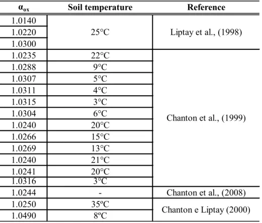
which are summarized in Table 1 (with the associated temperatures prevailing when the samples were taken). The variation of soil temperature modifies the fractionation factor value and, therefore, the calculated methane oxidation efficiency. Tyler et al. (1994) presented a temperature-dependent variation of αox = 0.00046/K, with increasing
temperatures causing a decrease in αox, thus an increase in f0. In a seasonal variation study, Chanton and Liptay
(2000) obtained the following dependence relationship: αox = 0.000435/oC, where αox varied between 1.025 (at 35oC)
and 1.049 (at 8oC), with the latter being among the greatest values found in the literature.
According to the study by Chanton and Liptay (2000), αox does not vary as a function of soil texture. Liptay et
al. (1998) also reported that differences between clayey and sandy soils didn’t affect the αox value, despite varying
oxidation efficiencies. Tyler et al. (1994) observed that moisture content affected the αox value.
The isotopic fractionation factor associated with gas transport (αtrans) is assumed to be 1.0, which supposes that
CH4 transport across the PMOB is dominated by advection (Liptay et al. 1998; Abichou et al. 2006b; Stern et al.
2007), a process that does not cause isotopic fractionation (Liptay et al. 1998). Recent laboratory experiments by De Visscher et al. (2004) have shown that this approach can underestimate CH4 oxidation by not taking into account
diffusive flux, which can play a significant role in gas transport. If diffusive transport becomes important, then αtrans
would be greater than 1. However, several authors (including De Visscher et al. 2004; and Stern et al. 2007) cite the works of Czepiel et al. (1996; 2003) who claim that the assumption of a preponderance of advective flux is supported by observations of a strong negative relationship between CH4 emission and atmospheric pressure at
several landfills. This is particularly true for landfill sites without gas collection systems.
3. Materials and Methods
Experimental plots
Three experimental plots measuring 2.75 m (W) × 9.75 m (L) were constructed with a slope of 3.5%, in the middle of an already capped area of the St-Nicéphore landfill. The final cover in this area was constructed with a
thick (almost 3 m in certain areas) layer of silt placed directly on the waste mass (as required by law). In this paper, only details pertaining to two PMOBs, namely PMOB-1 and PMOB-3B, are presented.
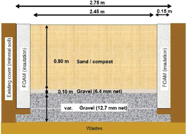
PMOB-1 included a 0.80 m thick layer of substrate underlain by a 0.10 m thick transitional layer consisting of 6.4-mm clean gravel and a 2.0- m thick gas distribution layer (GDL) consisting of 12.7-mm clean gravel. This plot was fed directly by biogas coming from the 3.5-year old buried waste mass (Fig. 1). As a result, it was not possible to control (or to obtain) the upward flux of biogas. The substrate layer consisted of a mixture of sand and compost, composed of 5 volumes of compost (before sieving) and 1 volume of coarse sand (D10 = 0.07 mm; D85 = 0.8 mm).
More details on the compost and the mixture can be found in Jugnia et al. (2008). The substrate layer was placed in four 0.2-m layers and compacted with a vibrating plate to obtain layers with an average density of 8.4 kN m-3 and
total porosity (n) equal to 0.63. The specific density of the solids (Gs) of the sand-compost mixture is equal to 22.5
kN m-3.
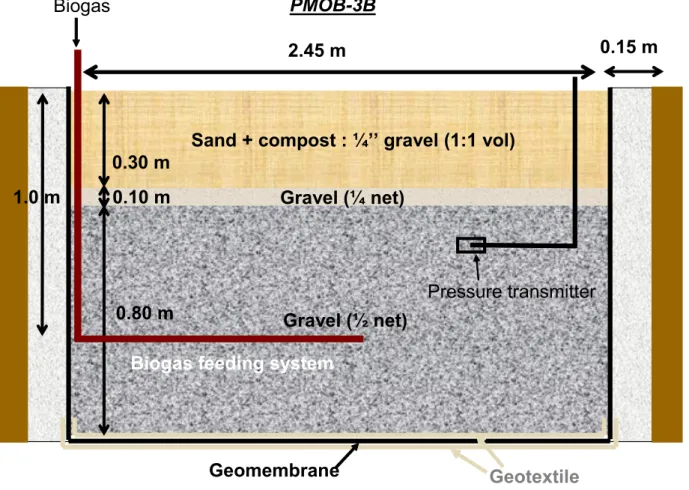
PMOB-3B (Fig. 2) was constructed using a coarser substrate that resulted from mixing one volume of the same material used as substrate in PMOB-1 with one volume of 6.4-mm gravel. The 0.3-m thick substrate was compacted to a density of 14.0 kN m-3 and total porosity equal to 0.48. The GDL included 0.10 m of 6.4-mm clean gravel as a
transitional layer and 0.80 m of 12.7-mm clean gravel layer. Contrary to PMOB-1, PMOB-3B was lined with a 1-mm thick HDPE geomembrane (GM), protected against tearing by a geotextile sheet. This completely isolated this experimental plot from the existing silty cover and the waste mass. PMOB-3B was fed with biogas from a well installed exclusively for this study. The amount of biogas fed into the system was controlled by means of a valve and the flow could be monitored by a mass flow meter connected to a data acquisition system. A drainage system was installed at the lowest point to evacuate infiltrating waters.
The walls around each of the two PMOBs were thermally shielded from the outside environment by 0.15-m thick polystyrene panels. The goal was to prevent lateral migration of moisture due to thermal gradients, which could lead to preferential flow paths. Temperature sensors (TMC20-HD, from Onset), connected to a data acquisition system (HOBO U12, from Onset) and gas probes (aluminum tubes with an inner diameter of 10 mm that were capped at the top end with a septum) were permanently installed at 4 separate downgradient points and at 4 different depths (6 depths in the case of gas probes) in each profile (Fig. 3), making up for a total of 48 gas probes and 32 temperature sensors for the two PMOBs. Tensiometers (Low Tension Irrometer, from Irrometer Company) and water content sensors (EC-5, from Decagon) were also installed and connected to data acquisition systems, allowing for the determination of the degree of saturation. The temperature and water content probes were
connected to data loggers. Meteorological data, including air temperature, precipitation, atmospheric pressure and wind speed were continuously recorded by a weather station installed near the experimental plots.
Gas analyses
For each gas probe in a profile, gas samples were taken on a weekly basis. The equivalent to the volume of the aluminum tubes was initially purged using the same syringe that one hour later was again introduced through the septum to collect the gas sample. The volumetric concentrations of CH4, CO2 and O2 in the collected samples were
obtained using a portable landfill gas analyser (Portable Gas Meter, Columbus Instruments, OH) equipped with infrared sensors able to detect CO2 and CH4. It also has an electrochemical sensor able to detect the volumetric
concentration of O2.
In mid summer of 2007, samples were also collected at a depth of 0.05 m using a specially designed gas probe that was manually inserted in the soil at every sampling date. Due to the small volume of biogas collected at this depth, gas samples were stored in a vacutainer serum tube and analysed within 24 hours in the laboratory using a gas chromatograph (Agilent 3000A Micro GC, equipped with a TCD detector and two columns, Molsieve for CH4 and
O2 and Plot Q for CO2).
In order to draw concentration profiles, the CO2 and CH4 concentrations at the surface were assumed to be nil
due to dilution with atmospheric air (which does not mean that the CH4 surface fluxes were exactly equal to zero).
The O2 volumetric concentration in the air, at the surface, was assumed to be equal to 20.9%. The N2 concentrations
were not obtained by direct measurement, but calculated as the difference between 100% and the sum of the concentrations of the three other gases (CO2, O2 and CH4). As compared to O2, N2 is more relevant in indicating the
aeration level, because it is neither consumed by oxidation near the surface nor by soil respiration. This was calculated for each depth within the several profiles analysed.
Stable isotope analyses
Samples for stable isotope analyses were taken at selected dates and locations in order to study oxidation efficiencies of four types of profiles, which are presented in the Results section. Samples were usually taken from the deepest gas sampling tube – that contains raw landfill gas – and from the top-most gas tube (0.10 m; in one case, 0.05 m). For 3 selected profiles, samples were also taken from approximately mid-depth (0.3 or 0.4 m) of the substrate layer.
For all the selected dates, a sample for stable isotope analysis was taken during surface flux measurements, which were performed on a weekly basis at several locations at each of the plots, following the static chamber method, as described by Fécil et al. (2003). In the present study, the sample was taken while the concentration within the chamber was still increasing.
Isotope analyses were performed at the Delta-Lab (Geological Survey of Canada, GSC-Quebec). The GC-C-IRMS system consists of a HP 5890 Series II Gas Chromatograph (GC) coupled with a VG Prism III Isotopic Ratio Mass Spectrometer (IRMS) via a combustion interface VG Isochrom II. The GC column was a PoraPlot Q (Varian, CP-7551) plot-fused silica column (25 m, 0.32 mm). The results obtained were normalized (re-calculated versus VPDB) using three internal gas standards. Two of them (BISO-1, HISO-1) were mixtures of 0.25% of methane and air. These were calibrated versus VPDB at the University of Victoria, BC. The third gas, CO2 had a δ13C value
different from the reference gas. The latter was obtained from the BOC and calibrated versus VPDB at the Delta-Lab. The precision and accuracy for the standards were better than ± 0.4‰.
The fractionation factor for bacterial oxidation, αox, was calculated based on values found in the literature
pertaining to landfill emission studies (Table 1). Only values in the range of temperatures found during the present study were considered. The average αox value, 1.0235, was the one adopted. Since αox is temperature dependent, a
correction had to be applied (see Table 2) using Eq. (3), which is based on Tyler et al.’s (1994) temperature dependence relationship:
C)]
T(
0.00046[20
average
α
α
o ox ox
orα
ox
α
oxaverage
0.00046[29
3.15
T(K)]
(3)Eq. (3) shows that as temperatures rise above 20oC, lower values of αox are obtained, which, according to Eq.
(2), leads to higher oxidation efficiencies, f0.
4. RESULTS AND DISCUSSION
Gas concentration profiles
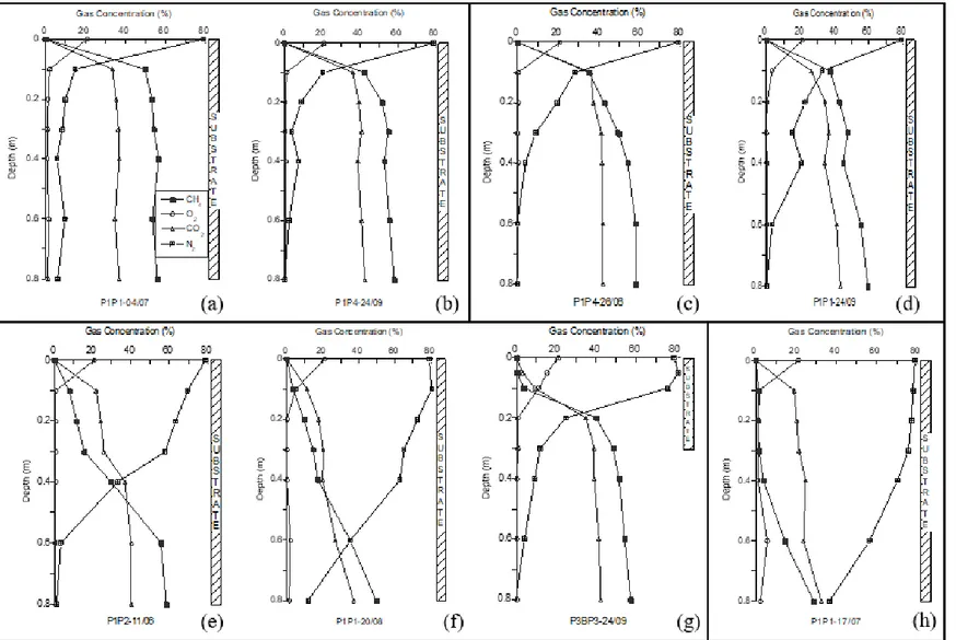
The gas concentration profiles corresponding to the dates when samples were selected for stable isotope analyses are presented in Fig. 4. Four types of typical profiles were identified and are described in the following.
Type 1 profiles (Fig. 4a, b) represent the periods during which the CH4 concentration did not change much as
biogas migrated up towards the atmosphere. This means that the system was not efficient in oxidizing the entire methane loading, at least up to the top-most gas sampling point, located 0.10 m below the surface. However, this does not mean that oxidation was not taking place. In fact, despite the poor CH4 oxidation efficiency, a significant
portion of the estimated CH4 loading was oxidized (Table 2). Above the 0.10 m point it is possible that further
oxidation may have taken place, but no monitoring was made to verify that.
Type 1 profiles can be associated with several factors affecting aeration of the substrate, including high degrees of water saturation, Sw, (and thus a decrease in air-filled porosity) and high upward biogas fluxes. The hypothesis of
high Sw near the surface for Type 1 profiles do not hold, because Sw values were similar to those found in other
situations where the oxidation efficiency was high (discussed below). The observed sharp decrease in N2 near the
surface (Fig. 4a,b) suggests poor aeration and points to high upward biogas loading as an important factor contributing to give the profile its shape. As far as evaluation of aeration is concerned, N2 is a better indicator than
O2 because it is neither consumed by oxidation near the surface nor by soil respiration. Although we did not have
any control on the magnitude of the CH4 loading (the GDL sits directly on the waste mass), an estimate of the
loading was made (see Table 2) based on loading data and the CH4 oxidation efficiency of the system, f0. The latter
is given by stable isotope data, which is presented and commented below.
With Type 2 (Fig. 4 c, d) the CH4 concentration didn’t change up to a depth of approximately 0.4 m, and then
decreased slightly, with the CH4 concentration at the uppermost sampling point (0.1 m), remaining high. The
observed deeper penetration of N2 associated with Type 2 profiles is an indication that the upper part of the substrate
was better aerated, which should favour oxidation. The surface flux obtained on Sept 24th was still high but much
lower than in the case of Type 1, which was consistent with the deeper penetration of N2. However, the quite high
flux obtained in all surface measurements made at PMOB-1 on June 26th (Table 2) is bewildering. Two possible
explanations can be offered: the first is that the locations of the profiles do not correspond exactly to the locations where surface flux measurements were conducted. In this case, the static chamber may have been placed exactly above a micro-fissure that was impossible to detect visually; as a consequence, a very high flux was measured. A second plausible cause for the high flux on June 26th is related to unequal moisture distribution within the substrate,
a phenomena associated with unsaturated flow of water through the cover, which may lead to heterogeneous (or non uniform) gas distribution within the PMOBs (Cabral et al. 2007). This, combined with potential preferential flow, may also explain the high flux measured.
While oxidation may be taking place near the surface, dilution of the pore gas also contributes to the decrease in CH4 concentration from 0.1 to the surface. In addition, part of the incoming O2 is consumed by soil respiration.
Type 3 (Fig. 4e, f, g) corresponds to profiles where a steady decrease in CH4 concentration was observed almost
throughout the substrate (note that the substrate for PMOB-3B starts at the 0.3 m mark; Fig. 4g), although the concentrations of CH4 at a depth of 0.1 m were still not negligible. One is tempted to associate these types of
profiles with favourable conditions leading to a much deeper penetration of atmospheric air (see N2 profiles in Fig.
4e, f, g), such as low degrees of saturation or increasing atmospheric pressure.The relatively high surface flux obtained on June 11th is also puzzling, given the quite effective penetration of atmospheric air. Finally, given the
greater potential for dilution near the surface and the surprisingly low O2 concentration below 0.1 to 0.2 m (in part
due to respiration), stable isotope data become an important tool to evaluate the actual oxidation efficiency of systems identified by these types of profiles.
The last one, Type 4 (Fig. 4h), represents profiles observed in PMOB-1 for nearly two consecutive weeks of dry weather, during the summer of 2007. Evidence of dryer substrate is found in the value of Sw at the bottom of the
substrate, which is the lowest of all shown in Fig. 5 for PMOB-1 (Sw = 82.1%). In addition, the surface flow was
below detectable limits and the nearly vertical N2 concentration profile (Fig. 4h) clearly indicates that the substrate
was well aerated throughout its depth. The CH4 concentration, which was already relatively low (28.8%) at 0.82 m,
decreased to quite low levels (~1%) at 0.3 to 0.4 m. The relatively high O2 concentration at 0.6 m may have resulted
from a measurement error; otherwise, the Authors cannot find any other plausible interpretation for this odd datum. The quite low concentrations of CH4 near the surface cannot be associated with oxidation alone. As mentioned
previously, soil respiration and dilution of the pore gas also have to be considered and stable isotope results become a useful tool to evaluate the extent of oxidation. Although it is impossible to verify (using either our data or site records), the CH4 loading might have been quite low during the two-week period during which the Type 4 profile
was obtained, allowing for the large extent of diffusive ingress of atmospheric air.
According to Chanton and Liptay (2000), and Stern et al. (2007), the optimum soil temperature for CH4
oxidation appears to be from 25 oC to 30 oC. With the exception of the profile obtained in PMOB-3B (Fig. 5g),
where temperatures remained in the vicinity of 30 ºC, for all the other dates for which sampling for isotope analyses was performed, the temperatures remained in the vicinity of 20 ºC. The lowest air temperature during the monitoring period was approximately 15 ºC and the highest reached approximately 30 ºC. For all sampling times, the air temperature (shown in Fig. 5 as the value at the surface) was always slightly lower than the temperature at 0.1 m.
δ13C Values and oxidation efficiencies
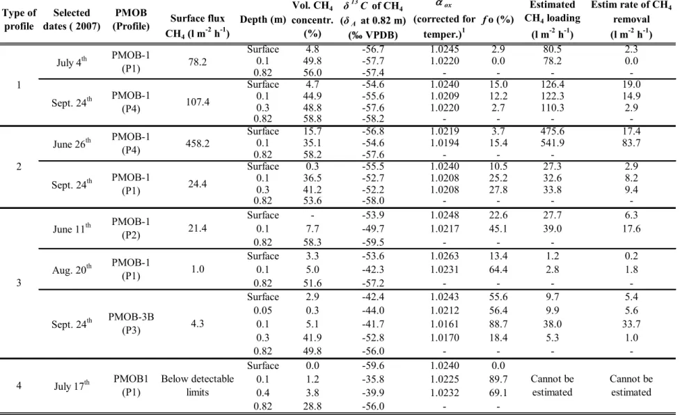
Table 2 presents the results of stable isotope analyses for the 4 types of profiles. The δ13C value of methane
from the waste mass (δA), or baseline CH4 concentration value, was obtained by applying Eq. (1) to stable isotope
data obtained at 0.82 m depth, even in the case of PMOB-3B.
When the CH4 oxidation efficiency was calculated from the baseline (0.82 m) to the surface, δE corresponded to
the δ13C value obtained from samples collected during static chamber tests (thus at the surface). When the oxidation
efficiency was calculated from 0.82 m to the top-most gas probe (0.10 m from the surface), δE corresponded to the
δ13C value obtained at 0.10 m. The same applied to the oxidation efficiencies related to 0.05; 0.30 and 0.40 m
depths; δE corresponded to the δ13C value obtained at these depths, respectively.
The interpretation of the results of stable isotopes is made in two phases: the first deals with f0 calculated using
the δ13C obtained at the 0.05, 0.1, 0.3 and 0.4 m depths; the second will discuss the f0 values obtained from samples
collected during static chamber tests, i.e. at the surface.
Oxidation efficiency based on stable isotope probing of soil gas profiles
Type 1 and Type 2 profiles exhibited low values of f0, because of the estimated high biogas loadings and poor
aeration of the substrate. In the case of Type 3 profiles, the oxidation efficiencies were much higher and reached 88.7% at 0.1 in PMOB-3B (the oxidation efficiency obtained at 0.05 m is discussed later in the text). It appears that oxidation was already detectable at the base of the 0.3-m thick substrate, where f0 = 18.4%. In addition, the CH4
concentration at 0.82 m (depth at which δA was taken) was lower than usual baseline values of raw landfill biogas. It
can be deduced that, if f0 were to be calculated using the average δA in the present study (-57.9‰), the f0 value
would have been 100%; in other words, the system in PMOB-3B for Sept 24, 2007, would have been 100% efficient.
Methane oxidation efficiency calculations for PMOB-3B can also be made based on mass balance calculations, and then compared to stable isotope analyses (e.g. Powelson et al. 2007). In the present study, mass balance calculations were made using loading and surface flux measurements for PMOB-3B only (loading data were not available for PMOB-1 since it sits directly on the waste mass). For the sole result from PMOB-3B (Sept. 24th), the
surface flux was 4.3 l m-2 h-1 (Table 2), whereas the CH4 loading was in the vicinity of 15 l m-2 h-1, which results in a
CH4 oxidation efficiency of 70%. The f0 obtained using stable isotope was equal to 55.6% (data is taken from
1.0188 (see Table 3, whose results are discussed later in the text), instead of the average value considered; i.e. ox =
1.0235) would have led to f0 = 68.9% (Table 3), i.e. practically the same oxidation efficiency obtained by mass
balance]; 2) uncertainties related to the static chamber method; and 3) uncertainties related to mass flow meter readings (the values read were close to the margin of error of the equipment). Powelson et al. (2007) attributes the discrepancy in part to oxidation of a portion of the inflow gas. Irrespective of this discrepancy, the results of the stable isotope analysis did help confirm that oxidation was occurring and that the system was very efficient in reducing CH4 emissions.
Despite deeper penetration of atmospheric air within the substrate of PMOB-1 than within PMOB-3B for Type 3 profiles, as evidenced by the more abrupt N2 profiles within the substrate of PMOB-1 (Fig. 4f, g and h), the values
of f0 obtained at 0.1 m for PMOB-1 (45.1% and 64.4%, for June 11th and Aug. 20th, respectively; Table 2) are lower
than that obtained for PMOB-3B (88.7% at 0.1 m). In addition, the CH4 surface flux on Aug. 20th at PMOB-1,
profile 1 is four times lower than the flux measured on Sept. 24th on the surface of PMOB-3B (Table 2). The higher
temperatures existing in PMOB-3B on Sept 24th (Fig. 5g) might be partly responsible for this. According to the Q10
-rule, reaction rates increase by approximately a factor of 2 for every 10 °C increase in temperature. This given, temperatures in the vicinity of 30 ºC in PMOB-3B may have induced higher CH4 oxidation rates than the
temperatures in the vicinity of 20 ºC found in PMOB-1. Moreover, as previously discussed, temperature also has an important effect on the value of ox, thus on f0 (e.g. Coleman et al. 1981; Chanton and Liptay 2000). This also
justifies why the values of ox in Table 2 (fourth column from the right) that were used in the calculation of f0 were
adjusted to consider the temperatures prevailing during sampling. In PMOB-3B there was a depletion (decrease in δ13C) between 0.1 and 0.05 m, which may be associated, at least in part, with one of the three phenomena that led to
loss of enrichment in CH4-δ13C values measured at the surface (see discussion in the next subsection).
As far as the Type 4 profile is concerned, on July 17th the CH4 concentrations at depths reaching 0.4 m were
already rather low and the oxidation efficiency in PMOB-1 reached 89.7% at 0.1 m (Table 2). A significant portion of the oxidation occurred within the bottom-most 0.4 m of substrate, with f0 = 69.1% at 0.4 m. It can be observed
that the temperatures within the substrate (Fig. 5h) were not as high as those measured within PMOB-3B (Fig. 5g), indicating that other factors contributed to the high f0. Indeed, excellent aeration of the substrate, as evidenced by the
nearly vertical N2 profile (Fig. 4h) helps to explain the high oxidation efficiency obtained.
Following the same line of thought used for the interpretation of the data from PMOB-3B, if a typical δA were
99% at a depth of 0.1 m, i.e. the system could be considered 100% efficient for the two-weeks represented by the profile obtained on July 17, 2007.
On July 17th, the CH4 concentration at 0.82 m depth (28.8%) was much lower than the typical value observed
on the investigated landfill biogas (~ 58%). This indicates that some oxidation was possibly occurring within the gas distribution layer. Gebert and Gröngröft (2006) also showed high CH4 oxidation rates obtained with coarse, purely
mineral material in a biofiltre experiment. In the present case, dilution played an important role. Indeed N2
penetrated very deep down and its concentration at the interface with the GDL was as high as 36.7%. According to the data presented in Table 2, the δ13C value (- 56.0‰) was in the lower range of values recorded for raw biogas in
this study. If a typical δ13C value of the anoxic zone (δA) were used, the oxidation efficiency at the base of the
substrate would be in the vicinity of 10%, showing that some oxidation might be occurring within the GDL. However, this oxidation is limited by the lack of O2, which was mostly depleted near the surface. In conclusion, the
low CH4 concentration at the base of the cell is mainly a result of dilution with atmospheric components.
Oxidation efficiency based on stable isotope probing of static chambers
The data in Table 2 show that there is a clear loss of enrichment in CH4-δ13C values between 0.1 m and the
surface, i.e. the values become more negative, except for PMOB1-P4, on Sept. 24th, when it remained almost
unaltered. In the case of the representative Type 4 profile, there is an almost entire loss of enrichment. According to Chanton et al. (2008), there are three possible mechanisms causing the loss of enrichment: diffusive fractionation, bypass mixing, and differential flow path oxidation. The first relates to the faster migration of 12CH4 (De Visscher et
al. 2004), which causes an enrichment CH4-δ13C in the sub-surface (13CH4 is left behind), thus a consequent loss of
enrichment at the surface (greater 12CH4 concentration). The second reason, bypass mixing, results from a mix of
oxidized and non-oxidized biogas at the surface. The non-oxidized biogas would reach the surface through macropores or fissures, thereby bypassing, at least in part, contact with methanotrophs. If the gas probes do not intercept the macropores or fissure, a higher (or less negative) δ13C is obtained. Finally, according to Chanton et al.
(2008), differential flow path oxidation is related to situations where there is complete oxidation of CH4 in a
particular flow path, whereas in another flow path CH4 is not or is much less oxidized. The first, a “dead end” flow,
does not contribute to the same extent to the overall oxidation efficiency. Chanton et al. (2008) hypothesize that the surface values would constitute a low limit for CH4 oxidation efficiency estimation, whereas the values obtained
The above mentioned hypotheses were neither verified, nor investigated in detail within the scope of the present study. One idea to investigate what is actually happening would be to improve the methodology to sample very near the surface (less than 0.05 m). Given the heterogeneities within normal final covers, and the possibility of preferential flow (such as alluded to by Chanton et al. (2008)), one might consider taking several shallow samples over an extended area, in a very short period of time (preferably as simultaneously as possible), in order to obtain a representative set of values. Again, this procedure was not tested within the scope of the present paper, but will be considered for future work.
Considerations about the influence of the adopted αox on f0
Since αoxs was calculated based on values from previous studies (Table 1), we performed a sensitivity analysis
of f0 to variations in αox ± standard deviation (σ) of the data presented in Table 1. The results presented in Table 3
show that with αox + which represents a meagre 0.5% variation in αox, the values of f0 decrease by an average of
16%. When αox - is adopted, f0 increases by an average of 24%. The increase or decrease in efficiency leads to an
equivalent change in the magnitude of both the estimated CH4 loading and the estimated rate of CH4 removal
(values not show in Table 3). In the case of samples from Sept. 24th (PMOB-3B) and July 17th (PMOB-1), the
adoption of αox - resulted in oxidation efficiencies greater than 100%, which is impossible (maybe αox - is too
low a value for the isotopic fractionation factor). Overall, it appears from this analysis that slight variations in the adopted isotopic fractionation factor have a measurable influence on the CH4 oxidation efficiency of the cover
system.
Considerations concerning the adopted fractionation factor, αtrans
As discussed previously, the consideration of αtrans equal to 1.0 is reasonable insofar as gas transport is
dominated by advection. In the case of PMOB-3B, the biogas loading was high (~ 15 l m-2 h-1) with the diffusive
flux representing less than 2% of this loading. The diffusive flux was determined using Fick’s first law, the average concentration gradient between the bottom and the top of the PMOB and the diffusion coefficient of the material (data not presented). Therefore, the assumption αtrans = 1 seems plausible (see also Background section). With
respect to PMOB-1, loadings could not be controlled because the GDL sits directly over the waste mass. It is thus necessary to rely on surface flux measurements, which, as shown in Table 2, are also high, with the exception of the fluxes obtained on Aug. 20th and July 17th.
For the latter two dates, a closer look into this issue would be necessary. For example, Rannaud et al. (2008) showed that a pressure differential (p_bar) equal to 0.05 kPa (equivalent to a 5 mm column of water) was required to reproduce a CH4 concentration profile obtained in the field during the summer of 2006, using the TOUGH2-LGM
simulator (Nastev 1998). This profile showed a marked reduction in CH4 concentrations near the surface, as is the
case for the profiles obtained on Aug. 20th and July 17th. With such a low, yet realistic pressure differential (the
values of p_bar a few hours before sampling were in the vicinity of 0.05 kPa; data not presented), and considering the values of the degree of water saturation existing in PMOB-1 on the same dates (Sw ≈ 70%), Rannaud et al.
(2008) obtained the diffusive and advective fluxes using TOUGH2-LGM. The diffusive flux (~ 0.14 l m-2 h-1) was
nearly one order of magnitude higher than the advective flux. Under such conditions, the assumption of αtrans = 1
would have led to an underestimation of the oxidation efficiency should stable isotopes be used to calculate it (De Visscher et al. 2004). No further investigation into this issue was performed.
5. Summary and concluding remarks
Stable isotope analyses were performed in order to evaluate the biotic methane oxidation efficiencies of two experimental biocovers installed at the St-Nicéphore landfill, Quebec, Canada. Methane concentration profiles in the substrate were divided into four types, varying from profiles showing almost no to limited decrease in the vertical CH4 concentration (Types 1 and 2) to profiles where there is a clear decrease in CH4 concentration near the surface
(Type 3), or even deep inside it (Type 4).
The sharp decrease in CH4 concentration observed near the surface in all cases, and deeper down in other
cases, cannot guarantee that oxidation was the only phenomenon taking place. Indeed, part of the decrease was due to atmospheric air penetration, thus dilution of the pore gas. Stable isotope analyses became a useful tool to calculate oxidation efficiency in a system where soil respiration competes for the same incoming O2.
The results of stable isotope analyses showed that the substrates of the two PMOBs were indeed able to promote CH4 oxidation. This was evidenced by the enrichment in the 13C isotope in the upward migrating biogas,
due to preferential use of the 12C isotope by methanotrophic bacteria. Oxidation efficiencies calculated for a depth of
0.1 m from the surface varied from 2.9 to 89.7% in PMOB-1, and was equal to 88.7% for a representative profile of a relatively dry period in PMOB-3B. In some cases, the amount of CH4 oxidized was high, but the loading was also
The analysis of the results shows that one single factor cannot explain the high or low oxidation efficiencies obtained. Indeed, a set of factors governed the response of the system. For example, despite the relatively low degree of saturation prevailing near the surface in most of the situations investigated, poor aeration of the substrate was observed in certain cases, leading to quite low efficiencies (profiles of the Types 1 and 2). It is impossible to affirm that poor aeration was partly caused by high upward biogas fluxes, since loading could not be controlled in PMOB-1. However, the assumption of high loadings seems to hold for Type 1 and Type 2 profiles, given the fact that CH4 oxidation remained very low and surface fluxes were the highest.
Another factor that could partly explain high or low efficiencies is the temperature within the substrate. In the present study, despite the fact that it was more than 10 ºC lower within the profile of PMOB-1 on July 17th (Fig. 5h)
than within the profile of PMOB-3B on Sept. 24th (Fig. 5g), the oxidation efficiencies calculated at 0.1 m were quite
high for both (89.7% and 88.7%, respectively). In this case, the higher surface flow in PMOB-3B seems to be limiting O2 penetration, while the non-detected flow near the surface of PMOB-1 and deep penetration of N2
indicated that oxidation was being favoured within PMOB-1 on July 17th (Fig. 4g).
A loss of enrichment in CH4-δ13C values was observed between the upper-most probe (located 0.1 m below
the surface) and the surface. Chanton et al. (2008) refer to four mechanisms that could be at the origin of such behaviour. However, the actual causes for the loss of enrichment were not investigated in detail within the scope of the present study. It is suggested to improve the methodology of sampling very near the surface and develop a field program whereby several shallow samples would be collected over an extended area and in a very short period of time. With this extended dataset, one might be able to identify more clearly the reasons for the loss of oxidation efficiency near the surface.
Due to a number of reasons, the oxidation efficiencies obtained in this study have to be considered as indicators of the real efficiencies. One of these reasons is that the actual fractionation factor values were not determined specifically for the study. A sensitivity analyses of f0 to variations in αox showed that slight variations in
the adopted αox has a measurable influence on the oxidation efficiency of the system. Subsequently, efficiency
analyses based on stable isotope probing have to be interpreted with adequate caution. Another reason for considering the values of f0 as indicators is that αox is directly influenced by soil temperature; the latter being a
parameter that continuously changes. For a more precise evaluation of oxidation efficiencies, a study considering both short and long term variations of f0 would be recommended.
The Authors wish to acknowledge the financial support provided by the National Science and Engineering Research Council of Canada, WM (Waste Management) Canada and the BIOCAP Canada Foundation (Strategic grant # GHG 322418-05). We also are grateful to Ms Anna Smirnoff (DeltaLab, Geological Survey of Canada, GSC-Quebec).
7. References
Abichou, T., Powelson, D., Chanton, J., Escoriaza, S., and Stern, J. 2006a. Characterization of methane flux and oxidation at a solid waste landfill. Journal of Environmental Engineering, 132(2): 220-228.
Abichou, T., Chanton, J., Powelson, D., Fleiger, J., Escoriaza, S., Lei, Y., and Stern, J. 2006b. Methane flux and oxidation at two types of intermediate landfill covers. Waste Management, 26(11): 1305-1312. Boeckx, P., and Van Cleemput, O. 2000. Methane oxidation in landfill soils. In Trace gas emissions and plants.
Kluwer, The Netherlands. pp. 197-213.
Boeckx, P., Van Cleemput, O., and Villaralvo, I. 1996. Methane emission from a landfill and the methane oxidizing capacity of its covering soil. Soil Biology and Biochemistry(28): 1397-1405.
Bogner, J., Meadows, M., and Czepiel, P. 1997. Fluxes of methane between landfills and the atmosphere: natural and engineered controls. Soil Use and Management, 13: 268-277. .
Bogner, J.E., and Matthews, E. 2003. Global Methane Emissions from Landfills : New Methodology and Annual Estimates 1980-1996. Global Biogeochemical Cycles, 17(2): 1065-1083.
Börjesson, G., Samuelsson, J., and Chanton, J. 2007. Methane Oxidation in Swedish Landfills Quantified with the Stable Carbon Isotope Technique in Combination with an Optical Method for Emitted Methane. Environ. Sci. Technol., 41: 6684 -6690.
Cabral, A.R., Parent, S.-É., and El Ghabi, B. 2007. Hydraulic aspects of the design of a passive methane oxidation barrier. In 2nd BOKU Waste Conf. Edited by P. Lechner. Vienna. April 16-19, pp. 223-230.
Chanton, J.P., and Liptay, K. 2000. Seasonal Variation in Methane Oxidation in a Landfill Cover Soil as Determined by an In situ Stable Isotope Technique. Global Biogeochem. Cycles, 14: 51-60.
Chanton, J.P., Rutkowski, C.M., and Mosher, B. 1999. Quantifying methane oxidation from landfills using stable isotope analysis of downwind plumes. Environmental Science and Technology, 33(21): 3755-3760. Chanton, J.P., Powelson, D.K., Abichou, T., and Hater, G. 2008. Improved field methods to quantify methane
oxidation in landfill cover materials using stable carbon isotopes. Environmental Science and Technology, 42(3): 665-670.
Coleman, D.D., Risatti, J.B., and Schoell, M. 1981. Fractionation of carbon and hydrogen isotopes by methane-oxidizing bacteria. Geochim. Cosmochim. Acta, 45: 1033–1037.
Czepiel, P., Mosher, B., Crill, P., and Harriss, R. 1996. Quantifying the effect of oxidation on landfill methane emissions. Journal of Geophysical Research, 101(11): 16721-16729.
Czepiel, P.M., Shorter, J.H., Mosher, B., Allwine, E., McManus, J.B., Harriss, R.C., Kolb, C.E., and Lamb, B.K. 2003. The influence of atmospheric pressure on landfill methane emissions. Waste Management, 23(7): 593-598.
Fécil, B., Héroux, M., and Guy, C. 2003. Development of a method for the measurement of net methane emissions from MSW landfills. In 9th International Waste Management and Landfill Symposium, October 6-10, Italy. (CD-Rom).
Gebert, J., and Gröngröft, A. 2006. Performance of a passively vented field-scale biofilter for the microbial oxidation of landfill methane. Waste Management, 26(4): 399-407.
Hilger, H., and Humer, M. 2003. Biotic Landfill Cover Treatments for Mitigating Methane Emissions. Environmental Monitoring and Assessment, 84(1): 71-84.
Humer, M., and Lechner, P. 1999. Alternative approach to the elimination of greenhouse gases from old landfills. Waste Management Research(17): 443-452.
IPCC 2001. Climate Change 2001: The Scientific Basis. Contribution of Working Group I to the Third Assessment Report of the Intergovernmental Panel on Climate Change, IPCC, Cambridge.
IPCC 2007. Climate change 2007: Mitigation. Contr. Working Group III to the 4th Assess Report of the IPCC. In
Intergovernmental Panel on Climate Change, Cambridge, United Kingdom and New York, NY, USA. Jugnia, L.B., Cabral, A.R., and Greer, C.W. 2008. Biotic methane oxidation within an instrumented experimental
landfill cover. Ecological Engineering, Vol 33(2): 102-109.
Liptay, K., Chanton, J., Czepiel, P., and Mosher, B. 1998. Use of stable isotopes to determine methane oxidation in landfill cover soils. Journal of Geophysical Research, 103(D7): 8243-8250.
Nastev, M. 1998. Modeling Landfill Gas Generation and Migration in Sanitary Landfills and Geological Formations. Ph.D. Thesis, Université Laval, 373 p.
Powelson, D.K., Chanton, J.P., and Abichou, T. 2007. Methane oxidation in biofilters measured by mass-balance and stable isotope methods. Environmental Science and Technology, 41(2): 620-625.
Rannaud, D., Cabral, A.R., and Allaire, S.E. 2008. Modeling Methane Migration and Oxidation in Landfill Cover Materials with TOUGH2-LGM. Water, Air and Soil Poll., 198(1): 253. 10.1007/s11270-008-9843-4\ Scheutz, C., Bogner, J., Chanton, J., Blake, D., Morcet, M., and Kjeldsen, P. 2003. Comparative oxidation and net
emissions of methane and selected mon-methane organic compounds in landfill cover soils. Environ. Sci. Technol., 37: 5150-5158.
Spokas, K., Bogner, J., Chanton, J.P., Morcet, M., Aran, C., Graff, C., Moreau-Le Golvan, Y., and Hebe, I. 2006. Methane mass balance at three landfill sites: What is the efficiency of capture by gas collection systems? Waste Manage., 26: 516–525.
Stern, J.C., Chanton, J., Abichou, T., Powelson, D., Yuan, L., Escoriza, S., and Bogner, J. 2007. Use of a biologically active cover to reduce landfill methane emissions and enhance methane oxidation. Waste Management, 27(9): 1248-1258.
Tyler, S.C., Crill, P.M., and Brailsford, G.W. 1994. 13C/12C Fractionation of methane during oxidation in a temperate forest soil. Geochim. Cosmochim. Acta, 58(6): 1625-1633.
List of tables
Table 1 - Values of αox found in the literature with associated soil temperature
Table 2 - Results from stable isotope analyses and oxidation efficiencies (f0).
Table 3 – Results of sensitivity analysis of f0 to changes in αox.
List of Figures
Fig. 1 - Schematic representation of the setup of PMOB-1
Fig. 2 - Schematic representation of the setp of PMOB-3B
Fig. 3 - Instrumentation of the PMOBs
Fig. 4 - Selected gas concentration profiles for which samples were taken for stable isotope analyses: (a) and (b) are of Type 1; (c) and (d) of Type 2, (e) to (g) of Type 3 and (h) of Type 4
αox
Soil temperature
Reference
1.0140
1.0220
1.0300
1.0235
22°C
1.0288
9°C
1.0307
5°C
1.0311
4°C
1.0315
3°C
1.0304
6°C
1.0240
20°C
1.0266
15°C
1.0269
13°C
1.0240
21°C
1.0241
20°C
1.0316
3°C
1.0244
-
Chanton et al., (2008)
1.0250
35ºC
1.0490
8ºC
Chanton e Liptay (2000)
25°C
Liptay et al., (1998)
Chanton et al., (1999)
ox Surface flux CH4 (l m-2 h-1) (corrected for temper.)1 Surface 4.8 -56.7 1.0245 2.9 80.5 2.3 0.1 49.8 -57.7 1.0220 0.0 78.2 0.0 0.82 56.0 -57.4 - - - -Surface 4.7 -54.6 1.0240 15.0 126.4 19.0 0.1 44.9 -55.6 1.0209 12.2 122.3 14.9 0.3 48.8 -57.6 1.0220 2.7 110.3 2.9 0.82 58.8 -58.2 - - - -Surface 15.7 -56.8 1.0219 3.7 475.6 17.4 0.1 35.1 -54.6 1.0194 15.4 541.9 83.7 0.82 58.2 -57.6 - - -Surface 0.3 -55.5 1.0240 10.5 27.3 2.9 0.1 36.5 -52.7 1.0208 25.2 32.6 8.2 0.3 41.2 -52.2 1.0208 27.8 33.8 9.4 0.82 53.6 -58.0 - - - -Surface - -53.9 1.0248 22.6 27.7 6.3 0.1 7.7 -49.7 1.0217 45.1 39.0 17.6 0.82 58.3 -59.5 - - -Surface 3.3 -53.6 1.0263 13.4 1.2 0.2 0.1 5.0 -42.3 1.0231 64.4 2.8 1.8 0.82 51.6 -57.2 - - - -Surface 2.9 -42.4 1.0243 55.6 9.7 5.4 0.05 0.3 -44.0 1.0212 56.4 9.9 5.6 0.1 5.1 -41.7 1.0161 88.7 38.0 33.7 0.3 41.9 -52.8 1.0170 18.4 5.3 1.0 0.82 49.8 -56.0 - - - -Surface 0.0 -59.6 1.0240 0.0 0.1 1.2 -35.8 1.0225 89.7 0.4 3.8 -39.9 1.0232 69.1 0.82 28.8 -56.0 - -1 The average
ox value adopted (based on values found in the literature pertaining to landfill emissions studies; see Table 1) is 1.0235. 107.4
458.2 24.4 78.2
fo (%) Estim rate of CHremoval 4 (l m-2 h-1)
Depth (m) concentr. Vol. CH4 (%) δ13C of CH 4 (δA at 0.82 m) (‰ VPDB) Estimated CH4 loading (l m-2 h-1) 2 June 11th PMOB-1 (P4) PMOB-1 (P2) PMOB-1 (P1) Sept. 24th PMOB1 (P1) July 17th Selected dates ( 2007) Type of profile July 4th PMOB-1 (P1) PMOB (Profile) 1 PMOB-1 (P4) Sept. 24th June 26th Sept. 24th Aug. 20th PMOB-3B (P3) PMOB-1 (P1) Cannot be
estimated Cannot be estimated 3 4 21.4 1.0 4.3 Below detectable limits
Surface flux CH4 (l m-2 h-1) Surface 2.9 2.4 16.1% 3.5 -23.7% 0.1 0.0 0.0 0.0% 0.0 0.0% 0.82 -Surface 15.0 12.6 16.3% 18.7 -24.2% 0.1 12.2 10.0 18.3% 15.7 -28.9% 0.3 2.7 2.2 17.5% 3.4 -27.0% 0.82 - - -Surface 3.7 3.0 17.6% 4.6 -27.2% 0.1 15.4 12.4 19.4% 20.4 -31.8% 0.82 - - -Surface 10.5 8.8 16.3% 13.0 -24.2% 0.1 25.2 20.6 18.3% 32.5 -29.0% 0.3 27.8 22.7 18.3% 35.8 -29.0% 0.82 - - -Surface 22.6 19.0 15.9% 27.9 -23.3% 0.1 45.1 37.1 17.7% 57.5 -27.5% 0.82 - - -Surface 13.4 11.3 15.1% 16.3 -21.7% 0.1 64.4 53.6 16.9% 80.8 -25.4% 0.82 - - -Surface 55.6 46.6 16.2% 68.9 -23.9% 0.05 56.4 46.2 18.1% 72.4 -28.4% 0.1 88.7 68.7 22.6% 125.2 (100%) -12.8% (w/ 100%) 0.3 18.4 14.4 21.6% 25.4 -38.1% 0.82 - - -Surface 0.0 0.0 0.0% 0.0 0.0% 0.1 89.7 74.3 17.3% 113.4 (100%) -11.4% (w/ 100%) 0.4 69.1 57.5 16.8% 86.5 -25.2% 0.82 - - -1 Average
ox = 1.0235; (ox + ) = 1.0282; (ox - ) = 1.0188; where is the standard deviation (all data from Table 1)
PMOB-3B (P3) PMOB-1 (P1) PMOB-1 (P4) Sept. 24th June 26th Sept. 24th Selected dates ( 2007) July 4th PMOB-1 (P1) PMOB (Profile) June 11th PMOB-1 (P4) PMOB-1 (P2) PMOB-1 (P1) Sept. 24th PMOB1 (P1) July 17th Aug. 20th fo (%)
Depth (m) % difference in relation to fo
calculated with ox % difference in relation to fo calculated with ox fo (%) (with ox + )1 fo (%) (with ox - ) 78.2 107.4 458.2 24.4 21.4 1.0 4.3 Below detectable limits
List of figures
Gravel (½ net)
Sand + compost : ¼’’ gravel (1:1 vol)
2.45 m
0.30 m
Geomembrane
Gravel (¼ net)
Pa
nn
ea
u
de poly
st
yr
ène
0.15 m
0.10 m
Geotextile
0.80 m
PMOB-3B
Biogas
Pressure transmitter
1.0 m
Biogas feeding system
Fig. 2- Schematic representation of the setp of PMOB-3B
Fig. 4 - Selected gas concentration profiles for which samples were taken for stable isotope analyses: (a) and (b) are of Type 1; (c) and (d) of Type 2, (e) to (g) of Type 3 and (h) of Type 4