Accelerating changes in ice mass within Greenland,
and the ice sheet
’s sensitivity to atmospheric forcing
Michael Bevisa,1, Christopher Harigb, Shfaqat A. Khanc, Abel Browna, Frederik J. Simonsd, Michael Willise,
Xavier Fettweisf, Michiel R. van den Broekeg, Finn Bo Madsenc, Eric Kendricka, Dana J. Caccamise IIa, Tonie van Damh, Per Knudsenc, and Thomas Nyleni
aSchool of Earth Sciences, Ohio State University, Columbus, OH 43210;bDepartment of Geosciences, University of Arizona, Tucson, AZ 85721;cDTU Space, National Space Institute, Danish Technical University, 2800 Kongens Lyngby, Denmark;dDepartment of Geosciences, Princeton University, Princeton, NJ 08544;eDepartment of Geological Sciences, University of Colorado, Boulder, CO 80309;fDepartment of Geography, University of Liège, 4000 Liège, Belgium;gInstitute for Marine and Atmospheric Research, Utrecht University, 3508 TA Utrecht, The Netherlands;hFaculty of Sciences, University of Luxembourg, L-4365 Esch-sur-Alzette, Luxembourg; andiUNAVCO, Inc., Boulder, CO 80301
Edited by Mark H. Thiemens, University of California, San Diego, La Jolla, CA, and approved December 14, 2018 (received for review April 17, 2018)
From early 2003 to mid-2013, the total mass of ice in Greenland declined at a progressively increasing rate. In mid-2013, an abrupt reversal occurred, and very little net ice loss occurred in the next 12– 18 months. Gravity Recovery and Climate Experiment (GRACE) and global positioning system (GPS) observations reveal that the spatial patterns of the sustained acceleration and the abrupt deceleration in mass loss are similar. The strongest accelerations tracked the phase of the North Atlantic Oscillation (NAO). The negative phase of the NAO enhances summertime warming and insolation while reducing snowfall, especially in west Greenland, driving surface mass balance (SMB) more negative, as illustrated using the regional climate model MAR. The spatial pattern of accelerating mass changes reflects the geography of NAO-driven shifts in atmospheric forcing and the ice sheet’s sensitivity to that forcing. We infer that southwest Greenland will become a major future contributor to sea level rise.
GRACE
|
GNET|
NAO|
SMB|
mass accelerationT
he satellite mission Gravity Recovery and Climate Experi-ment (GRACE) has been used to monitor ice loss in Greenland by inferring near-surface mass changes from temporal variations in gravity measured in space (1–5). Before mid-2013, these measurements were remarkably consistent with a mass tra-jectory model (6) consisting of an annual cycle, represented by a four-term Fourier series, superimposed on a quadratic or“constant acceleration” trend with an acceleration rate of −27.7 ± 4.4 Gt/y2 (Fig. 1). The Greenland Ice Sheet (GrIS) and its outlying ice caps were losing mass at a rate of about−102 Gt/y in early 2003, but 10.5 y later this rate had increased nearly fourfold to about−393 Gt/y, accounting for much of the observed acceleration in sea level rise (7). Then, from mid-2013 onward, mass loss ceased or nearly ceased (Fig. 1B and E) for 12–18 mo. Because seasonally adjusted mass loss stalled, we refer to this time interval as the“2013–2014 Pause” (Fig. 1B), or just “Pause.”The abrupt slowdown in deglaciation was also observed by the Greenland GPS Network (GNET), which senses mass changes by measuring the solid earth’s response to changing surface loads (8–12). Vertical crustal displacements manifest a combination of (i) glacial isostatic adjustment (GIA), that is, the solid earth’s delayed, viscoelastic response to past changes in ice loads, and (ii) instantaneous, elastic adjustment to contemporary changes in ice mass. GIA rates are nearly constant over decadal and shorter timescales—except, perhaps, near Kangerdlugssuaq Glacier where mantle viscosities are extremely low (11). Therefore, the vertical accelerations frequently observed in GNET displace-ment time series (6, 8, 12) very largely represent elastic adjust-ments to accelerating changes in ice mass.
For the 5-y time period of 2008.4–2013.4, which excludes the summer of 2013, our estimates of the mean acceleration in uplift were positive at about 75% of GNET stations, and the largest positive accelerations were nearly three times larger in magnitude
than the most negative accelerations (Fig. 2). In contrast, for the 5-y period of 2010.4–2015.4, which includes the summer of 2013, more than 90% of GNET stations sensed negative accelerations, and the most negative accelerations had nearly three times the magnitude of the most positive accelerations. The ubiquity of the shift in mean vertical acceleration rates can be assessed by comparing the cu-mulative distribution functions for each time period (Fig. 2C). Sign reversal is not strongly sensitive to the limits of these time intervals (seeSI Appendix, Fig. S2for another example).
The GRACE time series suggests that the∼10-y episode of accelerating mass loss ceased, and the 2013–2014 Pause in the recent deglaciation of Greenland began near the middle of 2013. Given the level of scatter in the GRACE residuals (Fig. 1D), it is hard to be more precise. GNET data provide us with an in-dependent means to estimate the onset time of the Pause. In Fig. 3, we define the station uplift anomalies using a reference period that begins in or after 2007.0 and ends at 2013.4—the final epoch was determined a posteriori, after a series of experiments, so as to establish a self-consistent result. We fit the vertical displacement (up) time series for each GNET station during the reference pe-riod with the same trajectory model used to model the GRACE data. This model was then projected forward in time. The up-lift anomaly is defined as the difference between the observed
Significance
The recent deglaciation of Greenland is a response to both oceanic and atmospheric forcings. From 2000 to 2010, ice loss was concentrated in the southeast and northwest margins of the ice sheet, in large part due to the increasing discharge of marine-terminating outlet glaciers, emphasizing the
impor-tance of oceanic forcing. However, the largest sustained (∼10
years) acceleration detected by Gravity Recovery and Climate Experiment (GRACE) occurred in southwest Greenland, an area largely devoid of such glaciers. The sustained acceleration and the subsequent, abrupt, and even stronger deceleration were mostly driven by changes in air temperature and solar radia-tion. Continued atmospheric warming will lead to southwest Greenland becoming a major contributor to sea level rise. Author contributions: M.B., M.W., F.B.M., D.J.C., and P.K. designed research; M.B., S.A.K., A.B., F.J.S., M.W., X.F., M.R.v.d.B., F.B.M., E.K., D.J.C., T.v.D., and T.N. performed research; M.B. and C.H. analyzed data; M.B. wrote the paper; and F.J.S., X.F., and M.R.v.d.B. helped write the paper.
The authors declare no conflict of interest. This article is a PNAS Direct Submission.
This open access article is distributed underCreative Commons Attribution-NonCommercial-NoDerivatives License 4.0 (CC BY-NC-ND).
1To whom correspondence should be addressed. Email: [email protected].
This article contains supporting information online atwww.pnas.org/lookup/suppl/doi:10. 1073/pnas.1806562116/-/DCSupplemental.
APPLIED
P
HYSICAL
and model displacements. We combined the daily displacement anomalies for 46 GNET stations, and then computed the 25th, 50th, and 75th percentiles of this point cloud using a traveling window of width 0.1 y. We see that the 50th percentile curve (i.e., the median anomaly) deflects below the zero line near epoch 2013.4 and remains negative thereafter.
The epoch 2013.4 falls 18 d after the positive peak of the purely cyclical component (Fig. 1C) of the model mass curve (Fig. 1A), and 21–25 d after the annual onset of negative mass balance (for Greenland as a whole) inferred from GRACE in 2004–2012 (SI Appendix, Fig. S1). Since only a small fraction of the net mass loss accumulated during the“mass loss season” accumulates in the first 21–25 d of that season, we suggest that it took that long for the deviation between predicted mass change and actual mass change (in 2013) to be clearly resolved by GNET, that is, for the trend in the percentile curves to emerge from the oscillatory“noise” seen in these curves before 2013.4.
Both GRACE and GNET imply that the 2013–2014 Pause arose because the expected season of negative mass balance closely as-sociated with summertime in the decade before 2013 did not de-velop, or barely developed, during the (recently) “anomalous” summer of 2013. If we examine GRACE’s mass anomaly curve (Fig. 1D), we can assess the magnitude of this deviation by aver-aging the residuals in the interval 2013.79–2014.45 (Fig. 1). We find
that the mass loss accumulated (in Greenland as a whole) in the summer of 2013 was 284± 43 Gt smaller than expected based on the accelerating trend observed in the previous decade. Total ice mass fell by no more than∼75 Gt during the Pause (Fig. 1 B and E). Of course, little or no net change in ice mass during the Pause does not imply that there was no loss anywhere within Greenland, but rather that local changes in ice mass tended to cancel out. The Pause ended by early 2015 (Fig. 1B and E), but given the emergent onset of renewed ice loss, and the temporally correlated noise in the GRACE residuals (Fig. 1C), it is hard to determine the end time of the Pause with any great precision.
Van Angelen et al. (13) noted that the accelerating ice loss observed by GRACE through year 2012 correlated with an increasingly negative summertime North Atlantic Oscillation (NAO) index during six successive summers (Fig. 1F). The negative phase of the summertime NAO (sNAO) index increases the prevalence of high pressure, clear-sky conditions, enhancing surface absorption of solar radiation and decreasing snowfall, and it causes the advection of warm air from southern latitudes into west Greenland. These changes promote higher air tem-peratures, a longer ablation season and enhanced melt and runoff (14). Van Angelen et al. (13) concluded that if the sNAO switched back to positive values after 2012, then surface mass balance (SMB) might partially recover. Indeed, not only did the
Fig. 1. (A) The GRACE mass change solution integrated over Greenland (blue circles) and the mass trajectory model (MTM) fit to these data during the reference period, 2003.0–2013.4, and extrapolated to the end of the time series (solid red curve). The dashed red curve is the quadratic trend component of the MTM. The cyclical component of the MTM (shown in C) was removed from the data and the model in A to produce the blue dots and the red curve in B. The extrapolated portion of this curve is dashed. The residuals (data, MTM) in D constitute mass anomalies. That portion of B comprising the 2013–2014 Pause is shown in more detail in E. (F) Interannual variations in summertime SMB (JJAS) from the climate models MAR and RACMO2 compared with the summertime NAO index (JJAS). (G) The distribution of all interannual changes in NAO JJAS between 1950 and 2015. NF, # frequencies; NP=2, quadratic trend; MAX, maximum; MIN, minimum; SLTM, standard linear trajectory model.
June to August (JJA) and June to September (JJAS) NAO in-dices turn positive in 2013, but the change in each of these sNAO indices from 2012 to 2013 was the single biggest interannual change recorded since 1950 (Fig. 1F and G andSI Appendix, Fig. S7). Furthermore, when the sNAO index again turned strongly negative in 2015, significant ice loss was reestablished (Fig. 1B andE), and the Pause had ended.
The Spatial Pattern of the Mass Accelerations Recorded by GRACE
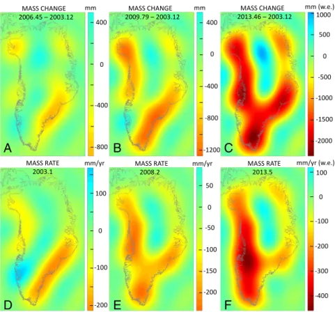
We address the spatial structure of the mass accelerations discussed above, by applying the same annual cycle plus quadratic trend model to each cell or“pixel” in our time series of GRACE mass grids. Having fit the composite mass trajectory model to each grid cell in Greenland, we can remove the mean annual cycle, just as we did in Fig. 1B, so as to isolate the decycled or seasonally adjusted cumulative mass changes from 2003.12 to 2006.45, 2009.79, or 2013.46 (Fig. 4A–C). The first two subplots (Fig. 4 A and B) are similar to those of Khan et al. (2) (see their figure 6A and B), depicting the spread of ice loss from southeast to northwest Greenland between 2003 and 2009. We also estimated the decycled mass rate as a function of time (Fig. 4D–F), by taking the first temporal derivative of the quadratic mass trend curve. Note the change in sign of mass rate in southwest Greenland between 2003 and 2013.5. In all six subplots of Fig. 4, there is little signal in the central portion of north Greenland, and there is a large segment of the eastern GrIS margin where mass loss and mass rate are much weaker than to the north or south.
The decycled mass acceleration field for the reference period (Fig. 5A) is found by taking the second temporal derivative of the
mass trend model. In the event that the mass time series in any given location does not actually have a constant acceleration, then our estimate can be interpreted as the mean acceleration in the time period of interest. The spatial pattern of the GRACE acceleration field is nearly consistent with GNET’s acceleration field (Fig. 2A andSI Appendix, Fig. S2A), once we take into account that the elastic responses to mass loss diminish with increasing distance from the centers of ice loss (9, 10, 12). The strongest acceleration in mass loss occurred in and near southwest Green-land (Fig. 5A, sector “sw”;SI Appendix, section 7). A distinct, smaller, and less intense center of negative mass acceleration is seen in the northeast (Fig. 5A, sector “ne”).
We can visualize the mass anomaly associated with the Pause by examining the difference between the projected mass trajectory model and the GRACE solution at epoch 2014.45 (Fig. 5B). Al-ternatively, we can average the mass anomalies in the interval 2013.79–2014.45 just as we did in Fig. 1D, but now as a function of position (SI Appendix, Fig. S10). The two approaches yield similar results. It is instructive to compare the mass anomaly field (Fig. 5B), which characterizes the expected mass loss that did not occur (due to the Pause), with the mass acceleration field (Fig. 5A) that characterizes mass changes during the previous decade. Apart from a change of sign, the spatial patterns are broadly similar. This strongly suggests that the shifting phase of the NAO (in summer) drove most of the sustained mass acceleration and its abrupt de-mise. We argue below that the spatial footprint of the sustained acceleration field also reveals the sensitivity of the ice sheet to at-mospheric warming, not just the spatial pattern of warming itself.
Even given the unavoidable spatial smoothing of any acceleration field inferred from GRACE, we can conclude that the most neg-ative mass accelerations in Greenland (Fig. 5A) occurred in the central west and southwest margins of the GrIS. Shifts in dynamic mass balance (DMB), that is, mass changes driven by changing rates of glacial discharge, at Jakobshavn Isbrae (JI), certainly con-tributed to the observed mass acceleration in the central west margin before 2006 (ref. 10; SI Appendix, section 7). However, further south, there are almost no major marine-terminating gla-ciers, so the acceleration field in the southwest margin was domi-nated by SMB, not DMB. This conclusion is supported by model results computed by the regional climate models MAR (15, 16) and
A
C
B
Fig. 2. Mean station accelerations in uplift for two overlapping 5-y time pe-riods. (A) Mean accelerations in the period that began in 2008.4, or when each GNET GPS station was established (if afterward), and ended in 2013.4. (B) The mean accelerations in the time interval 2010.4–2015.4. (C) Empirical cumulative distribution functions (CDFs) for the accelerations in each time period. U-Accel, vertical acceleration.
Fig. 3. The combined daily uplift anomalies for 46 GNET stations, and the traveling 25th, 50th, and 75th percentiles of this data cloud. The uplift anomaly is defined as the difference between the observed uplift and a trajectory model consisting of a quadratic trend and a four-term Fourier series fit to all data in a reference period ending in 2013.4. The median anomaly displaces sharply downward at 2013.4 and never returns to zero. NF, # fre-quencies; NP=2, quadratic trend; SLTM, standard linear trajectory model.
APPLIED
P
HYSICAL
RACMO2 (5). The temporal correlation between summertime SMB and the phase of the NAO is seen in Fig. 1F. We estimated the best linear trend in SMB predicted by MAR for the years 2004– 2012 (Fig. 5C). SMB expressed in water equivalent has units of millimeters per year, so SMB trend has units of millimeters per square year, that is, mass acceleration. The SMB trend field is broadly consistent with the mass acceleration field before 2013, given that the MAR output has much higher resolution (∼10 km) than GRACE (∼334 km). GRACE’s inevitable blurring of the SMB trend field both broadens the zone of negative mass accel-eration in southwest Greenland, and lowers its amplitude. The MAR SMB trend in the northeast GrIS is more pronounced than in adjacent areas, but this local feature is a little less pronounced, and slightly displaced, relative to GRACE’s secondary peak in mass acceleration (Fig. 5A, “ne”) suggesting that in this area changes in ice dynamics also played a role, as discussed later on. Note that both GRACE and MAR agree on near-zero or slightly positive mass accelerations in the east and southeast margins (Fig. 5A, “e” and“se”), respectively. MAR’s result for the southeast is associated with positive snowfall anomalies. GNET reveals a slightly more complex situation in which accelerations in uplift rates change sign from one major outlet glacier to the next (Fig. 2A andSI Appendix, Fig. S2A). GRACE tends to smooth out these alternating accel-erations in dynamic mass change and blends the result with the more subdued SMB trend due to increased snowfall accumulation. Topography Modulates the Impact of Atmospheric Warming The negative phase of the NAO in summertime enhances melting over much of Greenland, but especially in west Greenland (13, 14). The progressive, pre-2013 warming of west Greenland summers was not as spatially focused as the strongest negative mass accelerations (Fig. 5 A and C). The spatial distribution of ablation is largely controlled by the spatial distribution of air temperature and solar
radiation. The ice sheet’s sensitivity to surface warming is strongly influenced by surface elevation. If the surface warms from −1 to 3 °C, for example, then the impact of 4 °C warming is vastly greater than if the surface warms from−5 °C to −1 °C. This is why simple models of melting are often expressed in terms of seasonal sums of positive degree-day (17, 18). The amount of melting induced by a temperature increase is strongly dependent on initial surface temperature, and thus on latitude and elevation (SI Appendix, Fig. S11), as well as time of year. The influence that surface elevation has on melting and runoff is enhanced by a powerful positive feedback. The ice exposed in the ablation zone has lower albedo than snow surfaces, leading to greater absorption of solar radiation. Indeed, the largest source of melt energy in the ablation zone is absorbed solar energy, not the transfer of sensible heat from the air (19). Nevertheless, the primary control on the geometry of the ab-lation zone is air temperature, and, at a given time of year, near-surface temperature is largely controlled by latitude and elevation. In a given latitude zone, lower topographic gradients near the margins of the ice sheet lead to a wider ablation zone, thus acting as primary controls on the spatial extent of the albedo feedback.
Even if the southeast and southwest margins of the GrIS were exposed to similar positive temperature trends, the mass loss trend would be more pronounced at the southwest margin because it has a far greater area of low elevation ice surface per unit length of margin than does the southeast margin (Fig. 5D). Similarly, the low elevation and surface slopes prevailing at the northeast margin ensure that it incorporates a far greater area of low elevation ice surface than does a similarly sized segment of the northernmost margin of the ice sheet, or a similarly sized segment of the east margin (region “e” in Fig. 5A) where surface elevations >2 km loom over the nearby edges of the ice sheet. This helps us explain the localized center of sustained negative mass acceleration in the northeast (Fig. 5A, ne). The locally enhanced sensitivity of the
A
B
C
D
E
F
Fig. 4. (A–C) Cumulative mass loss since 2003.12, after the mean seasonal cycle is removed, in millimeters of water equivalent (w.e.), or kilograms per square meter. (D–F) Instantaneous mass rates implied by the quadratic trend model, that is, decycled mass rate, in millimeters per year of water equivalent.
northeast margin to atmospheric forcing, relative to immediately adjacent areas, was also apparent in the correlated 2010 melting day and uplift anomalies reported by Bevis et al. (8) (see their figure 5). Transient regional warming has less impact on higher portions of the GrIS surface than on lower portions. The high mountains that dam the ice sheet in central east Greenland ensure that there is very little low surface ice per unit distance along the general trend of this ice margin, in comparison with the adjacent margins to the north and south (Fig. 5D). This largely explains the near zero mean mass acceleration rates we inferred for east Greenland (Fig. 5A, area “e”). In summary, we suggest that both the geographical distribution of the progressive summertime warming before 2013, which was mostly focused in the west of Greenland, and the spatial struc-ture of ice sheet sensitivity to atmospheric forcing, which is dominated by ice sheet topography near its margins, jointly ex-plain most of the spatial pattern of SMB trend (Fig. 5C) and the mass acceleration field (Fig. 5A) sensed by GRACE before 2013. This interpretation is supported by the recent history of runoff within the Taseriaq basin of southwest Greenland (20). Atmospheric Forcing, SMB and DMB
Accelerations in total ice mass change are driven by changes in SMB and DMB. (Note that DMB= −D, where D is discharge, so total ice mass balance= SMB + DMB = SMB − D.) DMB changes are commonly driven by (i) changes in ocean circulation and temperature, and (ii) changes in the floating portion of the ice sheet and the mélange of icebergs and sea ice, which modulates their buttressing effect. Both changes affect calving rates and the velocity of outlet glaciers, and cause inland changes in ice thickness.
The secondary negative mass acceleration peak in northeast Greenland (Fig. 5A, “ne”) has already been associated with dynamic thinning in and near the outlet glaciers of the Northeast Greenland Ice Stream (12), but this does not rule out a role for atmospheric
forcing. The observation that the mass anomaly field (Fig. 5B) as-sociated with the Pause has its third largest center of mass gain in northeast Greenland, close to a center of accelerating mass loss in the previous decade, does suggest that this area was also affected by the shifting phase of the NAO (21). All three GNET stations close to the GrIS margin in northeast Greenland recorded accelerating uplift from their date of installation through 2012 (12), and they all recorded negative uplift anomalies after mid-2013 (SI Appendix, Fig. S6). This reversal occurred rather later than 2013.4–2013.5,
pre-sumably because summer arrives later in this region than it does in southern or central Greenland, and therefore the nondevelopment of a previously typical negative SMB season would not be evident until later in the year. The fact that a sustained acceleration fol-lowed by an abrupt deceleration is evident for northeast Greenland in both the GRACE and GNET time series suggests a connection to the NAO-driven changes identified in southwest Greenland. The MAR SMB trend field (Fig. 5C) does indicate greater mass loss acceleration in the northeast sector than in either adjacent sector of the ice margin, but this is not quite as pronounced as one might expect based on the GRACE results (Fig. 5A).
We suggest that sustained summertime warming before 2013 drove a shift in DMB, as well as SMB, in northeast Greenland. There are at least two possible mechanisms: (i) regional warming drove a reduction in the extent of the floating ice sheet before the summer of 2013, which diminished its buttressing effect on the outlet glaciers, prompting increased rates of discharge which thin-ned the ice, as observed in the Antarctic Peninsula (22, 23), and (ii) increases in meltwater production can modulate dynamical changes in ice mass. The northeast margin of the GrIS has a much greater area of low elevation surface than the margin sectors on either side (Fig. 5D), which would expand the area of enhanced meltwater production. Increased surface melting lowers the viscosity of the ice sheet via the advection of latent heat to its interior (24), and this
A
B
C
D
E
F
G
Fig. 5. (A) The seasonally adjusted mean mass ac-celeration field for the time period 2003.12–2013.46, in millimeters per square year of water equivalent. (B) The spatial structure of the“2013–2014 mass anomaly” defined as the mass residual field at epoch 2014.45. Note the negative correlation of A and B. (C) The temporal trend in SMB estimated using MAR during the years 2004–2012. The units, millimeters per square year, match those of subplot A. (D) Sur-face elevation of the GrIS. The 1,750-m above sea level (ASL) contour (black curve) was added to em-phasize lateral variability of the mean topographic slope near the ice margin, and changes in the margin-perpendicular width of the zones in which the ice surface lies below some reference height such as 500, 1,000, or 1,750 m ASL. (E) Precipitation, run-off, and SMB for Greenland as a whole, from MAR. (F) Greenland’s cumulative (CUM) SMB anomaly rel-ative to 1980–2002. (G) Cumulative runoff in south-west Greenland from MAR.
APPLIED
P
HYSICAL
mechanism will be volumetrically concentrated in thinner portions of ice sheet associated with low surface elevations. Meltwater can also accelerate ice flow by modifying the mechanical conditions at the base of the ice sheet (25–27). In extreme cases, the develop-ment of subglacial lakes can lift portions of an ice sheet or an ice cap from its bed (28, 29). The hypothesis that atmospheric warming can promote increases in discharge, dynamic thinning, and glacial retreat has recently been invoked in Prudhoe Land in northwest Greenland (30).
Discussion
The coverage and quality of our meteorological, glaciological, and geodetic datasets decline as we regress to the mid-1900s, as does our ability to track the relative importance of SMB and DMB as drivers of deglaciation. Even so, it is clear that the sustained acceleration in mass loss recorded by GRACE before mid-2013 was completely unprecedented (31), as was the collapse of seasonally adjusted mass rate from its peak value to nearly zero in the following 12–18 mo. Mass rate scales with SMB and DMB, so mass acceleration scales with the trend or rate of change of SMB and DMB. Greenland’s air–sea–ice system crossed one or more thresholds or tipping points near the beginning of this millennium, triggering more rapid de-glaciation. The pronounced negative shift in spatially integrated SMB (Fig. 5E andSI Appendix, Fig. S8) was dominated by increased summertime runoff (Fig. 5E and G). Runoff increased over most of the flanks of the GrIS, but most noticeably in southwest Greenland, where the margin was gaining mass in 2003 but strongly losing mass by late 2012 (Fig. 4). Total glacial discharge integrated over southwest Greenland is not only very low (9.5± 1.5 Gt/y) compared with other areas (32), it has been unusually stable as well. South of JI, mass acceleration was dominated by falling SMB from 2000 onward. A little further north, seasonally adjusted discharge rates at JI in-creased by ∼44% from early 2000 to early 2006, but barely changed between early 2006 and early 2012 (32). It was SMB that
was strongly falling in this second 6-y time interval, not DMB (10). Similar considerations apply in southeast Greenland (32).
The decadal acceleration in mass loss in southwest Greenland arose due to the combination of sustained global warming and positive fluctuations in temperature and insolation driven by the NAO. InSI Appendix, we develop an analogy with the global coral bleaching events triggered by every El Niño since that of 1997/1998, but not by any earlier El Niño event. Since 2000, the NAO has worked in concert with global warming to trigger major increases in summertime runoff. Before 2000, the air was too cool for the NAO to do the same. In a decade or two, global warming will be able to drive 2012 levels of runoff with little or no assistance from the NAO. In the shorter term, we can infer that the next time NAO turns strongly negative, SMB will trend strongly negative over west and especially southwest Greenland, just as future warming of the shallow ocean is expected to have its largest impact, via DMB (33, 34), in southeast and northwest Greenland. Because ice sheet to-pography equips southwest Greenland with greater sensitivity to atmospheric forcing, we infer that within two decades this part of the GrIS will become a major contributor to sea level rise. There is also the suggestion that enhanced summertime melting may induce more sustained increases in discharge rates.
Materials and Methods
We used the global GRACE solution CSR release RL-05. Our regional GRACE analysis used the methodology of ref. 3. Our GPS data processing followed that of ref. 6, as did our approach to time series analysis, both for GRACE and GNET. We characterized SMB in Greenland using the regional climate models MAR (15) and RACMO2 (5). Further details, and a discussion of data access, can be found inSI Appendix.
ACKNOWLEDGMENTS. We thank Robin Abbot of Polar Field Services for her unflagging logistical support. We are grateful to two anonymous reviewers for their comments and suggestions. This research and GNET were supported by National Science Foundation Grant PLR-1111882.
1. Velicogna I, Wahr J (2006) Acceleration of Greenland ice mass loss in spring 2004. Nature 443:329–331.
2. Khan SA, Wahr J, Bevis M, Velicogna I, Kendrick E (2010) Spread of ice mass loss into northwest Greenland observed by GRACE and GPS. Geophys Res Lett 37:L06501. 3. Harig C, Simons FJ (2012) Mapping Greenland’s mass loss in space and time. Proc Natl
Acad Sci USA 109:19934–19937.
4. Wouters B, et al. (2014) GRACE, time-varying gravity, Earth system dynamics and climate change. Rep Prog Phys 77:116801.
5. Van den Broeke MR, et al. (2016) On the recent contribution of the Greenland ice sheet to sea level change. Cryosphere 10:1933–1946.
6. Bevis M, Brown A (2014) Trajectory models and reference frames for crustal motion geodesy. J Geod 88:283–311.
7. Chen X, et al. (2017) The increasing rate of global mean sea-level rise during 1993– 2014. Nat Clim Change 7:492–495.
8. Bevis M, et al. (2012) Bedrock displacements on Greenland driven by ice mass varia-tions, climate cycles and climate change. Proc Natl Acad Sci USA 109:11944–11948. 9. Nielsen K, et al. (2012) Crustal uplift due to ice mass variability on Upernavik Isstrøm,
west Greenland. Earth Planet Sci Lett 353-354:182–189.
10. Nielsen K, et al. (2013) Vertical and horizontal surface displacements near Jakobshavn Isbrea driven by melt-induced and dynamic ice loss. J Geophys Res 118:1–8. 11. Khan SA, et al. (2016) Geodetic measurements reveal similarities between post-Last
Glacial Maximum and present-day mass loss from the Greenland ice sheet. Sci Adv 2: e1600931.
12. Khan A, et al. (2014) Sustained mass loss of the northeast Greenland ice sheet trig-gered by regional warming. Nat Clim Change 4:292–299.
13. Van Angelen J, et al. (2014) Contemporary (1960–2012) evolution of the climate and surface mass balance of the Greenland ice sheet. Surv Geophys 35:1155–1174. 14. Fettweis X, et al. (2013) Brief communication“Important role of the mid-tropospheric
atmospheric circulation in the recent surface melt increase over the Greenland ice sheet.” Cryosphere 7:241–248.
15. Fettweis X, et al. (2013) Estimating the Greenland ice sheet surface mass balance contribution to future sea level rise using the regional atmospheric climate model MAR. Cryosphere 7:469–489.
16. Fettweis X, et al. (2017) Reconstructions of the 1900–2015 Greenland ice sheet surface mass balance using the regional climate MAR model. Cryosphere 11:1015–1033. 17. Brathwaite R (1995) Positive degree-day factors for ablation on the Greenland ice
sheet studied by energy-balance modeling. J Glaciol 41:153–160.
18. Lecavalier B, et al. (2014) A model of Greenland ice sheet deglaciation constrained by observations of relative sea level and ice extent. Quat Sci Rev 102:54–84.
19. Van den Broeke MR, Smeets C, van de Wal R (2011) The seasonal cycle and in-terannual variability of surface energy balance and melt in the ablation zone of the west Greenland ice sheet. Cryosphere 5:377–390.
20. Ahlstrøm AP, Petersen D, Langen PL, Citterio M, Box JE (2017) Abrupt shift in the observed runoff from the southwestern Greenland ice sheet. Sci Adv 3:e1701169. 21. Tedesco M, et al. (2016) Arctic cut-off high drives the poleward shift of a new
Greenland melting record. Nat Commun 7:11723.
22. Wendt J, et al. (2010) Recent ice-surface-elevation changes of Fleming Glacier in re-sponse to the removal of the Wordie Ice Shelf, Antarctic Peninsula. Ann Glaciol 51: 97–102.
23. Rott H, Müller F, Nagler T, Floricioiu D (2011) The imbalance of glaciers after dis-integration of Larsen-B ice shelf, Antarctic Peninsula. Cryosphere 5:125–134. 24. Phillips T, Rajaram H, Colgan W, Steffen K, Abdalati W (2013) Evaluation of
cryo-hydrologic warming as an explanation for increased ice velocities in the wet snow zone, Sermeq Avannarleg, West Greenland. J Geophys Res 188:1241–1256. 25. Parizek BR, Alley RB (2004) Implications of increased Greenland surface melt under
global-warming scenarios: Ice-sheet simulations. Quat Sci Rev 23:1013–1027. 26. Schoof C (2010) Ice-sheet acceleration driven by melt supply variability. Nature 468:
803–806.
27. Bartholomew I, et al. (2012) Short-term variability in Greenland ice sheet motion forced by time-varying meltwater drainage: Implications for the relationship between subglacial drainage system behavior and ice velocity. J Geophys Res 117:F03002. 28. Das SB, et al. (2008) Fracture propagation to the base of the Greenland ice sheet
during supraglacial lake drainage. Science 320:778–781.
29. Willis MJ, Herried BG, Bevis MG, Bell RE (2015) Recharge of a subglacial lake by sur-face meltwater in northeast Greenland. Nature 518:223–227.
30. Sakakibara D, Sugiyama S (2018) Ice front and flow speed variations of marine-terminating outlet glaciers along the coast of Prudhoe Land, northwestern Green-land. J Glaciol 64:300–310.
31. Khan SA, et al. (2015) Greenland ice sheet mass balance: A review. Rep Prog Phys 78: 046801.
32. King M, et al. (2018) Seasonal to decadal variability in ice discharge from the Greenland ice sheet. Cryosphere 12:3813–3825.
33. Holland D, Thomas R, De Young B, Ribergaard M, Lyberth B (2008) Acceleration of Jakobshavn Isbrae triggered by warm subsurface ocean waters. Nat Geosci 1:659–664. 34. Straneo F, Heimbach P (2013) North Atlantic warming and the retreat of Greenland’s