Université de Montréal
Modelling Software Quality: A Multidimensional Approach
par
Stéphane Vaucher
Département d’informatique et de recherche opérationnelle Faculté des arts et des sciences
Thèse présentée à la Faculté des arts et des sciences en vue de l’obtention du grade de Philosophiæ Doctor (Ph.D.)
en informatique
Août, 2010
c
Université de Montréal Faculté des arts et des sciences
Cette thèse intitulée:
Modelling Software Quality: A Multidimensional Approach
présentée par: Stéphane Vaucher
a été évaluée par un jury composé des personnes suivantes: Jian-Yun Nie, président-rapporteur Houari Sahraoui, directeur de recherche Bruno Dufour, membre du jury Massimiliano Di Penta, examinateur externe Khalid Benabdallah, représentant du doyen de la F.A.S.
RÉSUMÉ
Les sociétés modernes dépendent de plus en plus sur les systèmes informatiques et ainsi, il y a de plus en plus de pression sur les équipes de développement pour produire des logiciels de bonne qualité. Plusieurs compagnies utilisent des modèles de qualité, des suites de programmes qui analysent et évaluent la qualité d’autres programmes, mais la construction de modèles de qualité est difficile parce qu’il existe plusieurs questions qui n’ont pas été répondues dans la littérature. Nous avons étudié les pratiques de modélisa-tion de la qualité auprès d’une grande entreprise et avons identifié les trois dimensions où une recherche additionnelle est désirable : Le support de la subjectivité de la qua-lité, les techniques pour faire le suivi de la qualité lors de l’évolution des logiciels, et la composition de la qualité entre différents niveaux d’abstraction.
Concernant la subjectivité, nous avons proposé l’utilisation de modèles bayésiens parce qu’ils sont capables de traiter des données ambiguës. Nous avons appliqué nos modèles au problème de la détection des défauts de conception. Dans une étude de deux logiciels libres, nous avons trouvé que notre approche est supérieure aux techniques décrites dans l’état de l’art, qui sont basées sur des règles.
Pour supporter l’évolution des logiciels, nous avons considéré que les scores produits par un modèle de qualité sont des signaux qui peuvent être analysés en utilisant des techniques d’exploration de données pour identifier des patrons d’évolution de la qualité. Nous avons étudié comment les défauts de conception apparaissent et disparaissent des logiciels.
Un logiciel est typiquement conçu comme une hiérarchie de composants, mais les modèles de qualité ne tiennent pas compte de cette organisation. Dans la dernière partie de la dissertation, nous présentons un modèle de qualité à deux niveaux. Ces modèles ont trois parties : un modèle au niveau du composant, un modèle qui évalue l’importance de chacun des composants, et un autre qui évalue la qualité d’un composé en combinant la qualité de ses composants. L’approche a été testée sur la prédiction de classes à fort changement à partir de la qualité des méthodes. Nous avons trouvé que nos modèles à deux niveaux permettent une meilleure identification des classes à fort changement.
Pour terminer, nous avons appliqué nos modèles à deux niveaux pour l’évaluation de la navigabilité des sites web à partir de la qualité des pages. Nos modèles étaient capables de distinguer entre des sites de très bonne qualité et des sites choisis aléatoirement.
Au cours de la dissertation, nous présentons non seulement des problèmes théoriques et leurs solutions, mais nous avons également mené des expériences pour démontrer les avantages et les limitations de nos solutions. Nos résultats indiquent qu’on peut espérer améliorer l’état de l’art dans les trois dimensions présentées. En particulier, notre travail sur la composition de la qualité et la modélisation de l’importance est le premier à cibler ce problème. Nous croyons que nos modèles à deux niveaux sont un point de départ intéressant pour des travaux de recherche plus approfondis.
Mots clés: Génie logiciel, qualité du logiciel, modèles de qualité, études empi-riques, réseaux bayésiens, évolution du logiciel, composition de la qualité.
ABSTRACT
As society becomes ever more dependent on computer systems, there is more and more pressure on development teams to produce high-quality software. Many com-panies therefore rely on quality models, program suites that analyse and evaluate the quality of other programs, but building good quality models is hard as there are many questions concerning quality modelling that have yet to be adequately addressed in the literature. We analysed quality modelling practices in a large organisation and identi-fied three dimensions where research is needed: proper support of the subjective notion of quality, techniques to track the quality of evolving software, and the composition of quality judgments from different abstraction levels.
To tackle subjectivity, we propose using Bayesian models as these can deal with uncertain data. We applied our models to the problem of anti-pattern detection. In a study of two open-source systems, we found that our approach was superior to state of the art rule-based techniques.
To support software evolution, we consider scores produced by quality models as signals and the use of signal data-mining techniques to identify patterns in the evolution of quality. We studied how anti-patterns are introduced and removed from systems.
Software is typically written using a hierarchy of components, yet quality models do not explicitly consider this hierarchy. As the last part of our dissertation, we present two level quality models. These are composed of three parts: a component-level model, a second model to evaluate the importance of each component, and a container-level model to combine the contribution of components with container attributes. This approach was tested on the prediction of class-level changes based on the quality and importance of its components: methods. It was shown to be more useful than single-level, traditional approaches.
To finish, we reapplied this two-level methodology to the problem of assessing web site navigability. Our models could successfully distinguish award-winning sites from average sites picked at random.
but we performed experiments to illustrate the pros and cons of our solutions. Our results show that there are considerable improvements to be had in all three proposed dimensions. In particular, our work on quality composition and importance modelling is the first that focuses on this particular problem. We believe that our general two-level models are only a starting point for more in-depth research.
Keywords: Software engineering, software quality, quality models, empirical studies, Bayesian models, software evolution, quality composition.
CONTENTS
RÉSUMÉ . . . . v
ABSTRACT . . . vii
CONTENTS . . . ix
LIST OF TABLES . . . xv
LIST OF FIGURES . . . xvii
LIST OF APPENDICES . . . xix
ACKNOWLEDGMENTS . . . xxi CHAPTER 1: INTRODUCTION . . . . 1 1.1 A Historical Perspective . . . 1 1.2 Defining Quality . . . 3 1.3 Ensuring Quality . . . 5 1.4 Problem Statement . . . 7
1.4.1 Manipulation of Higher-order Concepts . . . 7
1.4.2 Tracking the Evolution of Quality . . . 8
1.4.3 Quality Composition . . . 8
1.5 Dissertation Organisation . . . 8
CHAPTER 2: BACKGROUND . . . 11
2.1 Quality Models . . . 11
2.1.1 Definitional Models . . . 11
2.1.2 Operational Quality Models . . . 13
2.2 Model Building . . . 15
2.2.2 What can we Measure? . . . 16
2.2.3 Quality Indicators . . . 17
2.2.4 Notable Code Metrics . . . 19
2.3 Model Building Techniques . . . 21
2.3.1 Regression Techniques . . . 21
2.3.2 Machine-Learning Techniques . . . 23
2.4 Open Issues in Quality Modelling . . . 25
2.4.1 Incompatibility of Measurement Tools . . . 25
2.4.2 Unwieldy Distributions . . . 26
2.4.3 Validity of Metrics . . . 27
2.4.4 The Search for Causality . . . 28
2.5 Conclusion . . . 29
CHAPTER 3: STATE OF PRACTICE IN QUALITY MODELLING . . . 31
3.1 Quality Modelling Practices: an Industrial Case Study . . . 31
3.1.1 Quality Evaluation Process . . . 33
3.1.2 Issues . . . 35
3.2 Initial Exploration of Concerns . . . 37
3.2.1 Systems Studied . . . 38
3.2.2 Metrics Studied . . . 39
3.2.3 Analysis Techniques . . . 40
3.2.4 Issue 1: Usefulness of Metrics . . . 40
3.2.5 Issue 2: Combination Strategies . . . 41
3.3 Research Perspectives . . . 44
3.4 Conclusion . . . 45
CHAPTER 4: DEALING WITH SUBJECTIVITY . . . 47
4.1 Existing Techniques to Model Subjectivity . . . 48
4.1.1 Fuzzy Logic . . . 48
4.1.2 Bayesian Inference . . . 50
xi
4.2.1 Industrial Interest in Anti-pattern Detection . . . 51
4.2.2 The Subjective Nature of Pattern Detection . . . 54
4.2.3 Detection Methodology . . . 54
4.2.4 Evaluating our Bayesian Methodology . . . 58
4.2.5 Scenario 1: General Detection Model . . . 61
4.2.6 Scenario 2: Locally Calibrated Model . . . 64
4.3 Discussion of the Results . . . 66
4.3.1 Threats to Validity . . . 66
4.3.2 Dealing with Good Programs . . . 66
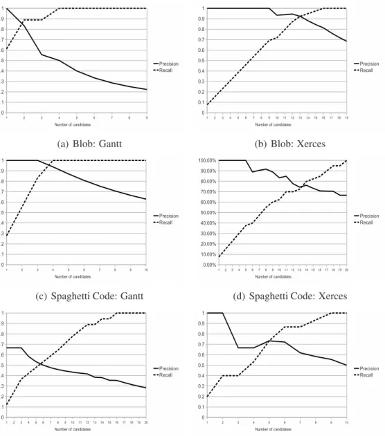
4.3.3 Estimating the Number of Anti-Patterns . . . 67
4.3.4 Alternative Code Representation . . . 68
4.4 Conclusion . . . 68
CHAPTER 5: ANALYSING THE EVOLUTION OF QUALITY . . . 69
5.1 Industrial Practice . . . 69
5.2 State of the Research . . . 70
5.3 Identifying and Tracking Quality . . . 72
5.3.1 Dealing with Temporal Data . . . 72
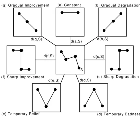
5.3.2 Quality Trend Analysis . . . 73
5.3.3 Finding Quality Trends . . . 74
5.4 Tracking Design Problems . . . 74
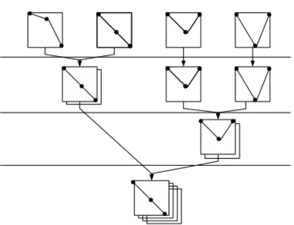
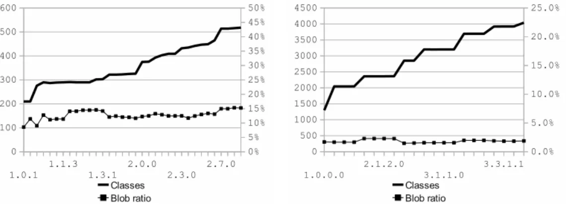
5.4.1 Global View on the Evolution of Blobs . . . 75
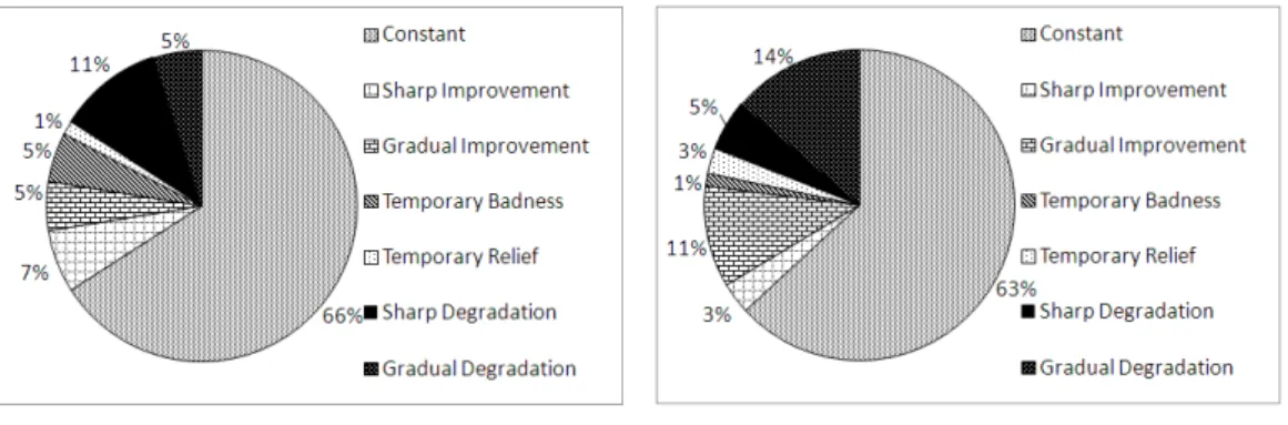
5.4.2 Evolution Trends Identified . . . 76
5.5 Discussion . . . 81
5.5.1 How to Track Blobs? . . . 82
5.5.2 How to Remove Blobs? . . . 82
5.6 Conclusion . . . 83
CHAPTER 6: HIERARCHICAL MODELS FOR QUALITY AGGREGA-TION . . . 85
6.2 Modelling Code Changeability . . . 88
6.2.1 Change Models . . . 89
6.2.2 Determining Method Importance . . . 92
6.3 Comparing Aggregation Strategies . . . 99
6.3.1 Study Definition and Design . . . 99
6.3.2 Data Analysed . . . 99
6.3.3 Variables Studied . . . 101
6.3.4 Operationalising the Change Models . . . 102
6.3.5 Results . . . 105
6.3.6 Discussion . . . 110
6.4 Related Work . . . 113
6.5 Conclusion . . . 115
CHAPTER 7: COMPOSITION OF QUALITY FOR WEB SITES . . . . 117
7.1 Problem Statement . . . 117
7.1.1 Finding Information on a Web Site . . . 118
7.1.2 Assessing Site Navigability . . . 119
7.2 Related Work . . . 120
7.3 A Multi-level Model to Assess Web Site Navigability . . . 121
7.3.1 Bayesian Belief Networks . . . 121
7.3.2 Assessing a Web Page . . . 122
7.3.3 Navigation Model . . . 126
7.3.4 Assessing a Web Site . . . 128
7.4 Case Study . . . 129
7.4.1 Study Setup . . . 129
7.4.2 Navigability Evaluation Results . . . 130
7.4.3 Discussion . . . 130
7.5 Conclusion . . . 133
CHAPTER 8: CONCLUSION . . . 135
xiii
8.1.1 Handling Subjectivity . . . 136
8.1.2 Supporting Evolution . . . 137
8.1.3 Composing Quality Judgements . . . 138
8.1.4 Application to Web Applications . . . 138
8.2 Future Research Avenues . . . 139
8.2.1 Crowd-sourcing . . . 139
8.2.2 Using Complex Structures instead of Metrics . . . 139
8.2.3 Activity Modelling . . . 141
8.3 Other Research Paths Explored . . . 141
8.4 Closing Words . . . 144
LIST OF TABLES
3.I Method-level metrics studied . . . 39
3.II Class-level metrics studied . . . 39
3.III Descriptive statistics for the NASA data set . . . 40
3.IV Rank correlations between method metrics and bug count . . . 41
3.V Rank correlations between class metrics and bug count . . . 42
3.VI Classification rates for class fault-proneness . . . 43
4.I GQM applied to Blobs . . . 55
4.II GQM applied to Spaghetti Code . . . 55
4.III GQM applied to Functional Decomposition . . . 56
4.IV Program Statistics . . . 59
4.V Salient symptom identification . . . 60
4.VI JHotDraw: inspection sizes . . . 67
5.I Degradation growth rates in Xerces . . . 80
5.II Refactorings identified in Xerces for the correction of Blobs . . . 81
6.I Relative weights for each importance function. . . 98
6.II Descriptive statistics for replication data . . . 100
6.III Correlations: number of changes and class metrics/model output 106 6.IV Correlations: number of changes and scores (type 2 models) . . . 107
6.V Correlations: number of changes and scores (type 3 models) . . . 109
7.I Inputs to the navigability model . . . 124
7.II Page navigability CPT . . . 126
LIST OF FIGURES
2.1 ISO9126 quality decomposition . . . 12
2.2 Distribution of cyclomatic complexity . . . 26
3.1 Fault distribution per development phase . . . 32
3.2 Stakeholders in a quality evaluation process . . . 32
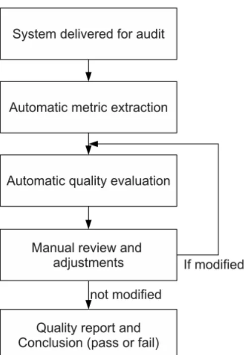
3.3 Quality evaluation process of our partner . . . 34
3.4 Example of industrial quality models . . . 34
3.5 Example of a maintainability model . . . 35
3.6 Fault-proneness model using method-level metrics . . . 44
3.7 Fault-proneness model using class-level metrics . . . 44
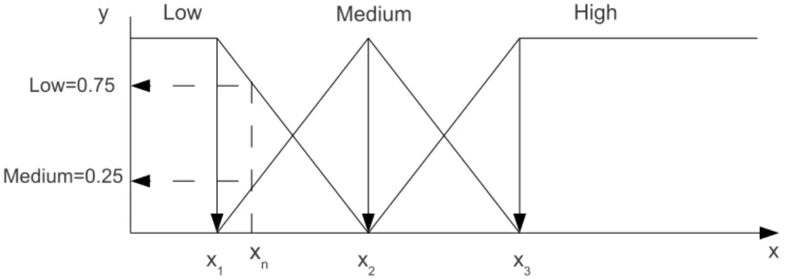
4.1 Fuzzification process of a metric value . . . 49
4.2 Functional decomposition detection rules . . . 52
4.3 GQM applied to the Blob . . . 56
4.4 Probability interpolation for metrics . . . 57
4.5 Inspection process for Bayesian inference . . . 62
4.6 Inter-project validation . . . 63
4.7 Local calibration: average precision and recall . . . 65
5.1 Quality signal . . . 73
5.2 Dendrogram of quality signals . . . 75
5.3 Blob Ratios vs. Total Classes . . . 76
5.4 Evolution Trend Classification . . . 77
5.5 Evolution Trends Distribution of Blobs . . . 78
6.1 Logical decomposition of a system . . . 86
6.2 General composition model . . . 87
6.3 Class-method composition model . . . 88
6.4 Single-level change model . . . 90
6.6 Sample method-level model . . . 91
6.7 Modified type 1 change model to support method-level quality models . . . 91
6.8 Aggregation models for method-level evaluations . . . 92
6.9 Simple call graph between methods in their classes . . . 95
6.10 Simple call graph between methods in their classes . . . 98
6.11 Method change model . . . 103
6.12 Inspection efficiency for different sized inspections using class-level information . . . 107
6.13 Inspection efficiency for different standard aggregation strategies . 108 6.14 Inspection efficiency for different sized inspections by combining method-level information . . . 110
6.15 Inspection efficiency (in terms of size) . . . 111
7.1 Navigability Evaluation Process . . . 119
7.2 The original page-level navigability model: site-level metrics are identified in light gray . . . 123
7.3 The modified page-level navigability model . . . 123
7.4 Binary input classification . . . 125
7.5 Site-level quality model . . . 129
7.6 Navigability scores for good and random sites . . . 131
7.7 Initial model . . . 132
LIST OF APPENDICES
ACKNOWLEDGMENTS
I thank my advisor, Houari Sahraoui for introducing me to the problems with empir-ical software engineering. He taught me that good experimentation is difficult and needs to be done in a rigorous manner. He also helped me become independent by assisting in the supervision of other students in my research group.
I would like to thank my collaborators. I thank Foutse Khomh who was a great research partner, for our great discussions that lead to multiple publications. I thank Prof. Yann-Gaël Guéhéneuc for his great toolkit (Ptidej), scientific discussions, and moral support. I also thank Marouane Kessentini and Prof. Naouel Moha, for our productive partnerships concerning anti-patterns. Finally, I would like to thank Simon Allier and Prof. Bruno Dufour for their help understanding how call graphs work.
Most importantly, my Ph.D. would not have been possible without the support of my wife, my “grande pitoune”, Catherine and the love of my two-year-old “petite pitoune”, Fiona. I would also thank my pop, Jean Vaucher, for his help focusing my ideas and for rereading my dissertation.
CHAPTER 1 INTRODUCTION
At the start of the 21st century, software is at the heart of many important aspects of society. Not only are these software systems omnipresent, but their complexity is an order of magnitude greater than anything produced ten years ago. These systems were built over the course of many years during which developers come and leave. The consequence is that keeping an old system up to date with new requirements is very expensive. Conservative studies show that well over 50% of effort is spent on mainte-nance [Bel00, HM00]. In this context, it is important to have tools and techniques to regularly check the quality of these systems to ensure that, with time, a system does not become a burden.
1.1 A Historical Perspective
In the sixties, IBM decided to advance the state of the art with an ambitious operat-ing system called OS/360. At the time, this OS was one of the most complex software ever undertaken. Although eventually a commercial success, its development proved to be almost too difficult to manage, going billions over budget: the estimate was 675 million dollars, but it cost 5 billion dollars [IBM08]. At its peak, over 50,000 em-ployees were working on the project. The cost of the project was such that it was famously coined the 5 billion dollar gamble by Fortune magazine, for if the project failed, IBM would have gone bankrupt. Many important lessons were learned from this ordeal [FPB78], and these contributed to the emergence of the field of software engi-neering as its managerial failure was much discussed in the NATO Software engiengi-neering conferences [NR69, BR70].
The NATO conferences had the objective of shaping the field of software engineer-ing. It was for this purpose that different participants described issues with producing good software. One of the most important issues raised was how to scale production up
to the new large systems and limit costs. The main method was to improve the process of “manufacturing code”. They argued that process improvement would improve software
quality, a term mostly reserved to describe software that conforms to its specification
and that contains few bugs. The advantage of having “clean” code was expressed only once, by M.D. McIlroy (p.53 [NR69]). He stated that some effort should be spent to evaluate the “quality of work” of a programmer, by assessing its readability.
Since the early days of software engineering, the notion of quality has had to evolve. It was typically thought that a system would be developed, and as soon as all the bugs were found and corrected, it would then be used with little or no modification. Even-tually, the system would be retired and replaced by a newer system. This was not the case. The construction of these early monster systems was not cost-efficient, and there-fore management moved towards an evolution model hoping to reuse previously coded artefacts. In this context, the seemingly unimportant factor of readability becomes very important. The predominant methodologies like the waterfall model [Roy70] focused on the production of a final, functional system; these were not adapted to the reality of modifying large-scale systems [McC04].
Another important change to software systems is their increasing level of interactiv-ity. In the sixties and seventies, programs were batch-oriented and there was little to no interaction. Ever since the advent of user interfaces, user expectations in terms of usability have constantly increased. Currently, trends on the Web even allow users to interact with each other with user-generated content. Consequently, for modern soft-ware to be successful, it should not only provide bug-free functionality, but it should do so with an adequate user-experience. Concerning the issues of user perceived quality, Kan [Kan95] states that it is an ambiguous, multi-dimensional concept. In particular, he distinguishes between the user view of quality which can be experienced but not defined, and the professional view which can be measured and controlled. Of course, the view of professionals is difficult to assess objectively because it is determined by their specific quality-related needs.
3 1.2 Defining Quality
According to the Oxford Dictionary, quality is the degree of excellence of a thing. A quality software system is one that works well and gives satisfaction. With the majority of effort being spent to maintain systems [Bel00, HM00], we can assume that quality should mean that the system will continue to give satisfaction in the future.
For a broader understanding of software quality, Kitchenham and Phleeger [KP96] refer to the work of David Garvin [Gar84]. Garvin presents case studies of quality management from different industries, mostly manufacturing. He reports five views of quality:
• The transcendental view: quality can be recognized, but not defined. This can be seen as the idealised view of quality presented by software evangelists;
• The user view: quality is how well a product suits a user’s needs. This view considers, but is not limited to, the notion of crashes as it relates to user experience; • The manufacturing view: quality can be guaranteed by following a well-controlled series of steps. This perspective focuses on improving the development process. It follows the philosophy that by following a good process, we should be able to produce good software;
• The product view: the quality of software depends on its internal characteristics. This is the view of most metrics advocates. If a product is well written, then an external perception of quality should in turn be good;
• The value view: quality depends on what someone would pay for it. This is typi-cally a viewpoint of investors and upper management.
Each of these views corresponds to that of different types of stakeholders. Ideally, the best product would satisfy all these stakeholders, but this is rarely the case. For example, a development team might consider their code base unwieldy and would like to restructure (product view), but management does not want to spend more on the product as the restructuring might not produce enough value (value view) [BAB+05].
Kitchenham and Phleeger then used these views to organise the results of a survey. The majority of respondents said that the manufacturing and user views were the most important. Ironically, other research suggests that users often do not know what they would like unless they experience it first [Gla09]. Without this experience, users will focus on an idealised view of what they want (e.g. multitude of features and few bugs). However, his idealised view rarely corresponds to their actual appreciation of the sys-tem [Sch03b].
It is impossible to find a universally accepted notion of quality as it depends both on the application domain and on the needs of the different stakeholders. For example, the aeronautics industry needs for their systems to be as reliable as possible by avoiding failures. A text editor would obviously not have the same reliability requirement; instead, it might have a requirement to be user-friendly. The perception of quality also depends very much on the stakeholder. Managers might be interested in limiting the cost of maintaining old systems while a user would have other criteria to evaluate quality.
The abstract nature of quality is a problem as quality control is an important part of all fields of engineering. In software engineering, we therefore use concrete, useful approximations of quality (e.g., absence of bugs) and try to exploit this data to improve the quality of software to enable various stakeholders to make enlightened decisions. For example, we might like to know when a system is reliable enough to be released.
The objective of quality modelling is to describe relationships between different ex-plicative factors and quality. Until now, we have focused on quality as an abstract con-cept. However, for it to be understood and controlled, it first needs to be measured, and the exact measurement to hard to define. Furthermore, this measure can be difficult to collect because it cannot be measured directly on the system. Rather, it is observed in a specific context that is domain and stakeholder dependent. For example, to measure reliability, it is possible to use the average up time of a system. This measure would obviously require the system to be executed.
5 1.3 Ensuring Quality
There are many approaches proposed to produce and ensure high-quality software. One approach considers the process used to build software. By setting up a process that includes quality-assurance activities, the perceived quality of a system should increase. In fact, over the past decades, there have been significant process-level improvements which in turn have improved the software produced. There are many existing method-ologies that focus on different perceptions of quality. For example, the Cleanroom pro-cess [MDL87] is focused on defect prevention. On the other hand, agile methodologies like eXtreme programming [Bec99] try to keep software as flexible as possible in order to quickly get feedback from its users.
To ensure quality, these development methodologies rely on activities like formal methods, testing, and code inspections to judge if a system is ready to be released.
Formal methods use proofs to show that code actually conforms to a specification.
Formal methods are very expensive because they require well-defined specifications, and consequently are usually only used for important parts of mission critical applica-tions [Men08].
Testingis generally considered the most important quality assurance activity. It
con-sists of comparing the state and behaviour of a system to expectations; it can focus on different aspects like reliability, performance, and conformity to specification. However, it is limited to finding given specific parameters (e.g.finding faults within a specific exe-cution context). It therefore cannot guarantee the absence of problems. From a manage-ment standpoint, it is difficult to assess when enough testing has been completed before releasing software [oST02]. Testing is a relatively costly task: studies show that testing accounts for over 30% of forward development costs [Bei90], and many mission-critical systems even have more testing code than actual system code. Therefore, the amount of testing done is typically limited by the resources available. Testing can ensure that there are few bugs in a system and that the specification is followed, but it cannot predict future problems like high maintenance costs.
evaluate its quality. Code inspections are very useful as they can uncover a great variety of problems, some are functional [BS87, SBB+02], but many are concerned with abstract
notions of software quality like its capacity to be changed for future needs [ML08]. The basic idea is that well written code is good quality code, which needs minimal testing and which should be easy to maintain. Typically, inspectors will evaluate different as-pects of the code, like its understandability, the presence undue complexity, and the use of known robust patterns. This notion of quality is difficult to test as it depends not only on the satisfaction of current needs, but of future needs as well. To benefit from in-spections, developers need to read, understand, and comment code, which requires time. Consequently, this approach cannot be applied to the totality of a large system.
The idea motivating quality modeling is that code inspections are good, but require human intervention and are, therefore, too costly to be applied on the totality of a system. A quality model tries to automate the inspection process. As inputs, the model uses metrics which describe characteristics a human inspector would use, and tries to predict an inspector’s quality assessment. There are limits to what a model can do automatically. Although it tries to mimic an expert’s judgment, it can only analyse the surface structure of the system. For example, it can check for the presence of comments, check formatting, and even consider the size and links between different modules, but it cannot analyse elements of good design like meaningful comments, reuse of tested architectures and algorithms. A model may try to simulate a human process by using AI techniques.
Quality models can find different niches in different development processes. In agile development processes, they can be included in a continuous integration pro-cess [DMG07], and executed every day, informing developer of potential problems. In a more process-heavy methodology, these can be used by independent validation and verification teams who perform quality audits [MGF07].
As a quality model can evaluate the totality of a system, it can be used for two purposes. First, it can guide testing efforts and more elaborate inspections to certain parts of a system exhibiting bad properties. Second, knowing the quality of the different parts of a system, a model could provide an aggregate measure of the system. From a management perspective, a model can thus be used to guide decisions. They can,
7 for example, enforce quality-level obligations or estimate the cost of ownership of their systems.
1.4 Problem Statement
The current state of research focuses on proposing models that directly mimic a hu-man inspection process. Models typically use metrics describing structural properties (like size, coupling, and cohesion) of the system extracted either from design artefacts or directly from the source code. As outputs, they produce an estimated value of an indi-cator of quality like bugs or effort [LH93b, MK92, BBM96, HKAH96, KM90, OW02, NBZ06]. These two quality indicators are arguably the most unambiguous measures of quality as few can deny that a system that crashes should be fixed, or that a system that is expensive to maintain might need to be restructured.
There are however some problems with the application of state of the art techniques. At the start of our research, a large company asked us to evaluate their quality modeling efforts. They had performed a literature review and applied existing standards to build quality models. They wanted independent and knowledgeable experts to audit their ap-proach and suggest improvements. Our investigations of their modeling efforts identified the following problems in current research on quality modeling.
1.4.1 Manipulation of Higher-order Concepts
The first problem comes from the theory that underpins traditional fault-prediction models: that good design leads to good quality. The problem is that it is not obvious what good design is. Current practices rely on code-level metrics to decide if a module is well designed. Such approaches ignore the fact that good design conveys meaning and semantics that are not easily measurable. Therefore, we need to manipulate higher-order concepts (e.g., design patterns and practices), to improve the state of quality modelling. Unfortunately, there are no exact techniques to identify these semantically rich concepts. Furthermore, these concepts are useful only if they are applied to specific contexts. For example, a design pattern is a reusable solution for a specific type of problem.
Unfortu-nately, different developers might disagree on whether pattern is appropriate for a given context; this is because judging the quality of design is a subjective activity.
1.4.2 Tracking the Evolution of Quality
Good design allows developers to modify and improve a system. Recent research has included aspects of this when modelling quality. Typically, this is done by including changes in a quality model [MPS08, NB05b]. Yet, changes, like design, have strong semantic meanings. For example, changes can be done to add functionality or to correct a bug. There also exists work that tries to classify changes [AAD+08, MV00], but what
is lacking are techniques to identify changes in code that have a significant impact on the quality of a system.
1.4.3 Quality Composition
A final problem concerns the absence of quality composition models. Typically, a quality model evaluates quality on one specific type of software artefact, more often than not, the level for which we have access to quality indicators. In procedural code, the evaluated artefacts are either files or procedures; in object-oriented systems, the fo-cus is generally on classes. The quality of a system is a function of the quality of its constituents [BD02], but to the best of our knowledge, no research seeks to determine which types of aggregation functions are appropriate. For a decision-maker who wants a bird-eyes view of the state of their systems, the lack of a proper aggregation mechanism is a serious problem. For example, our partner uses an aggregated quality score to moni-tor outsourced maintenance activities. This score is then used to accept or reject changes to the system. They consequently need for this score to represent the actual quality of the system.
1.5 Dissertation Organisation
9 1. Chapter 2 covers quality models. It describes input variables, output variables and
model building techniques. It also describes open issues in quality modelling. 2. Chapter 3 covers industrial practice. We examined the practices at a large
com-pany and observed problems that influenced the directions of our research. We reproduced some of the issues raised on available data sets.
3. Chapter 4, addresses subjectivity in quality assessment. We proposed the use Bayesian models to support subjectivity. We successfully applied these models to the problem of anti-pattern detection.
4. Chapter 5 explains how to use quality models to track quality over time. We presented a signal analysis technique to identify quality change patterns.
5. Chapter 6, we present issues with quality composition, and propose a general model to enhance quality models to support composition relationships. We in-troduced the complex notion of importance when combining low-level data. Ex-perimentally, we show that our enhanced models can produce superior results to traditional single-level models.
6. Chapter 7 shows how our composition techniques can be applied to a different domain (web sites vs. executable code). In a study of 40 web sites, we found that our models could correctly distinguish good site from randomly selected ones. 7. We conclude the dissertation in Chapter 8, where we describe the lessons we
CHAPTER 2 BACKGROUND
This chapter presents the background material required to understand the evaluation of quality in software systems. In particular, we focus on quality models, and software metrics. We also provide an overview of existing techniques to build these models. Finally, we raise open issues pertaining to quality. Specific related work required to understand a specific chapter will be present at that moment.
2.1 Quality Models
The goal of modelling quality is to establish a relationship between measurable as-pects of a system and its quality. There are two types of quality models: definitional models and operational models. Definitional models decompose a high-level, abstract notion of quality into more concrete contributing factors. Operational models are some-times based on these definitional models, but the main difference is that they can be implemented and executed to produce quality scores.
2.1.1 Definitional Models
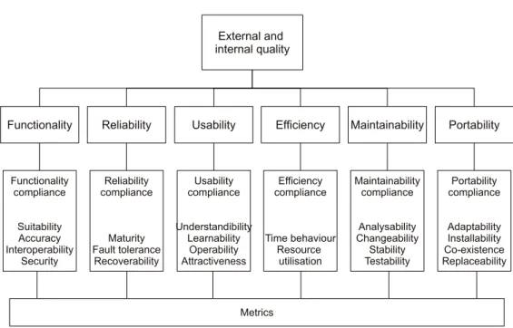
Many definitional models have been proposed: the McCall [MRW77], Boehm [Boe78], FURPS [GC87] and ISO 9126 [ISO91] models, to name a few. The first three models were created in specific industrial contexts while the last is an ISO standard. All models organise quality in a tree-like structure where quality character-istics are either measured directly or composed using other charactercharacter-istics (or subchar-acteristics). Figure 2.1 presents this progressive decomposition of quality into metrics. These models are interesting because they point out different non-functional aspects of software to consider when evaluating quality.
The first criticism of these models is that they are not operational. While they express the need for measurement, they do not define which exact metrics to use and how to
Figure 2.1: ISO9126 quality decomposition
combine information from one level to another. For example, the McCall and FURPS models consist of checklists of concepts to evaluate, but do not specify what to measure and how to obtain quality values [AKCK05]. Second, these standards are not based on empirically observed relationships, but rather on qualitative, sometimes anecdotal evidence [PFP94, JKC04]. Other criticism comes from the fact that these models have a limited view of quality which is based on a developer perspective instead of a managerial, more value-based perspective [Pfl01, BAB+05].
Another family of models is the result of the Dromey model [Dro95] building frame-work. The idea proposed is that abstract quality attributes cannot be measured directly. There are however quality-carrying properties that can be measured on the entities used to build the system. These properties can impact the abstract quality characteristics. Good properties should therefore be built into software to insure its good quality while bad properties should be avoided. As this is a model building framework, Dromey does not present how to implement and validate a model.
13 2.1.2 Operational Quality Models
The step between having a theoretical model and putting one into operation is com-plex. The literature describes two approaches that correspond to two different perspec-tives on quality. The first is a top-down managerial approach because management wants to verify or attain certain managerial goals. The second is a bottom-up approach corre-sponding to the view of an independent quality team that conducts audits to locate quality problems in a code base.
A pragmatic reason why these approaches are different is the issue of data
owner-ship [Wes05]. If you want to evaluate a system, you need to have access to data, and
the access to this data depends directly on who controls its production. Let us consider a scenario with a manager, a development team, and users. The manager knows a project’s budget and schedules. A developer knows the time spent on its development tasks. Users know its operational problems. In order to study these different factors, we would need for these different actors to report the data needed, in a relatively systematic process. A top-down management decision can impose the collection of certain metrics because it allocates the budget of some of these actors. On the other hand, an auditing team gener-ally has to make do with what is available, or easily extracted because its audits should not directly interfere with the activities of development teams.
2.1.2.1 Top-down Models: a Goal-oriented Approach
Basili and Weiss [BW84] described a systematic measurement process called GQM to evaluate and guide quality assurance in an industrial setting. GQM stands for Goal-Question-Metric and proposes a top-down approach to modelling. First, management should define a clear quality goal like minimizing downtime of a system. Then, relevant questions should be defined that verify if the goal has been attained. Finally, specific metrics should be chosen to answer the questions asked and verify objectively if the goals have been attained. A key aspect to this methodology is that it can be extended to track quality and suggest improvements [BR88].
model. They separate the process in four steps:
1. Setting up the empirical study: derive measurement goals from corporate objec-tives. These goals should define a set of hypotheses that relate attributes of some entities to others. For example, the use of product size to predict effort.
2. Definition of measures for independent attributes: this is the conversion of an abstract attribute to a concrete measurement applied to input variables. This map-ping should be done after a literature review and a refinement process. Example: size measured as lines of code (LOCs).
3. Definition of measures for dependent variables: same process, but for the quality
metric. For example, effort measured as number of staff months.
4. Refinement and verification of the proposed hypothesis. This is when the exact relationship is refined. For example, we can assume that there is a linear function between LOCs and number of staff months. This assumption can be tested. As we mentioned, these steps are only applicable when it is possible to select the metrics used. Otherwise, we need to consider a bottom-up, data driven approach.
2.1.2.2 Bottom-up Models: Locating Problems
The second perspective concerns independent verification and validation (IV&V ) teams. Some large companies, like our partner, use IV&V teams to perform quality audits. Their raison d’être is to provide an in-house expertise in quality control. They act as internal consultants to ensure a certain level of quality in their applications using different techniques like inspections and testing. Their main focus is to efficiently locate problems and transmit this information back to the development teams for correction.
These teams have a difficult time getting metrics because they tend to deal with a large number of development teams, each with its own particularities. A former research chair with the IV&V team at NASA, Tim Menzies [Men08] makes the case for using simple static (i.e. non-executed) code metrics in quality models. His justification is
15 that only those metrics can be collected in a consistent format over a long period of time. Other metrics, like dynamic (executed) metrics, could possibly provide interesting information to consider, but their collection is not cost-effective because an IV&V team would need to manage, understand, and run different representative execution profiles. Consequently, the models used by NASA only rely on static code metrics to predict where bugs might lie and focus black-box testing to those areas.
In this dissertation, we share the NASA view on metrics: we only consider data that is measurable on the product and evaluate its influence on quality indicators. The reasons stated by Tim Menzies also affect our partner: other types of data are either unavailable, in ad hoc formats, or outdated [Par94]. This is also similar to the situation of university research teams that study open-source systems where there is no controlled metric collection process.
2.2 Model Building
The point of a model is to establish a relationship between two sets of variables: explicative factors, called independent variables, and observed quality assessment, called dependent variable. Essentially, we are looking for a function f of the form:
quality≈ f (attributes)
where quality is our quality score, and attributes are metrics describing the system. In general, quality is a metric that is an indicator of quality like the absence of faults. The attributes are typically code metrics that describe the structure of the system. Fi-nally, the function depends on the type of relation that links the structure of a system to its quality.
The models can serve two purposes. They can either focus on predicting quality or on explaining the underlying relationships. Prediction only requires that the function
f be accurate and produce a good estimate of quality. To use a function to understand
the phenomenon, then the model needs to be able to assess individual contributions of independent variables to quality.
2.2.1 What are Software Metrics?
Measurement is at the heart of a quality assurance process. The act of measurement is the assignment of a value to the attribute of an entity [ISO91]. This permits a de-scription, and a subsequent quantitative analysis of a phenomenon. From a management perspective, what is measured should provide information to guide decision-making.
2.2.2 What can we Measure?
Many aspects of a software development process can be measured. What is measured will determine the usefulness of a quality model. Fenton [Fen91] lists three types of entities that can be measured:
1. The product: This category includes the artefacts produced during all develop-ment cycles, e.g. there are the design docudevelop-ments, the source code, etc.
2. The process: This category includes activities, methods, practices and transforma-tions applied in developing a product, e.g. the development methodology, testing procedures, etc.
3. The resources: The category describes the environment whether software, mate-rial, or personnel.
These entities have both internal attributes which can be measured directly and
ex-ternalattributes, measured within a specific context (e.g. operational environment). For
example, program size can be measured directly (e.g. using a Unix wc command), but there is no direct measure of how much effort is required to change a program because this would require knowledge of external factors like the skills of a developer. What is measured typically depends on the possibility, the cost, and the benefit of extracting a metric. Typically, internal metrics are cheaper to compute than external metrics because they can be quantified unambiguously, even automated to a certain extent [MGF07]. In fact, internal product metrics are so cheap to extract, that at Microsoft, developers have tools regularly extracting code metrics installed in their work environments [NB05a].
17 External metrics (e.g. the opinion of a developer) are more expensive to collect, but contain more pertinent information.
To get an appreciation of the quality of an entity, we use certain external attributes, called quality indicators. The most common indicators concern bugs (measured using a count or by density). This corresponds to the intuitive notion that “good” software should not contain errors. It is an external measure because it requires the system to be executed for an error to appear. This quality indicator is expensive to gather because it requires a relatively systematic process where development maintenance teams archive their testing activities.
There is an abundant (overwhelming) literature on this subject; Zuse [Zus97] lists hundreds of articles proposing over 1500 metrics. Here, we concentrate on the important metrics that have been most studied.
2.2.3 Quality Indicators
As stated in the previous section, the only source of coherent and consistent metrics is the source code. However, these internal metrics do not indicate the quality of a system. We therefore need to have access to additional data: quality indicators. For an overview of the quality indicators studied in the literature, we refer to a survey conducted by Briand and Weiss [BW02] in 2002. They surveyed almost 50 studies with respect to the metrics used and their analysis techniques. Their survey indicates that the most studied indicator is the presence of faults. Since 2002, these types of studies have multiplied (e.g., [EZS+08, ZPZ07, MPF08]). Most other studies focused on either effort or change
(e.g.,[KT05, KL07, DCGA08, KDG09]).
2.2.3.1 Software Faults
The study of faults is an obvious choice as a crash will obviously impact every stake-holder. Finding a clean source of bug data is, however, a difficult task because they can be discovered at many different stages in a development life-cycle: development, testing, or operation. This means that there are different owners of this data [Wes05]. Developers
rarely keep track of the mistakes they make while coding. We therefore need to get this data from testers and users. Data from testers can be gathered relatively systematically, but data from users is much more difficult to deal with. A typical approach is that users will file bug reports and we want to extract bug counts from these reports. However, bug reports tend to lack important information to perform a study. The most obvious problem is that of traceability: given a bug description, what is the most likely part of the software responsible? Depending on the organisational structure of a company, there might be a paper-trail that can be mined to figure out what code modification corrected which bug, and where. Current state of the art techniques use heuristics to match information con-tained in bug reports to different software entities. These typically combine information from mining version control system logs and from bug-repositories [EZS+08, DZ07].
They sometimes produce noisy results because the heuristics used (e.g. searching for bug identifiers in commit logs) depend on the presence of patterns in the data analysed.
The study of bug repositories shows that although they are an essential source of information, they also present significant problems with data coherence. First, there are incorrectly classified bug reports [AMAD07, AAD+08, BBA+09].
Misclassifica-tion might mean that what is thought to be a bug is actually an enhancement request. Second, some development teams know that bug reports can affect their performance reviews. Consequently, development teams may try to hide severe bugs for political rea-sons [OWB04]. These problems are a reason why researchers tend to limit the use of bug data to determining if a software entity is fault-prone or not (> 0 bugs) [Men08].
2.2.3.2 Effort
The second most studied indicator is effort. Effort is even more difficult to measure because software engineers tend to rarely indicate the time spent on specific activities. There are two solutions to circumvent this problem. First, managers have effort data, but on a macro-scale (project-level). This could allow a high-level study of quality, but this information would be difficult to map to specific software components. Second, for a fine-grained analysis, researchers generally use changes as a surrogate measure. Changes in code can be measured in terms of size, type and scope [NB05b]. However,
19 unlike faults, changes are not necessarily a sign of something bad; good software is likely to be modified to provide additional functionality. Moreover, we would expect a developer to add a lot of code if he adds lot of new functionalities.
As with faults, changes are often treated as binary activities: components are con-sidered change-prone or not [DCGA08, KDG09] because the total development effort of modifying code is not only related to the size of a change, but also to the subsequent activities in the development process like re-testing.
2.2.3.3 Other Quality Indicators
There are few other studied quality indicators like reusability [MSL98] and perceived cohesion [EDL98], but assessing reusability and cohesion requires a developer to review a whole system, a requirement that would not scale to large systems.
2.2.4 Notable Code Metrics
Over the past decades, researchers have proposed a multitude of metrics to charac-terise different aspects of software artefacts. These metrics generally focus on notions like size, complexity, coupling and cohesion [YC79]. We present here what could be considered the standard set of metrics. These are widely used in research and are in-cluded in commercial tools such as McCabeIQ1 and Borland TogetherSoft2. Further-more, the metrics described here are those used by NASA and by our industrial partner. For an extensive comparison of standard OO metrics, we refer to [JRA97]; for an ex-haustive list of coupling metrics, we refer to [BDM97, BDW99]; for a list cohesion metrics, we refer to [BDW98].
2.2.4.1 Traditional Metrics
The first well-studied metric was the number of lines of code (LOCs), used to de-scribe the size of a system. LOCs were used by Wolverton [Wol74] to measure the
pro-1http://www.mccabe.com/iq.htm
ductivity of developers. The widespread acceptance of this metrics is due to its simplicity and the ease of its interpretation. It has however been criticised for several reasons. The major concerns are that it does not take into account simple formatting rules (e.g. use of hanging brackets) and is language-dependent because a programming languages can be more verbose than another. We can still assume that LOCs is a reasonable measure of size within a specific context (e.g., same language and coding rules).
More robust measures of size were proposed in the seventies by McCabe [McC76] and Halstead [Hal77]. The McCabe metric suite analyses the control flow graph of pro-cedures to measure different types of complexity. The most popular metric is cyclomatic complexity which counts the number of independent paths through this graph. The Hal-stead complexity metrics are based on the number of different operands and operators defined in a program.
2.2.4.2 Object-oriented Metrics
For object-oriented (OO) programs, a metric suite was proposed by Chidamder and Kemerer [CK91]. They proposed six metrics to characterise different aspects of classes. The metrics cover coupling, cohesion, complexity and added the use of inheritance. Al-though their metric suite, also called the CK metrics, has its fair share of weaknesses, the most notable being the lack of empirical validation at time of proposal, this suite is still in use almost 20 years later. For a given class, their metrics are defined as follows:
• Weighted Method Complexity (WMC): summation of the complexity of the methods in the class;
• Number of Children (NOC): the number of direct children of a class;
• Depth of the Inheritance Tree (DIT): the maximum distance to the root of the inheritance tree;
• Response For Class (RFC): the number of methods that can be invoked in re-sponse to a message received by an object of the class;
21 • Lack of COhesion in Methods (LCOM): the disjoint set of local methods with
regards to attributes;
• Coupling Between Objects (CBO): the number of other classes that use and that are used by the class.
The exact interpretation of WMC is open to interpretation because the complexity of a method is left undefined. Metric extraction tools often simply assign a value of one per method [LH93a].
2.3 Model Building Techniques
The standard approach for building models is to apply statistical regression tech-niques or machine learning to a set of data previously collected. Next, we discuss both techniques.
2.3.1 Regression Techniques
There is a multitude of regression techniques used in quality evaluation. We typically select the regression analysis that corresponds to the type of relationship ( f ) we believe exists between independent and dependent variables. Then, there are methods that try to find the optimal parameters to fit the data to this function. Most tools like SPSS and R have many predefined regression analyses implemented.
We reformulated the quality function for regression in Equation 2.1. In this equation,
qualitydescribes the desired output, the function f is of a form defined by the regression
type, code_metrics are the metrics used, andβ is the set of parameters that are estimated
by the regression.
quality≈ f (code_metrics,β) (2.1)
Different types of regression exist ( f ). There is work on applying linear regres-sion [MK92, KMBR92], logistic regression [BTH93, KAJH05], Poisson regression [KGS01], and negative-binomial [OWB04] to quality evaluation. These
de-fine not only the function type, but the specific type of parametersβ considered and the type of variables that can be used.
All these regression types provide ways to ensure that 1) the relationship found is significant (not likely due to chance, e.g., using an F-test), and 2) that the model correctly explains the relationship (goodness of fit, e.g., using R-square). These two types of information are both important for the interpretation of the model [KDHS07]. A model could very well be significant, but explain very little of the phenomenon. Likewise, it might provide a good explanation, but there might not be a sufficient number of elements examined to assert that it is significant. We can also examine the parameters estimated,
β to assess the importance of different independent variables in the model. We can verify both the statistical significance of parameters and its relative importance in the regression function.
Linear regression assumes that there is a linear relationship between metrics and a
quality indicator. This is arguably the most intuitive regression technique; we therefore present an illustrative example. Let us consider that size, as measured in LOCs has a linear relationship with the number of faults. The regression function is expressed in Equation 2.2. The analysis (e.g. least ordinary square) estimates the slope β1 and the
interceptβ0of the function given the data available. If the relationship is significant, the
value of the slope (β1) can be interpreted. For every additional line of code, we would
expect the number of faults would typically increase byβ1.
f aults≈β0+ LOCs ×β1 (2.2)
The research using this technique dates back almost 20 years [MK92, KMBR92]. The authors of this work did not actually verify if the assumption of linearity made sense. As it turns out, recently the relationship between size and faults was explored by Koru et al. [KZEL09] who showed that it is not linear: as modules get bigger, the density of faults decreases. There exist recent fault models based on multi-variate (many independent variables) linear regression. These will apply transformations (e.g. Box-Cox) to the dependent variable [SK03] to make sure that the relationship is coherent.
23
Logistic regressionis arguably the most popular technique as it is robust and is
eas-ily interpreted. It tries to explain the influence of discrete or continuous independent variables on a binary output such as fault-proneness (contains at least a fault). This technique was used in fault-proneness models [GFS05, BTH93, KAJH05] as well as change-proneness models [KDG09]
Poisson regressionassumes that the dependent variable has a Poisson distribution. It
thus functions on count data (non-negative integers). If we consider that faults are intro-duced as events, then this regression technique might be appropriate. There is a problem with the overdispersion of data. In a Poisson distribution, the mean and variance are the same. However, faults, changes, and other indicators follow a power-law distribu-tion where the mean and variance might not even be finite (this is discussed later in this chapter). Researchers like Khoshgoftaar et al. [KGS01] and Ostrand et al. [OWB04] have thus used variations on this regression to account for this dispersion. They have re-spectively explored, the use of zero-inflated Poisson regression (which treats zero values separately), and negative-binomial regression, which includes a dispersion parameter. A
negative-binomialregression is particularly interesting because it estimates a parameter
to handle cases when variance far exceeds the mean.
A common problem to all regression techniques is called multicollinearity. This problem manifests itself when dependent variables are highly correlated with one an-other. In this case, models cannot evaluate the contribution of individual metrics as they compete with one another for importance in the model. Consequently, researchers tend to address the problem of multicollinearity by either eliminating variables or by per-forming pre-treatments like a principal component analysis to reproject the inputs onto another set of orthogonal dimensions [KZEL09, NWO+05].
2.3.2 Machine-Learning Techniques
In the early nineties, researchers like Porter and Selby introduced machine-learning techniques to build quality models [PS90]. Applying these techniques to the problem of quality evaluation has some advantages and disadvantages. Many techniques are non-parametric (do not rely on the particularities of the underlying distributions of variables),
and can model relationships that regressions cannot. On the other hand, few machine-learning techniques provide meaningful information as to the relative importance of met-rics in the model.
Two main strategies exist: lazy techniques and eager techniques. A lazy technique keeps a set of observations on hand and uses these observations directly to decide how to predict the quality of a new observation. Eager techniques are very similar to statistical regression as they attempt to derive a relationship between a training set of observations and a quality indicator. This function is then reused to classify all new observations.
In the literature, there is a multitude of papers, each proposing the application of a given machine-learning technique: neural networks [HKAH96, KAHA96], decision trees [KPB06, KAB+96], k-nearest neighbours [KGA+97, GSV02, EBGR01], and
boost-ing [KGNB02, Zhe10, BSK02]. The problem with the majority of this previous work is that the authors merely show how a machine-learning technique can be applied, but the results do not indicate significant improvements.
Nowadays, modern machine-learning libraries like Weka [WF05] allow for a multi-tude of algorithms to be executed on the same data set without needing any knowledge of the specific techniques used. Recent articles usually present the results of multiple machine-learning techniques [MGF07] to compare their relative performance. In their research, Lessmann et al. [LBMP08], show that the exact algorithm used for building models on publicly available NASA data is unimportant: most algorithms will converge and produce an equivalent function. The usefulness of a given model would depend on how easy it can be used (e.g., if it can be interpreted).
Using machine-learning techniques to validate models is different than using statisti-cal techniques. Machine-learning algorithms do not provide measures of how well they fit the data (unlike regression R-square). Instead, the models need to be tested empiri-cally. Typically, a data set is split up in two parts. The first part is used to train the model, and the other is used to test it. Generally, if the problem is a classification problem like deciding if a module is fault-prone or not, we can use the correct classification rate. If the result is a numeric value, then we can either consider using correlations or average squared differences between predicted and known values.
25 2.4 Open Issues in Quality Modelling
In this section, we present some open issues pertaining to quality modelling. In the dissertation, we will not try to solve these problems. However, they affect our choices and will shape our discussions in later chapters.
2.4.1 Incompatibility of Measurement Tools
From a practical perspective, any relationship or model derived using metrics from one tool might not hold when using the “same” metrics, but extracted using another tool. Linckeet al.[LLL08] challenged the assumption that all metric extraction tools tend to use the same definitions to extract the same set of metrics. They ran different tools on data sets and found that the differences can be significant. There are many factors that explain these inconsistencies:
1. Some tools like MASU and CKJM [MYH+09, Spi06] analysing source code
per-form only limited type resolution. Therefore, any non-trivial class resolution will incur imprecision.
2. Some tools analyse byte-code and this representation contains less information than the source. For example, local variables in Java are not typed in the byte-code. Consequently, to recover and consider these types, tool developers would need to analyse the byte-code as in [GHM00]. However, this is often not the case.
3. Some classes are filtered from the set of considered classes. In Java, different subsets of the standard library are often ignored. For example, when measuring coupling, CKJM will ignore classes from the java.* pages.
Therefore, teams that want to set up coding guidelines using thresholds cannot sim-ply reuse results from the literature unless they are sure the tools are the same.
CYCLOMATIC_COMPLEXITY Frequency 0 20 40 60 80 100 120 140 0 200 400 600 800 1000 (a) Normal 0.5 1.0 1.5 2.0 2 5 10 20 50 100 200 log10(CYCLOMATIC_COMPLEXITY) Frequency (b) Log-log Figure 2.2: Distribution of cyclomatic complexity
2.4.2 Unwieldy Distributions
The type of distribution of the metrics used in models is a subject that has attracted little attention from researchers in software engineering. Model builders often implicitly assume that various parameters have simple bell-shaped distributions, but this may not be the case when dealing with real software systems. The first important article comes from a theoretical physicist, Christopher Myers [Mye03] who analysed the distribution of metrics. Both Myers and Louridaset al.[LSV08] found that a great number of met-rics like LOCs and all C&K metmet-rics (excluding inheritance metmet-rics) follow a power-law distribution, a heavily skewed distribution.
A power-law distribution is characterised by the fact that the probability of observing a value, p(x), decreases as x increases following the general form:
p(x) ∝ k
xα
whereα> 1, and k can either be a constant or a slowly decreasing function (that depends on x).
27 taken from an industrial system3. We can see that the vast majority of values tend to be around 0, but the mean is determined by a minority of high value instances (highly complex methods in this example).
Such skewed distributions are typically displayed using a log-log plot (Figure 2.2(b)). In a log-log plot, distributions decrease almost linearly. The corresponding slope corre-sponds to the value of α. Theoretically, the value of α is very important because a
distribution has a finite mean only ifα≥ 2. Otherwise, the observed average value of a sample would increase with the sample size. Moreover, ifα < 3, the variance is infinite. If the variance of a distribution is not finite, then we cannot manipulate distributions as if they were normal [Ric94]. For any quality model like that of Bansiya and Davis [BD02], which uses an average of class-level metrics values to assess systems, this is a serious problem.
The α values of the coupling data studied in [LSV08] indicates that there exist av-erage values for coupling, but that variance would tend towards infinity as more data is obtained. Consequently, the average value is not a measure of central tendency. To avoid this problem, researchers typically apply a logarithm function to these metrics, which limits the impact of extreme values [AB06, MGF07]. These distributions are not well understood and are still actively researched [CSN09].
2.4.3 Validity of Metrics
A metric is only useful if it correctly characterises the attribute that it should stand for. For this reason, the validity of one of the standard CK metrics, LCOM, has been challenged, and this lead to this (lack of) cohesion metric to be redefined 4 times (LCOM2 to LCOM5). This is a serious problem and a possible reason why cohesion metrics are often left out of quality models [BW02, SK03],
Though the metric is flawed, attributes like cohesion and coupling are important in-dicators of quality. Good code is typically built using a divide and conquer strategy where a software system is made up of small independent components. A good decom-position ensures that these components are relatively independent from one another and
that each component deals with one facet of the application. The independence between these components is what is called coupling and is typically measured by the number of links to/from components. A cohesive component is one that only deals with a specific facet of the application. This is an important concept and should be monitored, but it is semantic in nature. Since this concept requires interpretation, it should be considered an external metric. This is why it is hard to find a representative surrogate using an internal metric.
Recently, there are new metrics based on information retrieval that try to assess cohe-sion by estimating how many domain concepts are manipulated by a component [MPF08]. These techniques go beyond traditional metrics that only consider code structure. How-ever, they are still limited by choice of terms using the source code. What can be retained is that both linguistic and structural information could be used in assessing cohesion, but they are often not sufficient because they cannot replace human judgment.
2.4.4 The Search for Causality
Before basing action on the results of quality models, one should distinguish between correlation and causality. Correlation indicates that there are systematic changes on a variable whenever the other is changed. Causation [WRH+00, Pea00, FKN02] on the
other hand, is the relationship between two events where the first causes the second. Discovering this type of relationship is very important when a model is used to guide improvements. In to order to establish causality, there needs to be strong qualitative evidence suggesting that our quantative observation is causational.
Operational quality models describe the relationship between metrics and quality in-dicators. However, even if the relationship is significant, we can only state that there is a correlation, but correlation does not imply causality. To assert that there is a causal rela-tionship, there first needs to be a logical reason for the metrics to be the cause of quality. This could be addressed by selecting metrics using a methodology like GQM [BW84]. Second, there needs to be no alternative explanation, from a confounding factor [LK03]. A confounding factor is a variable that is not considered in the model, but that is cor-related both to the metrics considered and to the quality indicator. A model that only