Reliability-Based Analysis of Strip Footings Using Response Surface Methodology

HAL Id: hal-01007246

https://hal.archives-ouvertes.fr/hal-01007246

Submitted on 17 Feb 2017

HAL is a multi-disciplinary open access

archive for the deposit and dissemination of

sci-entific research documents, whether they are

pub-lished or not. The documents may come from

teaching and research institutions in France or

abroad, or from public or private research centers.

L’archive ouverte pluridisciplinaire HAL, est

destinée au dépôt et à la diffusion de documents

scientifiques de niveau recherche, publiés ou non,

émanant des établissements d’enseignement et de

recherche français ou étrangers, des laboratoires

publics ou privés.

Distributed under a Creative Commons Attribution| 4.0 International License

Reliability-Based Analysis of Strip Footings Using

Response Surface Methodology

Dalia S. Youssef Abdel Massih, Abdul-Hamid Soubra

To cite this version:

Dalia S. Youssef Abdel Massih, Abdul-Hamid Soubra. Reliability-Based Analysis of Strip Footings

Using Response Surface Methodology. International Journal of Geomechanics, American Society of

Civil Engineers, 2008, 8 (2), pp.134-143. �10.1061/(ASCE)1532-3641(2008)8:2(134)�. �hal-01007246�

Reliability-Based

Analysis

of

Strip

Footings

Using

Response

Surface

Methodology

Dalia

S.

Youssef

Abdel

Massih

and

Abdul-Hamid

Soubra

Abstract A reliability-based analysis of a strip foundation subjected to a central vertical load is presented. Both the ultimate and the

serviceability limit states are considered. Two deterministic models based on numerical simulations are used. The first one computes the ultimate bearing capacity of the foundation and the second one calculates the footing displacement due to an applied load. The response surface methodology is utilized for the assessment of the Hasofer–Lind reliability indexes. Only the soil shear strength parameters are considered as random variables while studying the ultimate limit state. Also, the randomness of only the soil elastic properties is taken into account in the serviceability limit state. The assumption of uncorrelated variables was found to be conservative in comparison to the one of negatively correlated variables. The failure probability of the ultimate limit state was highly influenced by the variability of the angle of internal friction. However, for the serviceability limit state, the accurate determination of the uncertainties of the Young’s modulus was found to be very important in obtaining reliable probabilistic results. Finally, the computation of the system failure probability involving both ultimate and serviceability limit states was presented and discussed.

keywords Shallow foundations; Bearing capacity; Foundation settlement; Serviceability; Simulation models; System reliability;

Footings.

Introduction

The commonly used approaches in the analysis and design of foundations are deterministic. The average values of the input parameters are usually considered and the uncertainties of the different parameters are taken into account via a global factor of safety which is essentially a “factor of ignorance.” A reliability-based approach for the analysis of foundations is more rational since it enables one to consider the inherent uncertainty of each input parameter. Nowadays, this is possible because of the im-provement in our knowledge of the statistical properties of soil

共Phoon and Kulhawy 1999兲.

In this paper, a reliability-based analysis of a strip foundation resting on a c −␸ soil and subjected to a central vertical load is presented. Previous investigations on the reliability analysis of foundations focused on either the ultimate or the serviceability limit state 共Bauer and Pula 2000; Cherubini 2000; Griffiths and Fenton 2001; Griffiths et al. 2002; Low and Phoon 2002; Fenton and Griffiths 2002, 2003, 2005; Popescu et al. 2005; Przewlocki 2005; Youssef Abdel Massih et al. 2007兲. This paper considers both limit states in the analysis of foundations. Two deterministic

models based on the Lagrangian explicit finite difference code FLAC3D _{are used. The first one computes the ultimate bearing}

capacity of the foundation and the second one calculates the foot-ing displacement due to an applied service load. The response surface methodology is utilized to find an approximation of the analytically unknown performance functions and the correspond-ing reliability indexes. The random variables considered in the analysis are the soil shear strength parameters c and ␸ for the ultimate limit state, and the soil elastic properties E and␯ for the serviceability limit state. After a brief description of the basic concepts of the theory of reliability, the two deterministic models based on numerical FLAC3D_{simulations are presented. Then, the}

probabilistic analysis and the corresponding numerical results are presented and discussed.

Basic Reliability Concepts

Two different measures are commonly used in literature to de-scribe the reliability of a structure: The reliability index and the

failure probability.

The reliability index of a geotechnical structure is a measure of the safety that takes into account the inherent uncertainties of the input variables. A widely used reliability index is the Hasofer and Lind共1974兲 index defined as the shortest distance from the mean value point of the random variables to the limit state surface in units of directional standard deviations, namely ␤ = min关R共␪兲/r共␪兲兴 共Fig. 1兲. Its matrix formulation is 共Ditlevsen 1981兲

␤HL= min

x苸F

冑

T_C−1_{共x − ␮兲 共1兲}

in which x⫽vector representing the n random variables;

␮⫽vector of their mean values; and C⫽their covariance matrix.

The minimization of Eq.共1兲 is performed subject to the constraint

1

Ph.D. Student, Univ. of Nantes & Lebanese Univ., BP 11-5147, Beirut, Lebanon. E-mail: dalia.youssef@univ-nantes.fr

2_{Professor, Institut de Recherche en Génie Civil et Mécanique, Univ.} of Nantes, UMR CNRS 6183, Bd. de l’Université BP 152, 44603 Saint-Nazaire Cedex, France 共corresponding author兲. E-mail: abed.soubra@ univ-nantes.fr

G共x兲ⱕ0 where the limit state surface G共x兲=0 separates the n-dimensional domain of random variables into two regions: a

failure region F represented by G共x兲ⱕ0 and a safe region given by G共x兲⬎0.

The classical approach for computing␤HLby Eq.共1兲 is based

on the transformation of the limit state surface into the space of standard normal uncorrelated variates. The shortest distance from the transformed failure surface to the origin of the reduced vari-ates is the reliability index␤HL.

An intuitive interpretation of the reliability index was sug-gested in Low and Tang共1997a, 2004兲 where the concept of an expanding ellipse共Fig. 1兲 led to a simple method of computing the Hasofer–Lind reliability index in the original space of the random variables. When there are only two uncorrelated nonnormal random variables x1 and x2, these variables span a

two-dimensional random space, with an equivalent one-sigma dispersion ellipse关corresponding to ␤HL= 1 in Eq.共1兲 without the

min兴 centered at the equivalent normal mean values 共␮₁N,␮₂N兲 and whose axes are parallel to the coordinate axes of the original space. For correlated variables, a tilted ellipse is obtained. Low and Tang共1997a, 2004兲 reported that the Hasofer–Lind reliability index␤HLmay be regarded as the codirectional axis ratio of the

smallest ellipse共which is either an expansion or a contraction of the 1 −␴ ellipse兲 that just touches the limit state surface to the 1 −␴ dispersion ellipse. They also stated that finding the smallest ellipsoid that is tangent to the limit state surface is equivalent to finding the most probable failure point.

From the first-order reliability method FORM and the Hasofer–Lind reliability index␤HL, one can approximate the

fail-ure probability as follows

Pf⬇ ⌽共− ␤HL兲 共2兲

where ⌽共·兲⫽cumulative distribution function of a standard nor-mal variable. In this method, the limit state function is approxi-mated by a hyperplane tangent to the limit state surface at the design point.

Ellipsoid Approach via Matlab

Low and Tang共1997a, 2004兲 showed that the minimization of the Hasofer–Lind reliability index can be efficiently carried out in the original space of the random variables. When the random vari-ables are non-normal and correlated, the optimization approach

uses the Rackwitz–Fiessler equations to compute the equivalent normal mean␮N_{and the equivalent normal standard deviation␴}N

without the need to diagonalize the correlation matrix, as shown in Low and Tang共2004兲 and Low 共2005兲. Furthermore, the itera-tive computations of the equivalent normal mean␮Nand equiva-lent normal standard deviation␴N_{for each trial design point are}

automatic during the constrained optimization search.

In the present paper, by the Low and Tang method, one liter-ally sets up a tilted ellipsoid in Matlab software and uses the “fmincon” command, built in the optimization tool of this soft-ware, to minimize the dispersion ellipsoid subject to the con-straint that it be tangent to the limit state surface. Eq.共1兲 may be rewritten as共Low and Tang 1997b, 2004兲

␤ = min x苸F

冑

冋

册

冋

册

in which 关R兴−1_{⫽inverse of the correlation matrix. This equation}

will be used to set up the ellipsoid in Matlab since the correlation matrix关R兴 displays the correlation structure more explicitly than the covariance matrix关C兴.

Deterministic Numerical Modeling of Bearing Capacity and Displacement of Strip Footings Using

FLAC3D

FLAC3D_{共Fast Lagrangian Analysis of Continua 1993兲 is a}

com-mercially available three-dimensional finite difference code in which an explicit Lagrangian calculation scheme and a mixed discretization zoning technique are used. This code includes an internal programming option 共FISH兲 which enables the user to add his own subroutines.

In this software, although a static共i.e. nondynamic兲 mechani-cal analysis is required, the equations of motion are used. The solution to a static problem is obtained through the damping of a dynamic process by including damping terms that gradually re-move the kinetic energy from the system.

The calculation scheme invokes the equations of motion in their discretized forms to derive new velocities and displacements from stresses and forces. Then, strain rates are derived from ve-locities, and new stresses from strain rates. The stresses and deformations are calculated at several small timesteps 共called hereafter cycles兲 until a steady state of static equilibrium or plas-tic flow is achieved. The convergence to this state may be con-trolled by a maximal prescribed value of the unbalanced force for all elements of the model. It should be mentioned that the appli-cation of displacements or stresses on a system creates unbal-anced forces in this system. Damping is introduced in order to remove these forces or to reduce them to very small values com-pared to the initial ones.

Numerical Simulations

This section focuses on the computation of the ultimate bearing capacity of the soil 关ultimate limit state 共ULS兲兴 and the footing vertical displacement 关serviceability limit state 共SLS兲兴 due to a central vertical footing load. Although a random soil is studied in this paper, a symmetrical velocity field is considered in both the ULS and the SLS. This is because the soil properties are modeled as random variables. Thus, each FLAC3D_{simulation considers a}

homogeneous soil. The randomness of the soil is taken into

ac-Fig. 1. Design point and equivalent normal dispersion ellipses in

count from one simulation to another. A nonsymmetrical velocity field is necessary only for the computation of the reliability of a foundation resting on a spatially variable soil共i.e., where c or ␸ are considered as random processes兲.

Ultimate Limit State—Bearing Capacity

This section focuses on the determination of the ultimate bearing capacity of a rough rigid strip footing, of breadth B = 2 m, resting on a c −␸ soil.

Because of symmetry, only half of the entire soil domain of width 20B and depth 5B is considered. The bottom and right vertical boundaries are placed far enough from the footing and they do not disturb the soil mass in motion共i.e., velocity field兲 for all the soil configurations studied in this paper. A nonuniform mesh composed of 904 zones is used共Fig. 2兲. The region under the right half of the footing was divided horizontally into 15 zones, whose size gradually decreases from the center to the edge of the footing where very high stress gradients are developed. Beyond the edge of the footing, the domain was divided into 30 zones whose size increases gradually from the foundation edge to the right vertical boundary. Vertically, the domain was divided into 20 zones whose size decreases gradually from the bottom of the domain to the ground surface.

Since this is a two-dimensional共2D兲 case, all displacements in the direction parallel to the footing are fixed. For the displacement boundary conditions, the bottom boundary was assumed to be fixed and the vertical boundaries were constrained in motion in the horizontal direction.

A conventional elastic-perfectly plastic model based on the Mohr–Coulomb failure criterion is adopted to represent the soil. The soil elastic properties employed are the shear modulus G = 23 MPa and the bulk modulus K = 50 MPa 共for which the equivalent Young’s modulus and Poisson’s ratio are, respectively,

E = 60 MPa and ␯=0.3兲. The values of the soil shear strength

parameters used in the analysis are: ␸=30°, ␺=20°, and c = 20 kPa, where␺⫽soil dilation angle. The soil unit weight was taken equal to 18 kN/m3_{. Notice that the soil elastic properties}

have a negligible effect on the failure load. A strip footing of half width equal to 1 m and depth 0.5 m is used in the analysis. It is divided horizontally into four zones. The footing is simulated by a weightless elastic material. Its elastic properties are the Young’s modulus E = 25 GPa and the Poisson’s ratio␯=0.4. Compared to the soil elastic properties, these values are well in excess of those of the soil and ensure a rigid behavior of the footing. The footing is connected to the soil via interface elements that follow Cou-lomb’s law. The interface is assumed to have a friction angle equal to the soil angle of internal friction, dilation equal to that of

the soil, and cohesion equal to the soil cohesion in order to simu-late a perfectly rough soil-footing interface. Normal stiffness Kn

= 109_{Pa/m and shear stiffness K}

s= 109Pa/m are assigned to this

interface. These parameters do not have a major influence on the failure load.

For the computation of the ultimate bearing capacity of a rigid rough strip footing subjected to a central vertical load using FLAC3D_{, a displacement control method is adopted in this paper.}

The following procedure is performed before any simulation of the foundation loading: Geostatic stresses are first applied to the soil, then several cycles are run in order to arrive at a steady state of static equilibrium, and finally the obtained displacements are set to zero in order to obtain the footing displacement due to only the footing load.

Displacement Control Method

In this method, a controlled downward vertical velocity共i.e., dis-placement per timestep兲 is applied to the nodes of the footing. Damping of the system is introduced by running several cycles until a steady state of plastic flow is developed in the soil under-neath the footing. This state is achieved when both conditions:共1兲 a constant footing load and共2兲 small values of unbalanced forces, were satisfied as the number of cycles increases. The number of cycles required to reach this state depends on the value of the applied velocity. At each cycle, the vertical footing load is ob-tained by using a FISH function that calculates the integral of the normal stress components for all elements in contact with the footing. The value of the vertical footing load at the plastic steady state is the ultimate footing load. The ultimate bearing capacity is then obtained by dividing this load by the footing area.

Two control parameters 共the intensity of the vertical velocity and the mesh size兲 may greatly affect the value of the ultimate footing load. They are examined in the following sections:

An optimal vertical velocity must be chosen in order to reach a value of the ultimate bearing capacity close to the smallest most critical one共corresponding to very small velocity兲 with a reason-able computation time. A velocity of 2.5⫻10−6m/timestep downward was suggested by Yin et al. 共2001兲 as a result of a number of verification runs. This value was tested in the present paper, and an ultimate load of 2 , 393.1 kN/m was obtained at the plastic steady state after 215,000 cycles. This load corresponds to a continuous increase of the footing displacement. A smaller ve-locity of 10−6_{m/timestep and a higher velocity of 5} ⫻10−6_{m/timestep were also tested. The value of the ultimate}

load corresponding to the smaller velocity was found equal to 2 , 392.7 kN/m which is slightly smaller 共i.e., more critical兲 than the one obtained by applying the 2.5⫻10−6_{m/timestep velocity.}

However, 380,205 cycles were required to achieve this value共i.e., an increase in the calculation time by 76%兲. For the higher veloc-ity of 5⫻10−6_{m/timestep, a slightly greater value of}

2 , 394.48 kN/m was obtained 共Fig. 3兲. The difference is smaller than 0.1% from the value obtained using the 10−6_m/timestep

velocity. The necessary number of cycles to reach this value was about 107,743 which is significantly smaller than the 215,000 and the 380,205 cycles required by the two smaller velocities. Thus, the use of a vertical velocity of 5⫻10−6_{m/timestep highly}

re-duces the computation time with a negligible deterioration in the accuracy of the solution. In this paper, this velocity is adopted for all subsequent calculations.

The effect of the mesh size on the solution was also checked. It was found that a more refined mesh under the footing does not improve the value of the ultimate footing load and may cause

numerical instability. Also, a more refined mesh beyond the edge of the footing共40 zones instead of 30 horizontally and 30 zones instead of 20 in the vertical direction兲 improves the result 共i.e., reduces the ultimate load兲 by only 0.24% with an increase in the calculation time by 33%. Thus, the mesh presented above will be used in all subsequent calculations.

In order to confirm the accuracy of the ultimate bearing capac-ity obtained by the displacement control method, incremental ver-tical stresses are applied to the nodes situated at the base of the footing until failure is reached. For each stress increment, damp-ing is introduced until a steady state is obtained. This method called the load control method is found to give a closely similar result of 2 , 394.44 kN/m 共Fig. 4兲 in comparison to the value of 2 , 394.48 kN/m obtained by the displacement control method. However, this approach is less efficient regarding the computation time. In order to compare the number of cycles required by the two methods for a given displacement of the footing, the total number of cycles was found to be about 648,000 for a vertical

footing displacement of 45 cm in the load control method. The corresponding number of cycles was about 107,000 in the dis-placement control method.

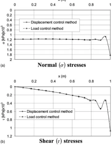
The contact normal and shear stress distributions along the soil-footing interface as obtained by the two methods at failure are presented in Figs. 5共a and b兲. They show nearly identical results. Except at the footing edge which is a singular point, a quasi-uniform normal stress distribution was observed关Fig. 5共a兲兴. For the shear stress distribution, gradually increasing stress from the center to the edge of the footing was noticed关Fig. 5共b兲兴. As for the normal stress distribution, high stresses were observed at the footing edge due to the singularity at this point.

For computation of the ultimate bearing capacity of a rough rigid footing, the displacement control method was found to be the most simple and efficient one regarding the computation time. It will be used in this paper for all subsequent calculations.

Serviceability Limit State—Vertical Displacement

For the computation of the vertical displacement of a rigid footing under an applied vertical load, it would not be interesting to apply uniform stresses directly to the surface nodes of the soil since this approach corresponds to the simulation of a flexible footing. Thus, as in the ultimate limit state, modeling the foundation by a weightless elastic material is also adopted here. An elastic-perfectly plastic model is used for the soil since it enables the development of plastic zones that may occur near the footing edges even at small service loads and it leads to more accurate solutions than a purely elastic model. The same procedure de-scribed before concerning the geostatic stresses is used here. A

Fig. 3.Load-displacement curve from displacement control method

Fig. 4.Load-displacement curve from load control method

Fig. 5.共a兲 Normal 共␴兲; 共b兲 shear 共␶兲 stresses at right half of footing

uniform service stress is applied at the base of the footing. Damp-ing of the system is introduced by runnDamp-ing several cycles until a steady state of static equilibrium is reached in the soil. This state is achieved when both conditions:共1兲 a constant vertical displace-ment of the footing共Fig. 6兲 and 共2兲 small values of unbalanced forces, were satisfied as the number of cycles increases.

Reliability Analysis of Strip Footings

The aim of this paper is to perform a reliability analysis of a strip footing resting on a c −␸ soil and subjected to a central vertical load. Two failure or unsatisfactory performance modes are con-sidered in the analysis: The first one involves the ultimate limit state and emphasizes the ultimate bearing capacity of the footing and the second one considers the serviceability limit state and focuses on the maximal footing displacement. The two determin-istic models presented in the previous section are used. The response surface methodology is employed to find an approxima-tion of the analytically unknown performance funcapproxima-tions. The co-hesion c, the angle of internal friction␸, the Young’s modulus E, and the Poisson’s ratio ␯ of the soil are considered as random variables. Due to the relatively low effect of the elastic modulus E and the Poisson’s ratio␯ on the ultimate bearing capacity, only c and␸ will be considered as random variables while studying the ultimate limit state. Similarly, only the randomness of E and ␯ will be taken into consideration in the analysis of the serviceabil-ity limit state. After a brief description of the performance func-tions used in the present analysis, the response surface methodol-ogy and its numerical implementation are presented. Then, the probabilistic numerical results based on this method are presented and discussed.

Performance Functions

Two performance functions are used in this reliability analysis. The first one is defined with respect to the ultimate bearing ca-pacity of the soil. It is given as follows

G = Pu/PS− 1 共4兲

where Pu⫽ultimate foundation load calculated by FLAC3D and PS⫽applied footing load. The second performance function,

de-fined with respect to a prescribed admissible footing displace-ment, is given as follows

G = umax− u 共5兲

where u⫽vertical displacement of the footing calculated by FLAC3Ddue to a service load PS; and umax⫽maximal admissible

vertical displacement.

Response Surface Method

If the performance function is an explicit function of the random variables, the reliability index can be calculated easily. In the FLAC3D _{model, the closed form solution of the performance}

function is not available. Thus, the determination of the reliability index is not straightforward. An algorithm based on the response surface methodology proposed by Tandjiria et al. 共2000兲 is used in this paper with the aim to calculate the reliability index and the corresponding design point. The basic idea of this method is to approximate the performance function by an explicit function of the random variables, and to improve the approximation via itera-tions. The approximate performance function used in this study has a quadratic form. It uses a second-order polynomial with squared terms but no cross terms. The expression of this approxi-mation is given by G共x兲 = a0+

兺

兺

where xi⫽random variables; n⫽number of the random variables;

and共ai, bi兲⫽coefficients to be determined. In this paper, two

ran-dom variables are considered for each limit state共i.e., n=2兲. They are characterized by their mean values ␮i and their coefficients

of variation ␴i. A brief explanation of the algorithm used is as

follows:

1. Evaluate the performance function G共x兲 at the mean value point ␮ and the 2n points each at ␮±k␴ where k=1in this paper;

2. The above 2n + 1 values of G共x兲 can be used to solve Eq. 共6兲 for the coefficients共ai, bi兲. This obtains a tentative response

surface function;

3. Solve Eq.共1兲 to obtain a tentative design point and a tenta-tive␤HLsubject to the constraint that the tentative response

surface function of step 2 be equal to zero; and

4. Repeat steps 1–3 until convergence. Each time step 1 is re-peated, the 2n + 1 sampled points are centered at the new tentative design point of step 3.

Numerical Implementation of Response Surface Method

As described in the previous section, the determination of the Hasofer–Lind reliability index requires: 共1兲 the determination of the coefficients 共a_i, b_i兲 of the tentative response surface via the resolution of Eq. 共6兲 for the 2n+1 sampled points; and 共2兲 the minimization of the Hasofer–Lind reliability index subject to the constraint that the tentative response surface function be equal to zero. These two operations which constitute a single iteration

Fig. 6.Vertical footing displacement versus number of cycles due to

were done using the optimization toolbox available in Matlab 7.0 software. Several iterations were performed until convergence of the Hasofer–Lind reliability index.

Notice that the determination of the performance function at the 2n + 1 sampled points was performed using deterministic FLAC3D_{calculations. The results of these computations constitute}

input parameters for the determination of the coefficients共ai, bi兲

of the tentative response surface using Matlab 7.0. Also, the value of the design point determined using the minimization procedure in Matlab 7.0 is an input parameter for the determination of the performance function at the 2n + 1 sampled points in FLAC3D_.

Therefore, an exchange of data between FLAC3D_{and Matlab 7.0}

in both directions was necessary to enable an automatic resolution of the iterative algorithm for the determination of the Hasofer– Lind reliability index. The link between FLAC3D_{and Matlab 7.0}

was performed using text files and FISH commands.

Numerical Results

For the ultimate limit state, different values of the coefficients of variation of the angle of internal friction and cohesion are pre-sented in the literature. For most soils, the mean value of the effective angle of internal friction is typically between 20 and 40°. Within this range, the corresponding coefficient of variation as proposed by Phoon and Kulhawy共1999兲 is essentially between 5 and 15%. For the effective cohesion, the coefficient of variation

共COV兲 varies between 10 and 70% 共Cherubini 2000兲. For the

coefficient of correlation, Harr 共1987兲 has shown that a correla-tion exists between the effective cohesion c and the effective angle of internal friction ␸. The results of Wolff 共1985兲 共␳c,␸ = −0.47兲, Yuceman et al. 共1973兲 共−0.49ⱕ␳c,␸ⱕ−0.24兲, Lumb

共1970兲 共−0.7ⱕ␳c,␸ⱕ−0.37兲, and Cherubini 共2000兲 共␳c,␸= −0.61兲

are among the ones cited in the literature. In this paper, the illus-trative values used for the statistical moments of the shear strength parameters and their coefficient of correlation ␳c,␸ are

given as follows: ␮c= 20 kPa, ␮␸= 30°, COVc= 20%, COV␸

= 10%, and␳c,␸= −0.5. These values are within the range of

val-ues cited above. For the probability distribution of the random variables, c is assumed to be lognormally distributed while ␸ is assumed to be bounded and a beta distribution is used 共Fenton and Griffiths 2003兲. The parameters of the beta distribution are determined from the mean value and standard deviation of␸. It should be mentioned that the soil elastic properties共i.e., K and G or E and ␯兲 considered as deterministic in the present ultimate limit state have no effect on the value of the ultimate bearing capacity. Higher values of these properties, G = 100 MPa and K = 133 MPa 共for which E=240 MPa and ␯=0.2兲, were checked. No change was observed in the value of the ultimate bearing capacity. Furthermore, a reduction by 50% in the number of cycles necessary to reach failure was noticed共i.e., a reduction in the computation time by half兲. Consequently, these values will be used in all subsequent calculations when studying the ultimate limit state. The CPU time required for each simulation was found to be about 15 min on a Centrino 2.0 GHz PC.

For the serviceability limit state, soils with small values of Young’s modulus are used in this paper. In such soils, the vari-ability of the compressibility characteristics is very large 共Bauer and Pula 2000兲. A lognormal distribution is used for E with a mean value of 60 MPa共Nour et al. 2002兲. For the coefficient of variation, some values proposed and used by several authors are listed in Table 1. A value of 15% is used in this paper. Regarding the Poisson’s ratio, there is no available information about its

random variation. Some authors have suggested that the random-ness can be neglected in an analysis of settlement taking place in the case of elastic soil. Others have stated that␯ changes with a relatively narrow interval. In this paper,␯ is considered as a log-normally distributed variable with a coefficient of variation of 5%. Its mean value is taken equal to 0.3. For the correlation coefficient of these two parameters, there is no information avail-able. The results reported by some researchers 共Bauer and Pula 2000兲 lead to the conclusion that this correlation is negative. In this paper, the cases of uncorrelated and correlated soil elastic properties with␳E,␷= −0.5 are considered. The CPU time required

for each serviceability limit state simulation was found to be about 10 min on a Centrino 2.0 GHz PC.

Ultimate Limit State

Graphical Representation of Successive Tentative Response Surfaces

Fig. 7 shows the evolution of the tentative response surface in the standard space 共u1, u2兲 for a footing applied load equal to

775 kN/m 共i.e., a safety factor of 3.1兲. The two equations used for the transformation of each 共c,␸兲 of the limit state surface from the physical space to the standardized normal uncorrelated space共u1, u2兲 are 共e.g., Lemaire 2005兲

Table 1.Values of Coefficient of Variation共COV兲 of Young’s Modulus Proposed by Several Authors

Authors

COV of Young’s modulus

共%兲

Phoon and Kulhawy共1999兲 30 Bauer and Pula共2000兲 15 Nour et al.共2002兲 40–50 Baecher and Christian共2003兲 2–42

u1=

冉

冊

冑

冋

冉

冊

冉

冊

册

where␳⫽coefficient of correlation of c and ␸; and ␮_cN,␮_␸N,␴_cN, and␴_␸N⫽equivalent normal means and standard deviations of the random variables c and␸. They are determined from the transla-tion approach using the following equatransla-tions

c −␮_cN ␴c N =⌽ −1_关F c共c兲兴 共9兲 ␸ − ␮_␸N ␴_␸N =⌽ −1_关F ␸共␸兲兴 共10兲 where Fcand F␸⫽non-Gaussian cumulative distribution functions of c and ␸; and ⌽−1_{共·兲⫽inverse of the standard normal}

cumula-tive distribution.

A convergence criterion on the reliability index was adopted. It considers that convergence is reached when a difference smaller than 10−2_{between two successive reliability indexes is achieved.}

One can notice that this criterion is reached after only four itera-tions. Thus, only 20 numerical simulations by FLAC3D_were

nec-essary. The corresponding CPU time required is about 20⫻15 = 300 min共i.e., 5 h兲. A value of 4.35 was found for the reliability index. This value corresponds to a failure probability of 6.84

⫻10−6_{calculated by the FORM approximation.}

Reliability Index and Design Point

Table 2 presents the Hasofer–Lind reliability index and the cor-responding design point for different values of the vertical applied load PS共i.e., safety factor F= Pu/ PS兲 varying from small values

up to the deterministic ultimate load. The cases of correlated

共␳c,␸= −0.5兲 and uncorrelated 共␳c,␸= 0兲 shear strength parameters

are considered.

The reliability index decreases with the increase of the applied load PS共i.e., the decrease of the safety factor F= Pu/ PS兲 until it

vanishes for an applied load equal to the deterministic ultimate load. This case corresponds to a deterministic state of failure for which F = 1 using the mean values of the random variables and the failure probability is equal to 50%. The comparison of the results of correlated variables with those of uncorrelated variables shows that the reliability index corresponding to uncorrelated variables is smaller than the one of negatively correlated vari-ables. One can conclude that the hypothesis of uncorrelated shear strength parameters is conservative in comparison to the one of negatively correlated parameters. For instance, when the safety

factor is equal to 3.2共i.e., PS= 750 kN/m兲, the reliability index

increases by 32% if the variables c and␸ are considered as nega-tively correlated.

The values of the design points corresponding to different val-ues of the vertical applied load can give an idea about the partial safety factors of each of the strength parameters c and tan␸ as follows Fc= ␮c c* 共11兲 F_␸=tan共␮␸兲 tan␸* 共12兲 Table 2 shows that for uncorrelated shear strength parameters, the values of c* and ␸* at the design point are smaller than their respective mean values and increase with the increase of the ap-plied load. Consequently, the partial safety factors Fcand F␸

de-crease with the inde-crease of the applied load. They tend to 1 when

PS= Pu. For negatively correlated shear strength parameters, c*

slightly exceeds the mean for some values of the applied load. This can be explained by the counterclockwise rotation of the dispersion ellipse due to the negative correlation 共Fig. 8兲. The position of the design point, which is the point of tangency be-tween the ellipse and the limit state surface, changes from that found for uncorrelated soil shear strength parameters. A higher c*

共respectively, a lower ␸*_{兲 is found. Consequently, c}*_{can become}

greater than the mean value for a negative correlation. This

con-Table 2.Reliability Index and Design Point for Uncorrelated and Correlated Shear Strength Parameters

␳c,␸= 0.0 ␳c,␸= −0.5 P_S 共kN/m兲 F c* 共kPa兲 ␸ * 共°兲 ␤HL Fc F␸ c* 共kPa兲 ␸ * 共°兲 ␤HL Fc F␸ 750 3.19 14.12 20.86 3.49 1.42 1.52 17.08 19.34 4.62 1.17 1.64 1,150 2.08 16.30 24.27 2.12 1.23 1.28 18.26 23.08 2.71 1.10 1.35 1,550 1.54 17.90 26.61 1.21 1.12 1.15 18.64 26.43 1.53 1.07 1.16 1,780 1.35 18.52 27.71 0.81 1.08 1.10 20.04 27.22 1.00 0.99 1.12 1,950 1.23 18.89 28.45 0.55 1.06 1.07 19.92 28.14 0.67 1.00 1.08 2,395 1.00 19.61 30.00 0.00 1.01 1.00 19.61 30.00 0.00 1.01 1.00

Fig. 8.General layout of dispersion ellipse for different correlation

clusion is similar to that found by Youssef Abdel Massih et al.

共2008兲.

Sensitivity of Failure Probability to Variability of Soil Shear Strength Parameters

In order to study the effect of the variability of the soil shear strength parameters on the failure probability, Fig. 9 shows the

FORM failure probability versus the coefficient of variation of c

and␸. For each curve, the coefficient of variation of a parameter is held to the same constant value given in the introduction of the section “Numerical Results” and the coefficient of variation of the second parameter is varied over the range 10–40%. The results show that the failure probability is highly influenced by the coef-ficient of variation of the angle of internal friction; the greater the scatter in␸ the higher the failure probability of the foundation. This means that the accurate determination of the distribution of this parameter is very important in obtaining reliable probabilistic results. In contrast, the coefficient of variation of c does not sig-nificantly affect the failure probability.

Serviceability Limit State

Reliability Index and Design Point

The threshold value of the settlement is umax= 0.1 m. Table 3

pre-sents the Hasofer–Lind reliability index and the corresponding design point for different values of the vertical applied load PS.

The cases of correlated and uncorrelated soil elastic properties are considered. The reliability index decreases with the increase of the applied load PS. A comparison of the results of correlated soil

elastic properties with those of uncorrelated ones shows that, as in

the ultimate limit state, the hypothesis of uncorrelated soil elastic properties is conservative in comparison to the one of negatively correlated properties.

By comparing Tables 2 and 3, one can notice that for small values of the applied load, the reliability index of the ultimate limit state is significantly smaller than that of the serviceability limit state. Thus, for small values of the applied load, the ultimate failure mode is predominant and will have the highest contribu-tion in the determinacontribu-tion of the system failure probability. The difference between the reliability indexes of the two failure modes becomes smaller for higher values of the applied load. Consequently, when the applied load increases, the two failure modes 共i.e., the ultimate and the serviceability ones兲 will have nearly similar contributions in the computation of the system fail-ure probability共see another interpretation in the section “System Failure Probability”兲.

As for the ultimate limit state, the values of the design point allow us to calculate the partial safety factors of E and ␯ as follows FE= ␮E E* 共13兲 F_␷=␮␯ ␯* 共14兲

Table 3 shows that for uncorrelated soil elastic properties, the partial safety factors FEand F␯decrease with the increase of PS.

They become equal to 1 when PSis equal to the load that leads to

the maximal prescribed foundation settlement umaxfor the mean

values of the soil elastic properties. For negatively correlated soil elastic properties, F_␯is found smaller than 1. The same interpre-tation given in the ultimate limit state for negatively correlated variables remains valid in the present case.

Sensitivity of Failure Probability to Variability of Soil Elastic Properties

As for the ultimate limit state, the effect of the variability of the soil elastic properties on the failure probability is shown in Fig. 10 where FORM failure probability is plotted versus the coeffi-cient of variation of E and ␯. For each curve, the coefficient of variation of a parameter is held to the same constant value given in the introduction of the section “Numerical Results” and the coefficient of variation of the second parameter is varied over the range 5–35%. The results show that the failure probability of the serviceability limit state is highly influenced by the coefficient of variation of the Young’s modulus; the greater the scatter in E the higher the failure probability of the foundation. This means that an accurate determination of the distribution of this parameter is very important in obtaining reliable probabilistic results. In

con-Fig. 9.Effect of variability of soil shear strength parameters on

fail-ure probability

Table 3.Reliability Index and Design Point for Uncorrelated and Correlated Soil Elastic Properties

␳E,␷= 0.0 ␳E,␷= −0.5 PS 共kN/m兲 E* 共MPa兲 ␷* _␤ HL FE F␷ E* 共MPa兲 ␷* _␤ HL FE F␷ 750 19.42 0.280 7.60 3.10 1.07 16.57 0.337 8.80 3.62 0.89 1,150 33.71 0.288 3.87 1.78 1.04 31.06 0.319 4.46 1.93 0.94 1,550 49.75 0.296 1.21 1.21 1.01 48.37 0.306 1.41 1.24 0.98 1,780 59.33 0.300 0.00 1.01 1.00 59.33 0.300 0.00 1.01 1.00

trast, compared to E, the uncertainties in␯ have a minor effect on the failure probability.

System Failure Probability

The system failure probability under the two failure modes in-volving the ultimate and the serviceability limit states of the foot-ing is given by

Pf_sys= Pf共U 艛 S兲 = Pf共U兲 + Pf共S兲 − Pf共U 艚 S兲 共15兲

where Pf共U艚S兲⫽failure probability under the ultimate and the

serviceability failure modes; Pf共U兲⫽failure probability under

only the ultimate failure mode; and Pf共S兲⫽failure probability

under only the serviceability failure mode. The failure probability of the intersection is given as follows共Lemaire 2005兲

max共P共A兲,P共B兲兲 ⱕ Pf共P 艚 S兲 ⱕ P共A兲 + P共B兲 共16兲

where P共A兲 = ⌽共− ␤U兲⌽

冉

冑

冊

冉

冑

冊

␤Uand␤S⫽reliability indexes corresponding to the ultimate and

the serviceability failure modes, respectively, and ␳US

⫽cor-relation between the two failure modes.␣_Uand␣_Sfor both modes are given by ␣U_i= −

冏

冏

冏

冏

*_{⫽standard uncorrelated normal variables at the}

design points关see Eqs. 共7兲 and 共8兲兴. Here, it was found that ␳US

= 0 since the two failure modes are independent.

The probability of the intersection Pf共U艚S兲 is set equal to its

lower limit关i.e., max共P共A兲, P共B兲兲兴 in order to obtain the higher limit of the system failure probability Pf_sys.

The system reliability index can be approximated using the

FORM approximation as follows

␤sys= −⌽−1共Pfsys兲 共22兲

Table 4 presents the system failure probability Pfsysand the

cor-responding reliability index␤sysfor different values of the applied

load. Four cases are considered: They are the combinations of correlated and uncorrelated shear strength parameters with corre-lated and uncorrecorre-lated soil elastic properties. From this table, it can be seen that even for the system reliability, the assumption of uncorrelated parameters is conservative in comparison to the one of negatively correlated variables. For small values of the applied load, where the ultimate failure mode is predominant, one can notice that the system reliability index is equal to the reliability index of the ultimate failure mode. When the applied load in-creases, the system reliability depends on both failure modes and the system reliability index is smaller than the ones corresponding to a single failure mode. Finally, one can notice that a negative system reliability index is found for an applied load of 1,780 kN/m corresponding to the deterministic failure state of the serviceability mode. This corresponds to a system failure prob-ability higher than 50%共i.e., higher than the one corresponding to a zero reliability index兲. This value is due to the combination of the failure probability of the serviceability limit state共i.e., 50%兲 and the one of the ultimate limit sate. In this case, the system reliability index is meaningless.

Conclusions

A reliability-based analysis of a strip footing resting on a c −␸ soil and subjected to a central vertical load is presented. Both the ultimate and the serviceability limit states are used to characterize the footing behavior. Two deterministic models based on

numeri-Fig. 10. Effect of variability of soil elastic properties on failure

probability

Table 4.System Failure Probability and Reliability Index

␳c,␸= 0.0 ␳E,␷= 0.0 ␳c,␸= −0.5 ␳E,␷= −0.5 ␳c,␸= −0.5 ␳E,␷= 0.0 ␳c,␸= 0.0 ␳E,␷= −0.5 PS 共kN/m兲 Pfsys 共%兲 ␤sys Pf_sys 共%兲 ␤sys Pf_sys 共%兲 ␤sys Pf_sys 共%兲 ␤sys 750 0.02 3.49 2.00⫻10−4 4.62 2.00⫻10−4 4.62 0.02 3.49 1,150 1.70 2.12 0.34 2.71 0.34 2.70 1.70 2.12 1,550 21.30 0.79 13.70 1.09 16.90 0.96 18.30 0.90 1,780 60.45 −0.26 57.93 −0.20 57.93 −0.20 60.45 −0.26

cal simulations using the Lagrangian explicit finite difference code FLAC3D_{are employed. The first one computes the ultimate}

bearing capacity of the foundation and the second one calculates the footing displacement due to an applied service load. The Hasofer–Lind reliability index is adopted here for the assessment of the foundation reliability. The response surface methodology is used to find an approximation of the analytically unknown limit state surfaces and the corresponding reliability indexes. Only the soil shear strength parameters are considered as random variables while studying the ultimate limit state. Also, the randomness of only the soil elastic properties is taken into account in the service-ability limit state. The main conclusions of this paper can be summarized as follows:

1. The hypothesis of uncorrelated parameters was found to be conservative in comparison to the one of negatively corre-lated variables;

2. For uncorrelated shear strength parameters, the values of c* and␸* at the design point are found smaller than their re-spective mean values and increase with the increase of the applied load PS. Consequently, the partial safety factors Fc

and F_␸decrease with the increase of the applied load. They tend to 1 when PS= Pu. For negatively correlated shear

strength parameters, c* slightly exceeds the mean for some values of the applied load;

3. For uncorrelated soil elastic properties, the partial safety fac-tors F_Eand F_␯decrease with the increase of P_S. They tend to 1 when PS is equal to the load that leads to the maximal

prescribed foundation settlement umaxfor the mean values of

the soil elastic properties. For negatively correlated soil elas-tic properties, F_␯is found smaller than 1;

4. The failure probability is found to be highly influenced by the uncertainties of the angle of internal friction for the ulti-mate limit state and by those of the Young’s modulus for the serviceability limit state; and

5. For small values of the applied load, the ultimate limit state is predominant in the computation of the system failure prob-ability. Consequently, the system reliability index is found equal to that of the ultimate limit state. For higher values of the applied load, the system reliability index depends on both limit states. It is smaller than the ones corresponding to a single failure mode. Thus, both failure modes have to be considered in the reliability analysis of foundations for high values of the applied load.

Acknowledgments

The writers would like to thank the Lebanese National Council for Scientific Research 共CNRSL兲 and the French organization EGIDE for providing the financial support for this research.

References

Baecher, G., and Christian, J.共2003兲. Reliability and statistics in

geotech-nical engineering, Wiley, U.K.

Bauer, J., and Pula, W. 共2000兲. “Reliability with respect to settlement limit-states of shallow foundations on linearly-deformable subsoil.”

Comput. Geotech., 26, 281–308.

Cherubini, C.共2000兲. “Reliability evaluation of shallow foundation bear-ing capacity on c⬘,␸⬘soils.” Can. Geotech. J., 37, 264–269.

Ditlevsen, O.共1981兲. Uncertainty modelling: With applications to

multi-dimensional civil engineering systems, McGraw-Hill, New York.

Fenton, G. A., and Griffiths, D. V. 共2002兲. “Probabilistic foundation settlement on spatially random soil.” J. Geotech. Geoenviron. Eng.,

128共5兲, 381–390.

Fenton, G. A., and Griffiths, D. V.共2003兲. “Bearing capacity prediction of spatially random C-␸ soils.” Can. Geotech. J., 40, 54–65.

Fenton, G. A., and Griffiths, D. V.共2005兲. “Three-dimensional probabi-listic foundation settlement.” J. Geotech. Geoenviron. Eng., 131共2兲, 232–239.

FLAC3D_{.共1993兲. Fast Lagrangian analysis of continua, ITASCA} Con-sulting Group, Inc., Minneapolis.

Griffiths, D. V., and Fenton, G. A.共2001兲. “Bearing capacity of spatially random soil: the undrained clay Prandtl problem revisited.”

Geotech-nique, 51共4兲, 351–359.

Griffiths, D. V., Fenton, G. A., and Manoharan, N. 共2002兲. “Bearing capacity of rough rigid strip footing on cohesive soil: Probabilistic study.” J. Geotech. Geoenviron. Eng., 128共9兲, 743–755.

Harr, M. E. 共1987兲. Reliability-based design in civil engineering, McGraw-Hill, New York.

Hasofer, A. M., and Lind, N. C. 共1974兲. “Exact and invariant second-moment code format.” J. Engrg. Mech. Div., 100共1兲, 111–121. Lemaire, M.共2005兲. Fiabilité des structures, Hermès, Lavoisier, Paris 共in

French兲.

Low, B. K.共2005兲. “Reliability-based design applied to retaining walls.”

Geotechnique, 55共1兲, 63–75.

Low, B. K., and Phoon, K. K. 共2002兲. “Practical first-order reliability computations using spreadsheet.” Proc., Probabilistics in

Geotech-nics: Technical and Economic Risk Estimation, Verlag Gluckauf

GmbH. Essen, Graz, Austria, 39–46.

Low, B. K., and Tang, W. H. 共1997a兲. “Efficient reliability evaluation using spreadsheet.” J. Eng. Mech., 123共7兲, 749–752.

Low, B. K., and Tang, W. H.共1997b兲. “Reliability analysis of reinforced embankments on soft ground.” Can. Geotech. J., 34, 672–685. Low, B. K., and Tang, W. H.共2004兲. “Reliability analysis using

object-oriented constrained optimization.” Struct. Safety, 26, 68–89. Lumb, P.共1970兲. “Safety factors and the probability distribution of soil

strength.” Can. Geotech. J., 7, 225–242.

Nour, A., Slimani, A., and Laouami, N.共2002兲. “Foundation settlement statistics via finite element analysis.” Comput. Geotech., 29, 641– 672.

Phoon, K.-K., and Kulhawy, F. H.共1999兲. “Evaluation of geotechnical property variability.” Can. Geotech. J., 36, 625–639.

Popescu, R., Deodatis, G., and Nobahar, A. 共2005兲. “Effect of random heterogeneity of soil properties on bearing capacity.” Probab. Eng.

Mech., 20, 324–341.

Przewlocki, J.共2005兲. “A stochastic approach to the problem of bearing capacity by the method of characteristics.” Comput. Geotech., 32, 370–376.

Tandjiria, V., Teh, C. I., and Low, B. K.共2000兲. “Reliability analysis of laterally loaded piles using response surface methods.” Struct. Safety,

22, 335–355.

Wolff, T. H.共1985兲. “Analysis and design of embankment dam slopes: A probabilistic approach.” Ph.D. thesis, Purdue Univ., Lafayette, Ind. Yin, J.-H., Wang, Y.-J., and Selvadurai, P. S.共2001兲. “Influence of

non-associativity on the bearing capacity of a strip footing.” J. Geotech.

Geoenviron. Eng., 127共11兲, 985–989.

Youssef Abdel Massih, D. S., Soubra, A.-H., and Low, B. K. 共2008兲. “Reliability-based analysis and design of strip footings against bear-ing capacity failure.” J. Geotech. Geoenviron. Eng., in press. Yuceman, M. S., Tang, W. H., and Ang, A. H. S.共1973兲. “A probabilistic

study of safety and design of earth slopes.” Civil engineering studies, Structural Research Series 402, University of Illinois Press, Urbana, Ill.