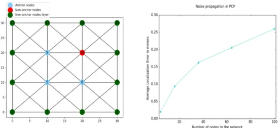
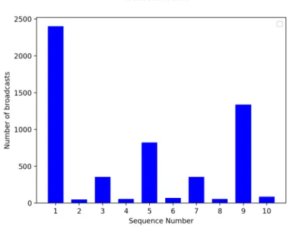
Position certainty propagation: a localization service for Ad-Hoc Networks
Texte intégral
Figure

Documents relatifs
The influence on the energy consumption of a sensor node of the following param- eters of ubiquitious sensor network: the density of distribution of smart things in the network
We study the probability of selling a product containing social or environmental claims based on different levels of cues (the non-verifiable green communication) and hard
In contrast to the solutions presented in [8], [9], [10], which deal with stabilizing the aerial vehicle in hover or in take- off and landing tasks, the research presented in this
Cependant, dans la majorité des travaux de prothèse esthétique, le choix de la teinte des céramiques et des résines composites est basé sur une compréhension profonde de
[ 45 ] 41 10–20 Chiari osteotomy 4.0 (7.2) Improved Harris hip score, improvement of acetabular angle of Sharp, increase of LCE angle, improved femoral head coverage,
Quality of service forest (QoS-F) is a distributed algorithm to construct a forest of high quality links (or nodes) from net- work point of view, and use these for routing
In this innovative biomechanical study, we compare the impact of two kinds of squatting position flexion accord- ing to the position of the feet (flat versus on tiptoe) on
in such scenario, the position of the destination node may be easily assumed to be known. The use of positioning information in DYMO- selfwd is expected to reduce the routing
