Généralisation des précodeurs MIMO basés sur la distance euclidienne minimale

HAL Id: tel-00839594

https://tel.archives-ouvertes.fr/tel-00839594v2

Submitted on 28 Jun 2013

HAL is a multi-disciplinary open access

archive for the deposit and dissemination of sci-entific research documents, whether they are pub-lished or not. The documents may come from teaching and research institutions in France or abroad, or from public or private research centers.

L’archive ouverte pluridisciplinaire HAL, est destinée au dépôt et à la diffusion de documents scientifiques de niveau recherche, publiés ou non, émanant des établissements d’enseignement et de recherche français ou étrangers, des laboratoires publics ou privés.

distance euclidienne minimale

Quoc-Tuong Ngo

To cite this version:

Quoc-Tuong Ngo. Généralisation des précodeurs MIMO basés sur la distance euclidienne minimale. Traitement du signal et de l’image [eess.SP]. Université Rennes 1, 2012. Français. �tel-00839594v2�

THÈSE / UNIVERSITÉ DE RENNES 1

sous le sceau de l’Université Européenne de Bretagne

pour le grade de

DOCTEUR DE L’UNIVERSITÉ DE RENNES 1

Mention : Traitement du Signal et Télécommunications

École doctorale MATISSE

présentée par

Quoc-Tuong NGO

préparée à l’unité de recherche UMR6074 IRISA

Institut de recherche en informatique et systèmes aléatoires - CAIRN

École Nationale Supérieure des Sciences Appliquées et de Technologie

Generalized minimum

Euclidean distance

based precoders for

MIMO spatial

multiplexing systems

Thèse soutenue à Lannion le 17 janvier 2012

devant le jury composé de :

CANCES Jean-Pierre

Professeur à l’Université de Limoges / rapporteur

SLOCK Dirk

Professeur à EURECOM / rapporteur

BUREL Gilles

Professeur à l’Université de Bretagne Occidentale / examinateur

DIOURIS Jean-FranŊois

Professeur à l’Université de Nantes / examinateur

SCALART Pascal

Professeur à l’Université de Rennes 1 / directeur de thèse

BERDER Olivier

Maître de Conférences à l’Université de Rennes 1/ co-directeur de thèse

like any great relationship, it just gets better and better as the years roll on."

The three year graduate work in IRISA/CAIRN Lab is a most memorial period in my life, not only because I have been led to an exciting field, the MIMO precoding techniques which were totally new to me before, but also I have got the opportunity to study and work in a very dynamic laboratory .

Firstly, I would like to thank my supervisor Prof. Pascal Scalart and co-supervisor Olivier Berder for their consistent supervision and encouragement throughout my study and research, their patient guidance on direction of my work. All of their feedbacks, suggestions, and gentleness at various stages have been significantly improved my knowl-edges, scientific minds, and skills of writing and presentation.

I would also like to thank all the members of the jury for reading part of my thesis: Prof. Jean-Pierre CANCES at the University of Limoges, Prof. Dirk SLOCK at the EURECOM (Nice) , Prof. Gilles BUREL at the University of Bretagne Occidentale, and Prof. Jean-Françoisand DIOURIS at the University of Nantes. Their suggestions and comments are really appreciated.

I am most grateful to Prof. Oliver Sentieys, the head of CAIRN Lab, for his kind attitude and constant willingness to help makes my graduate study a very enjoyable experience. I also want to thank all of my friends in Lannion who make my stay a memorial period. My warmest thanks also go to my parents for their never ending support. They always assist me in implementing my desires.

Finally, I would like to say something special to my girlfriends. She is a powerful emo-tional support that I can share my burdens, fears and sadness. Thanks you for her understanding, her helps, and her endless love.

Contents

Acknowledgements i

Abbreviations vi

List of Figures viii

List of Tables xi

Introduction 1

1 Wireless communication and MIMO technology 5

1.1 Transmission channel . . . 6 1.1.1 Path loss . . . 6 1.1.2 Fading . . . 7 1.2 Diversity technique. . . 9 1.2.1 Temporal diversity . . . 9 1.2.2 Frequency diversity . . . 9 1.2.3 Spatial diversity . . . 10 1.2.4 Antenna diversity . . . 10

1.3 Multiple-Input Multiple-Output techniques . . . 11

1.3.1 Basic system model . . . 12

1.3.2 MIMO channel capacity . . . 13

1.4 Space Time Coding . . . 14

1.4.1 Alamouti Code. . . 15

1.4.2 Orthogonal Space-Time Block Codes. . . 16

1.4.3 Quasi-Orthogonal Space-Time Block Codes. . . 17

1.4.4 Space Time Trellis Codes . . . 18

1.5 Precoding technique . . . 19

1.5.1 Encoding structure . . . 19

1.5.2 Linear precoding structure . . . 20

1.5.3 Receiver structure . . . 21

1.6 Conclusion . . . 24

2 MIMO linear precoding techniques 25 2.1 Virtual transformation. . . 26

2.1.1 Noise whitening . . . 27

2.1.2 Channel diagonalization . . . 28

2.1.3 Dimensionality reduction. . . 29 ii

2.1.4 Virtual channel representaion . . . 29

2.2 Existing precoders . . . 31

2.2.1 Beamforming or max-SNR precoder . . . 31

2.2.2 Water-Filling precoder . . . 32

2.2.3 Minimum Mean Square Error precoder . . . 32

2.2.4 Quality of Service precoder . . . 34

2.2.5 Equal Error precoder . . . 34

2.2.6 Minimum BER diagonal precoder . . . 35

2.2.7 X- and Y-codes precoder . . . 36

2.2.8 Tomlinson-Harashima precoder . . . 37

2.3 Minimum Euclidean distance based precoder . . . 39

2.3.1 Minimum Euclidean distance . . . 39

2.3.2 Parameterized form for 2-D virtual subchannels . . . 40

2.3.3 Optimal solution for QPSK modulation . . . 40

2.4 Comparison of linear precoders . . . 42

2.4.1 Comparison of minimum Euclidean distance . . . 42

2.4.2 Bit-Error-Rate performance . . . 45

2.5 Conclusion . . . 46

3 Extension of max-dmin precoder for high-order QAM modulations 48 3.1 Optimized max-dmin precoder for 16-QAM modulation . . . 49

3.1.1 Expression of the max-dmin precoder . . . 50

3.1.2 Received constellation of the max-dmin precoder . . . 55

3.1.3 Evolution of the minimum Euclidean distance . . . 55

3.1.4 Performance of the max-dmin precoder for 16-QAM modulation. . 58

3.2 General expression of max-dmin precoder for high-order QAM modulations 60 3.2.1 Precoder F1 . . . 61

3.2.2 Precoder F2 . . . 62

3.2.3 Channel threshold γ0 . . . 65

3.3 Performance for high-order QAM modulations . . . 66

3.3.1 Comparison of minimum Euclidean distance . . . 66

3.3.2 Diversity order of max-dmin precoder. . . 68

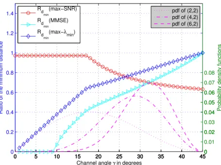
3.3.3 Distribution of the channel angle and max-dmin precoder. . . 70

3.3.4 Bit-Error-Rate performance . . . 71

3.4 Conclusion . . . 73

A Proof of Proposition 3.1 . . . 74

B Proof of Proposition 3.2 . . . 74

C Maximum value of the distance dmin . . . 77

4 Extension of max-dmin precoder for large MIMO systems 79 4.1 Cross-form precoding matrix for large MIMO systems . . . 80

4.1.1 Principle of E-dmin precoder . . . 80

4.1.2 Performance for large MIMO systems . . . 82

4.2 Three-Dimensional max-dmin precoder . . . 84

4.2.1 Parameterized form of the three-dimensional max-dmin precoder . 85 4.2.2 Optimal max-dmin precoder for a BPSK modulation . . . 87

4.2.4 Range of definition for precoders Fqc1, Fqc2 and Fqc3 . . . 93

4.2.5 Simulation results . . . 94

4.3 Extension of max-dminprecoder for large MIMO system with an odd num-ber of datastreams . . . 101

4.3.1 General form of 3-D max-dmin precoder for QAM modulations . . 101

4.3.2 Extension of 3-D max-dmin precoder for large MIMO systems . . . 103

4.3.3 BER performance for large MIMO systems . . . 104

4.4 Conclusion . . . 104

A Proof of Proposition 4.1 . . . 106

B Proof of Proposition 4.2 . . . 108

C Exact values of the Fbc2 angles. . . 110

D Proof of Proposition 4.3 . . . 111

E Expressions of the precoder Fqc2 & Fqc3 . . . 112

F Proof of Proposition 4.4 . . . 114

5 Reducing the number of neighbors for max-dmin precoder 115 5.1 Error probability of the linear precoding strategy. . . 116

5.2 Parameterization of the Neighbor-dmin precoding matrix . . . 118

5.3 Expression of Neighbor-dmin precoder for 2 sub-streams . . . 120

5.3.1 For BPSK modulation . . . 121

5.3.2 For QPSK modulation . . . 122

5.3.3 General expression for high-order QAM modulations . . . 124

5.3.4 Performance of Neighbor-dmin precoder . . . 127

5.4 Neighbor-dmin precoder for three parallel datastreams . . . 131

5.4.1 Precoder F1 . . . 132

5.4.2 Precoder F2 . . . 132

5.4.3 Precoder F3 . . . 133

5.4.4 Simulation results . . . 134

5.5 Neighbor-dmin precoder for large MIMO systems . . . 136

5.5.1 Principles . . . 136 5.5.2 Simulation results . . . 137 5.6 Conclusion . . . 138 A Proof of Lemma 5.1 . . . 140 B Proof of Lemma 5.2 . . . 141 C Proof of Proposition 5.3 . . . 142

6 Generalized precoding designs using Discrete Fourier Transform ma-trix 143 6.1 Parameterization of the precoding matrix . . . 144

6.2 Design of the precoding matrix . . . 147

6.2.1 Principle of the approach. . . 147

6.2.2 Design model . . . 150

6.3 Optimized precoder for rectangular QAM modulations . . . 151

6.3.1 Expressions of the precoder . . . 152

6.3.2 Range of definition . . . 157

6.4 Simulation results . . . 158

6.4.2 Bit-Error-Rate performance . . . 159

6.5 Conclusion . . . 163

Abbreviations

≃ approximately equal to

A∗ Hermitian (complex and conjugate) of matrix A

AT transpose of matrix A

A+ pseudo inverse of matrix A

E{x} expectation of x

Ib Identity matrix of size b × b

∥x∥ vector 2-norm

˘

x difference vector

ˆ

x detected symbol, or estimated value of x

∥F∥ Frobenius norm of matrix F

diag{x1, x2, ⋯, xn} diagonal matrix with n diagonal elements x₁, x₂, ⋯, x_n

nT number of transmit antennas

nR number of receive antennas

ns= ∣n_T −n_R∣ asymmetric coefficient

Es average transmit power for nT transmit antennas

b number of datastreams

H [n_R×n_T] channel matrix

F [nT ×b] precoding matrix

G [b × n_R] decoding matrix

s [b × 1] transmitted symbol vector

η [b × 1] additive noise vector

Hv [b × b] virtual channel matrix

Fv [nT ×b] diagonalization matrix at the transmitter

Gv [b × n_R] diagonalization matrix at the receiver

Fd [b × b] precoding matrix for virtual channel

Gd [b × b] decoding matrix for virtual channel

C channel capacity

SNR Signal to Noise ratio

dmin minimum Euclidean distance of the received constellation

¯

dmin normalized minimum Euclidean distance

γ angle of the virtual channel for two substreams

ρ gain of the virtual channel for two substreams

List of Figures

1.1 Principle of temporal diversity and frequency diversity . . . 10

1.2 MIMO model with nT transmit antennas and nR receive antennas . . . . 13

1.3 The ergodic capacity of MIMO channels.. . . 14

1.4 Alamouti encoding scheme. . . 15

1.5 Four state STTC with two transmit antennas, using 4-PSK modulation. . 18

1.6 Precoding system structure. . . 19

1.7 A multiplexing encoding structure. . . 19

1.8 A space-time encoding structure. . . 20

1.9 A linear precoding structure. . . 21

1.10 Principle of sphere decoding technique. . . 23

2.1 Virtual model of MIMO systems. . . 26

2.2 Block diagram of a MIMO system: basic model (a), diagonal transmission model (b). . . 30

2.3 Diagonal precoding schema using maximum likelihood detection (ML) at the receiver. . . 31

2.4 Algorithm of Water-Filling precoder. . . 33

2.5 Block diagram of linear precoder and matrix DFE.. . . 38

2.6 Received constellation on the first subchannel for the precoder Fr1.. . . . 42

2.7 Received constellation on the first subchannel for the precoder Focta.. . . 43

2.8 Received constellation on the second subchannel for the precoder Focta. . 43

2.9 Normalized minimum Euclidean distance for QPSK modulation. . . 44

2.10 Comparison of the minimum Euclidean distance. . . 45

2.11 Uncoded BER performance for QPSK modulation.. . . 46

3.1 The received constellation on the first virtual subchannel for ψ = 0. . . 50

3.2 Euclidean distance with ϕ = 45o _{and θ = 45}o _{for some difference vectors} with respect to ψ in degrees for channel angle γ = 30o_{.. . . . 54}

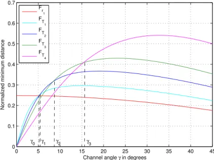
3.3 Received constellation for the precoder FT4 . . . 56

3.4 The received constellation obtained by the precoder Fr1 . . . 57

3.5 Evolution of dmin with respect to γ for a 16-QAM modulation . . . 57

3.6 Comparison in terms of the minimum Euclidean distance. . . 58

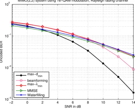
3.7 Comparison the performance in terms of BER for 16-QAM modulation. . 59

3.8 Received constellation of the precoder F1. . . 62

3.9 Received constellation of the precoder F2. . . 64

3.10 Normalized minimum Euclidean distance. . . 66

3.11 Normalized minimum Euclidean distance for 64-QAM. . . 68

3.12 Probability density functions of the angles γ. . . 71 viii

3.13 Comparison the performance in terms of BER for 64-QAM modulation. . 72

4.1 System model E-dmin solution. . . 81

4.2 BER performance for large MIMO systems. . . 83

4.3 BER performance for perfect CSI and imperfect CSI estimations. . . 84

4.4 Received constellation for the precoder Fbc1. . . 88

4.5 Received constellation for the precoder Fbc2. . . 89

4.6 Range of definition for precoders Fbc1 and Fbc2. . . 90

4.7 Received constellation for the precoder Fqc1. . . 91

4.8 Received constellation for the fourth expression of the precoder Fqc2.. . . 92

4.9 Range of definition for QPSK modulation. . . 94

4.10 Normalized Euclidean distance dmin for BPSK. . . 95

4.11 Normalized Euclidean distance dmin for QPSK modulation with γ2=45o. 96 4.12 Comparison of precoders in terms of BER for BPSK modulation with a MIMO (3,3) uncorrelated Rayleigh fading channel.. . . 97

4.13 Comparison of precoders in terms of BER for QPSK modulation with a MIMO (3,3) uncorrelated Rayleigh fading channel.. . . 98

4.14 Probability density functions of the angles γ1 and γ2 for a MIMO system with uncorrelated Rayleigh fading channel (estimation with 106 _random matrices). . . 98

4.15 BER simulation of the precoder max-dmin compared to the max-λmin and max-SNR with MIMO uncorrelated Rayleigh fading channels. . . 99

4.16 Comparison of precoders in terms of BER for perfect CSI and imperfect CSI estimation. . . 100

4.17 Comparison of precoders in terms of BER for MIMO(5,5) system. . . 105

5.1 Received constellation of the precoder Frec for QPSK. . . 124

5.2 Received constellation provided by the precoder F2. . . 126

5.3 Normalized minimum distance for the precoder Neighbor-dmin. . . 127

5.4 Normalized minimum Euclidean distance for QPSK. . . 128

5.5 BER comparison of max-dmin and Neighbor-dmin precoders. . . 129

5.6 Uncoded BER performance for QPSK modulation.. . . 129

5.7 Comparaison dmin pour MAQ-16. . . 130

5.8 Comparaison des précodeurs pour MIMO(3,2). . . 130

5.9 Received constellations provided by precoder F3 for QPSK modulation. . 134

5.10 Range of definition for the three precoders F1, F2, and F3 using a QPSK modulation. The arrows represent the evolution of the borders when the modulation order increases.. . . 135

5.11 Normalized minimum distance for QPSK. . . 136

5.12 Uncoded BER for MIMO(4,3) system using QPSK modulation. . . 137

5.13 Uncoded BER for large MIMO system using QPSK modulation. . . 138

6.1 Design model of the precoding matrix . . . 151

6.2 Received constellation for the precoder F2. . . 153

6.3 Received constellations provided by precoder F3.. . . 155

6.4 Normalized minimum Euclidean distance for two datastreams and 4-QAM modulation, with the channel angle γ = atan√ρ2/ρ1. . . 160

6.6 Comparison of BER performance for large MIMO(5,4) systems. . . 162

List of Tables

1.1 Empirical power drop-off values . . . 6

2.1 Steps to obtain the diagonal MIMO system in the case of CSIT . . . 27

3.1 Comparison of the minimum Euclidean distances. . . 67

3.2 Percentage of use F1 for uncorrelated Rayleigh fading channels. . . 71

4.1 Optimized angles in degree for the precoders Fqc2 and Fqc3 . . . 93

4.2 Percentage of use for precoder max-dminwith uncorrelated Rayleigh fadding channels. . . 99

5.1 Optimized angles for the precoder F2 . . . 133

6.1 Optimized coefficients of the power allocation matrix Σ. . . 152

6.2 Comparison of the minimum Euclidean distances. . . 159

Introduction

In the early decade of this century, it is apparent that wireless communication technolo-gies have an exponential growth. Various communication techniques have been employed to serve various demands of high-speed wireless links such as higher data rate, increased robustness, and greater user capacity. The next generation of wireless communications is based on an all-IP switched network and can provide a peak data rate up to hundreds of Mbits/s for high mobility, and to Gbits/s for low-mobility end-users. For instance, the Wi-Fi standard (IEEE 802.11n) can provide a data rate up to 600 Mbps in physical layer, and the Wi-Max standard (IEEE 802.16) can support a gross data rate up to 100 Mbps for mobile network.

One of the most well-known techniques for wireless communications is multiple-input multiple-output orthogonal frequency division multiplexing (MIMO-OFDM). This tech-nique not only offers diversity and capacity gains but also achieves higher spectral ef-ficiency and higher link reliability in comparison with single antenna or single carrier systems. The benefits of MIMO communication are generally ensured by both open-loop and closed-open-loop MIMO techniques. The open-open-loop techniques, such as space time coding (STC) and spatial multiplexing (SM), are used without the need for channel state information (CSI) at the transmitter. In order to overcome the multipath effect and improve the robustness of spatial multiplexing systems, linear precoding closed-loop techniques can be used at the transmitter. The principle of the precoding techniques is that, when the channel knowledge is available at the transmitter, the transmit signal is pre-multiplied by a precoding matrix such that the inter-symbol interference (ISI) in the receiver is greatly reduced.

The channel state information at the transmitter (CSIT) can be obtained through the feedback links, but it is difficult to achieve perfect CSIT in a MIMO system with a rapidly

changing channel. Therefore, the transmitters in many MIMO systems have no knowl-edge about the current channel. This motivates the use of limited feedback precoding methods such as channel quantization and codebook designs. The key of this method is that the optimal precoding matrix is constrained to a number of distinct matrices, which are referred to codebook entries, and known a priori to both the transmitter and receiver. Many precoding codebooks can be proposed in order to optimizing different criteria of the precoded system, and the receiver defines the optimal precoding matrix based on the current channel conditions. Since the codebook is also known at the transmitter, the receiver only needs to feedback a binary index of the optimal precoding matrix, rather than the entire precoding matrix itself. The limited feedback precoding technique is already used in Wi-Max standard (802.16e) with two codebooks: one with 8 entries and the other with 64 entries. These codebooks correspond respectively to 3-bit and 6-bit indices for each precoding matrix.

Considering the CSI from the receiver, antenna power allocation strategies can be per-formed thanks to the joint optimization of linear precoder (at the transmitter) and decoder (at the receiver) according to various criteria such as maximizing the output ca-pacity, maximizing the received signal-to-noise ratio (SNR), minimizing the mean square error (MSE), minimizing the bit error rate (BER), or maximizing the minimum singular value of the channel matrix. These optimized precoding matrices are diagonal in the vir-tual channel representation and belong to an important set of linear precoding techniques named diagonal precoders. Another group of precoding techniques is obviously the non-diagonal linear structure. One of the most efficient non-non-diagonal precoder is based on the maximization of the minimum Euclidean distance (max-dmin) between two received

data vectors. The max-dmin precoder offers a significant improvement in terms of BER

compared to other precoding strategies. Since the minimum distance based transceiver needs a Maximum-Likelihood (ML) detector, the complexity of max-dmin precoder is

fairly complicated. Furthermore, it is difficult to define the closed-form of the optimized precoding matrix for large MIMO system with high-order modulations. In this thesis, we will study the performances, and propose some extensions of the max-dmin solution.

Following this introduction, this document is organized as follows: Chapter 1

In this chapter, the propagation over wireless channels is firstly presented. The principles and different types of diversity techniques are then investigated. A brief introduction of the MIMO technologies with capacity and diversity gains are referred, and the space time coding technique is described. Finally, the precoding system structure which consists of an encoder, a precoder and a decoder is presented.

Chapter 2

A virtual transformation is used to diagonalize the channel matrix, and the principles of some existing precoders are presented in the chapter. The performance of the max-dmin

precoder in terms of minimum distance and bit-error-rate is also considered in comparison with other precoders.

Chapter 3

The max-dmin solution was only available in closed-form for two independent

data-streams with low-order modulations (BPSK and QPSK). That is due to the expression of the distance dminthat depends on the number of data-streams, the channel

character-istics, and the modulation. Therefore, we present the optimized solution of the max-dmin

precoder for two 16-QAM symbols. This new strategy selects the best precoding matrix among five different expressions which depend on the value of the channel angle γ. In order to reduce the complexity of the max-dminprecoder, we propose a general expression

of minimum Euclidean distance based precoders for all rectangular QAM modulations. For a two independent data-streams transmission, the precoding matrix is obtained by optimizing the minimum distance on both virtual subchannels. Hence, the optimized expressions can be reduced to two simple forms: the precoder F1 pours power only on

the strongest virtual subchannel, and the precoder F2 uses both virtual subchannels to

transmit data symbols. These precoding matrices are designed to optimize the distance dmin whatever the dispersive characteristics of the channels are.

Chapter 4

This chapter proposes a heuristic solution which permits increasing the number of trans-mit symbols. Firstly, a suboptimal solution, denoted as Equal-dmin(E-dmin), is obtained

by decomposing the propagation channel into 2 × 2 eigen-channel matrices, and applying the new max-dmin precoder for independent pairs of data-streams. It is noted that this

extend, herein, the design of max-dmin precoders for a three parallel data-stream scheme.

Thanks to the three-dimensional scheme, an extension for an odd number of data-streams is obtained by decomposing the virtual channel into (2 × 2) and (3 × 3) eigen-channel matrices.

Chapter 5

Not only the minimum Euclidean distance but also the number of neighbors providing it has an important role in reducing the error probability when a Maximum Likelihood detection is considered at the receiver. Aiming at reducing the number of neighbors, a new precoder in which the rotation parameter has no influence is proposed for two independent datastreams transmitted. The expression of the new precoding strategy is less complex and the space of solution is, therefore, smaller. In addition, we also propose the general Neighbor-dmin precoder for three independent data-streams. The simulation

results confirm a significant bit-error-rate reduction for the new precoder in comparison with other traditional precoding strategies.

Chapter 6

Still considering the maximization of the minimum Euclidean distance, we propose, in this chapter, a new linear precoder obtained by observing the SNR-like precoding matrix. An approximation of the minimum distance is derived, and its maximum value is obtained by maximizing the minimum diagonal element of the SNR-like matrix. The precoding matrix is first parameterized as the product of a diagonal power allocation matrix and an input-shaping matrix acting on rotation and scaling of the input symbols on each virtual subchannel. We demonstrate that the minimum diagonal entry of the SNR-like matrix is obtained when the input-shaping matrix is a DFT-matrix. In comparison with the traditional max-dmin solution, the new precoder provides a slight improvement in

BER performance. But the major advantage of this design is that the solution can be available for all rectangular QAM-modulations and for any number of datastreams. The conclusions and perspectives are given individually at the end of this thesis.

Wireless communication and MIMO

technology

The propagation over wireless channels is a complicated phenomenon characterized by various effects such as path loss, shadowing, and multipath fading. One of the most well-known techniques to combat the fading effects and exploit the multipath propagation in wireless communications is diversity. This technique uses different mediums like different time slots, different frequencies, different polarizations or different antennas to transmit multiple versions of the same signal [1].

Among different types of diversity techniques, the spatial diversity, which uses multiple transmit and receive antennas, not only increases efficiently the channel capacity and the transmission data rate but also provides a higher spectral efficiency and a higher link reliability in comparison with single antenna links. This technique is named as MIMO (multiple input multiple output) and can be divided into three main categories: spatial multiplexing (SM), diversity coding, and precoding. The diversity coding technique is used when there is no channel state information at the transmitter (CSIT) while the precoding technique exploits the CSIT by operating on the signal before transmission. For different forms of partial CSIT, the precoding technique can be considered as a multimode beamformer which splits the transmit signal into independent eigenbeams and assigns the powers on each beam based on the channel knowledge.

In this chapter, the propagation over wireless channels is firstly presented. The principles and different types of diversity techniques are then investigated. After that, a brief

introduction of the MIMO technologies with the capacity and diversity gain is referred. The space time coding technique is then described, and finally, the precoding system structure that consists of an encoder, a precoder and a decoder, is presented.

1.1 Transmission channel

1.1.1 Path loss

In wireless channel, the transmit signals are attenuated because of the propagation. It may be due to many effects, such as free-space loss, refraction, diffraction, reflection, and absorption [2]. The loss in signal strength of an electromagnetic wave from a line-of-sight path (LOS) through free space, known as free-space path loss (FSPL), is given by

L = ( λ 4πd) 2 = ( c 4πdf) 2 , (1.1)

where λ is the signal wavelength, d is the distance from the transmitter, f is the signal frequency, and c is the speed of light in vacuum. The path loss is, in reality, influenced by environment (urban or rural), the propagation medium, and the location of antennas. The loss of transmit signals is, therefore, exponentially proportional to the distance d.

L = k d−n, (1.2)

where k is a constant and the exponent n generally varies from 2 to 5. This relation is often used in evaluating macrocellular systems. For microcells performances, the authors in [3] present another expression of FSPL

L = d−n1_{(1 +} d db

)

−n2

, (1.3)

where n1, n2 are two separate constants and db is a measured breakpoint. Table below

shows different values for n1, n2, and db fitted to measurements in three different cities.

Table 1.1: Empirical power drop-off values

City n1 n2 db

London 1.7–2.1 2–7 200–300

Melbourne 1.5–2.5 3–5 150

1.1.2 Fading

In wireless communications, fading is used to describe the deviation of the radio signal over different periods of time. It is a phenomenon in wireless channel which is caused by the interference of two or more transmit signals arriving to the receiver. A fading phe-nomenon may be due to the multipath propagation or due to shadowing from obstacles. The distinction between slow and fast fading is related to the coherence time Tc of the

channel, which measures the period of time over which the fading process is correlated. Slow fading occurs when the coherence time of the channel is large relative to the delay constraint of the channel, while fast fading is opposite. In other words, the fading is said to be slow if the symbol time duration Ts is smaller than the channel coherence time

Tc; otherwise, it is considered to be fast. In general, the coherence time is related to the

channel Doppler spread by

Tc≈ 1 Bd

, (1.4)

where Bd is the Doppler spread (or Doppler shift).

Doppler effect

When the transmitter and receiver have a relative motion, the frequency of the signal at the received size is changed relatively. This phenomenon is called as Doppler effect and named after Austrian physicist Christian Doppler. The Doppler spread (or frequency spread), noted as Bd, is the difference between the observed frequency and emitted

frequency and given by

Bd=∆f = v

λ, (1.5)

where v is the velocity of the source relative to the receiver, and λ is is the wavelength of the transmitted wave.

Multipath propagation

Multipath is used to describe the phenomenon in which the radio signals reach the received antenna by multiple paths. Causes of propagation path include the ground wave, ionospheric refraction and refraction, reflection from water bodies and terrestrial objects such as mountains and buildings. One should note that if frequency of signals

exceeds to 30 MHz, the electrical wave passes through the ionospheric layer, and there does not exist multipath from ionospheric refraction.The received signal is expressed by

r(t) =

N−1

∑

n=0

αns(t − τn) +η(t), (1.6)

where s(t) is the transmit signal, η(t) is additive noise, N is the total number of paths, αn and τnare the attenuation and the delay of each path, in respectively. The maximum

delay spread (or multipath time) is defined as the time delay existing between the first and the last signal

TM =max

i (τi) −mini (τi). (1.7)

In addition, the coherence bandwidth Bc is related to the multipath time by

Bc≈ 1 TM

. (1.8)

Frequency selectivity is also an important characteristic of fading channels. The fading is said to be frequency nonselective or, equivalently, frequency flat if the transmitted signal bandwidth Bs is much smaller than the channel coherence bandwidth Bc.

The probability distribution of the attenuation α depends on the nature of the radio propagation environment. Therefore, there are different models describing the statistical behavior of the multipath fading. The Rayleigh distribution is frequently used to model multipath fading with no direct line-of-sight (LOS) path. In this case the probability density function (PDF) of the channel fading amplitude is defined by [4]

⎧ ⎪ ⎪ ⎪ ⎨ ⎪ ⎪ ⎪ ⎩ p(arg(α)) = _2π1 [0; 2π] p(∣α∣) = α_Ωe−α22Ω (1.9) where Ω is mean-square error of α.

The Rice (Nakagami-n) Model is often used to model propagation paths consisting of one strong direct LOS component and many random weaker components. Here the channel fading amplitude follows the distribution [5]

⎧ ⎪ ⎪ ⎪ ⎪ ⎨ ⎪ ⎪ ⎪ ⎪ ⎩ p(arg(α)) = 1 2π [0; 2π] p(∣α∣) = 2α(K+1)_Ω e−(K+ (K−1)α2 Ω ) I0(2α √ K(K+1) Ω ) (1.10)

where K is Rician factor which is related to the Nakagami-n fading parameter n by K = n2_{, and I}

0(x)is the zero-order modified Bessel function of the first kind.

1.2 Diversity technique

Diversity refers to a technique for improving the reliability of the transmit signal by using different mediums like different time slots, different frequencies, different polarizations or different antennas. Multiple versions of the same signal are transmitted over different fading channels and, then, recombined at the receiver. This technique plays an important role in combating the fading effect, and exploiting the multipath propagation.

The diversity gain G in decibels (dB) is given by G = lim

SNR→∞

log Pe

logSNR, (1.11)

where Pe is the error probability of the received signal and SNR is the received Signal

to Noise Ratio.

1.2.1 Temporal diversity

When two or more copies of the same signal are transmitted at different time slots, it is called temporal diversity. It is noted that the time interval between two time slots must be higher or equal to the coherence time Tc of the channel to assure independent fades

(see Fig. 1.1). The receiver will combine multiple versions of signal without interference to estimate the information.

1.2.2 Frequency diversity

In this technique, multiple copies of the same signal are transmitted through different carrier frequencies. These carrier frequencies should be separated by an interval larger than the coherence bandwidth Bc of the channel (see Fig. 1.1). Similarly to temporal

diversity, the receiver needs to tune to different carrier frequencies for signal reception and, therefore, has no bandwidth efficiency.

s(t)  s(t)  s(t)  T_s >T_c B_s >B_c Time Frequency

Figure 1.1: Principle of temporal diversity and frequency diversity

1.2.3 Spatial diversity

In this technique, the signal is transmitted over several different propagation paths. For a wireless transmission, it can be achieved by using multiple transmitter antennas (transmit diversity) and/or multiple receiving antennas (receive diversity).

• Receive diversity uses multiple antennas at the receive side. The received signals from the different antennas are then combined at the receiver to exploit the diver-sity gain. Receive diverdiver-sity is characterized by the number of independent fading channels, and its diversity gain is proportional to the number of receive antennas. • Transmit diversity uses multiple antennas at the transmit side. Information is processed at the transmitter and then spread across the multiple antennas for the simultaneous transmission. Transmit diversity was firstly introduced in [6] and becomes an active research area of space time coding techniques.

1.2.4 Antenna diversity

Antenna diversity is another technique using antennas for providing the diversity. There are two main techniques of antenna diversity:

• Angular diversity uses directional antennas to achieve diversity. Different copies of the same signal are received from different angles of the receive antenna. Unlike spatial diversity, angular diversity does not need a minimum separation distance between antennas. For this reason, angular diversity is helpful for small devices.

• Polarization diversity uses the difference of the vertical and horizontal polarized signals to achieve the diversity gain. In this technique, multiple versions of a signal are received via antennas with different polarizations. Like angular diversity, polarization diversity also does not require the minimum separation distance for the antennas and then suitable for small device.

1.3 Multiple-Input Multiple-Output techniques

In wireless communication, multiple-input multiple-output (MIMO) is the use of multiple antennas at both transmission and reception sides of a communication system. The idea of using multiple transceivers and receivers was first proposed by Bell Labs [7], and, then, has been worldwide utilized to adapt to various high-speed wireless transmissions. This technique not only offers diversity and capacity gains but also achieves higher spectral efficiency and higher link reliability in comparison with single antenna or single carrier systems [8]. Because of these properties, MIMO becomes one of the most important parts of modern wireless communication standards such as IEEE 802.11n (Wifi), 4G, 3GPP Long Term Evolution, WiMAX and HSPA+.

MIMO techniques can be divided into three main categories: spatial multiplexing (SM), diversity coding, and precoding.

• Spatial multiplexing is the technique in which a high rate signal is split into multiple independent data-streams and each stream is transmitted from a different transmit antenna. These signals are distinguished by different spatial signatures, and a good separability can be, therefore, assured. Spatial multiplexing offers a significant improvement in channel capacity at higher signal-to-noise ratios (SNR), but it is limited by the smaller number of transmitters or receivers [9]. This technique can be used without transmit channel knowledge, and can also be employed for simultaneous transmission to multiple receivers.

• Diversity Coding technique is used when there is no channel state information (CSI) at the transmitter. In this method, the signal is emitted from each of the transmit antennas using techniques called space-time coding. Diversity coding exploits the diversity gain to achieve a higher reliability, high spectral efficiency in comparison

with single antenna links. Space time codes can be split into two main types: Space–time block codes (STBCs) and Space–time trellis codes (STTCs).

• Precoding is a processing technique that exploits the channel state information at transmitter (CSIT) by operating on the signal before transmission. For different forms of partial CSIT, a linear precoder can be considered as a multimode beam-former which optimally matches the input signal on one side to the channel on the other side. It splits the transmit signal into independent eigenbeams and as-signs the powers on each beam based on the channel knowledge. Precoding design depends on the types of CSIT and the performance criterion [10].

1.3.1 Basic system model

Let us consider a MIMO transmission with nT transmit and nR receive antennas. When

nT =1, the MIMO channel reduces to a single-input multiple-output (SIMO) channel. Similarly, when nR = 1, the MIMO channel reduces to a multiple-input single-output (MISO). When both nT = 1 and n_R = 1, the MIMO channel simplifies to a simple scalar or single-input single-output (SISO) channel. The basic MIMO system model is illustrated in Fig 1.2. At a certain time t, the received signal at antenna j can be expressed as yt,j = nT ∑ i=1 hj,ist,i+η_t,j, (1.12)

where hj,iis the channel gain of the path between the receive antenna j and the transmit

antenna i, st,i is the complex transmit signal at antenna i, and ηt,j is the noise term at

the receive antenna j. The MIMO channel can be similarly described as

y = Hs + n, (1.13)

where y = [yt,1, yt,2, ..., yt,nR]

T _{is the receive vector, s = [s}

t,1, st,2, ..., st,nT]

T _{is the transmit}

vector, H is the channel matrix, and n is the noise vector. The channel matrix H represents nR×n_T paths between n_T transmitters and n_R receivers and is defined by

H = ⎛ ⎜ ⎜ ⎜ ⎜ ⎜ ⎝ h1,1 ⋯ h_1,nT ⋮ ⋱ ⋮ hnR,1 ⋯ hnR,nT ⎞ ⎟ ⎟ ⎟ ⎟ ⎟ ⎠ (1.14)

The elements of channel matrix are random and chosen based on different statistical models like Rayleigh, Rice or Nakagami [5]. In the remainder of the study, we will consider the Rayleigh model, e.g. the path gains are modeled by independent complex Gaussian random variables. The noise is considered as an additive white Gaussian noise (AWGN) and its elements ηt,j are independent from each other and have a complex

Gaussian distribution.

..

.

..

.

y

h

s

η

Figure 1.2: MIMO model with nT transmit antennas and nRreceive antennas

1.3.2 MIMO channel capacity

It has been shown in [9] that MIMO systems provide a significant improvement in terms of capacity compared to SISO systems. The channel capacity is the maximum error-free data rate that a channel can transmit. It was first derived by Claude Shannon [11] for a SISO system

C = log2(1 +SNR) . (1.15)

In contrast to single antenna links, multiple antenna channels combat fading and cover a spatial dimension. The capacity of a deterministic MIMO channel is given by [12]

C = E [log₂(det(InR+ SNR

nT

HH∗))], (1.16)

where E[x] denotes an expectation of random variable x, InR is the identity matrix of size nR, and H∗ is conjugate transpose of matrix H. At high SNR, the capacity of a

Rayleigh fading channel can be approximated as

C ≈min(n_T, n_R)log₂(SNR nT

It is observed that improvement of the MIMO channel capacity is proportional to the value min(nT, nR) in comparison with SISO systems. The figure 1.3 illustrates the ergodic channel capacity as a function of average SNRs for Rayleigh fading channels.

0 2 4 6 8 10 12 14 16 18 20 0 2 4 6 8 10 12 14 16 SNR in dB Capicity in bit/s/Hz n_T = 1, n_R = 1 n_T = 1, n_R = 3 n_T = 2, n_R = 2 n_T = 3, n_R = 3 n_T = 4, n_R = 2

Figure 1.3: The ergodic capacity of MIMO channels.

1.4 Space Time Coding

Space Time Coding technique is used when there is no channel state information (CSI) at the transmitter. In general, time coding can be divided into two categories: space-time trellis codes (STTC) and space-space-time block codes (STBC). The first STBC scheme was proposed by Alamouti [13] with a full diversity and a full data rate transmission for two transmit antennas. This scheme was, then, generalized to an arbitrary number of transmit antennas by applying the orthogonal space-time codes [14,15] and was named as space-time block codes. However, for more than two transmit antennas, there does not exist STBC with full diversity and full data rate. Therefore, many different code design methods were proposed for providing either full diversity or full data rate at the cost of a higher complexity, for example QOSTBC [16].

Alamouti encoder Modulation t1 t2 antenna 1 s1 −s∗2 antenna 2 s2 s∗1 [s1 -s∗2] [s2 s∗1] [s1 s2] bitstreams

Figure 1.4: Alamouti encoding scheme.

1.4.1 Alamouti Code

Alamouti code can be considered as the first space time code which provides full diversity and full data rate for two transmit antennas. A block diagram of the Alamouti space-time encoder is illustrated in Fig. 1.4. We denote s1 et s2 as two transmit symbols

entering the space time encoder, the Alamouti code is defined by C2= ⎛ ⎜ ⎝ s1 −s∗₂ s2 s∗1 ⎞ ⎟ ⎠ (1.18) In the first period, the symbols s1 and s2 are transmitted simultaneously from two

antennas. In the second period, the symbol −s∗

2 and s∗1 are transmitted from antenna

one and antenna two, in respectively. One should note that the matrix C2 is orthogonal

C2C2∗= (∥s₁∥2+ ∥s₂∥2)I₂, (1.19) where I2 is a 2 × 2 identity matrix. This property implies that the receiver can detect

two symbols s1 and s2 independently by a simple linear signal processing operation.The

received signals of the antenna j at two periods are denoted as r1

j et r2j and defined by r1 j =h_j,1.s₁+h_j,2.s₂+η_j1 r2 j = −hj,1.s∗2+hj,2.s∗1+η2j (1.20) where n1

j and n2j are the additive white Gaussian noise at the receiver j. A maximum

likelihood (ML) detector is consider with two simple linear combinations of the received signals ˜ s1 = nR ∑ j=1 {h∗_j,1.r1_j+h_j,2.(r2_j)∗} = 2 ∑ i=1 nR ∑ j=1 ∥h_j,i∥2.s₁+ nR ∑ j=1 {h∗_j,1.η1_j +h_j,2.(η2_j)∗} ˜ s2 = nR ∑ j=1 {h∗_j,2.r1_j−h_j,1.(r2_j)∗} = 2 ∑ i=1 nR ∑ j=1 ∥hj,i∥2.s₂+ nR ∑ j=1 {h∗_j,2.η1_j −h_j,1.(η2_j)∗} (1.21)

The ML decoder, then, finds the closest symbol ˆs1 and ˆs2 for two estimated symbols ˜s1

and ˜s1 in the symbol constellation

ˆ s1=argmin s1∈S d2_(˜s 1, s1) ˜ s2=argmin s2∈S d2(˜s₂, s₂) (1.22)

1.4.2 Orthogonal Space-Time Block Codes

The space time code proposed by Alamouti is only available for MIMO systems with two transmit antennas. The author V.Tarokh presented in [14,17] the orthogonal designs for an arbitrary number of transmitters. The generated code is a matrix with two dimensions of space and time, and satisfies the orthogonal property

CC∗=

n

∑

i=1

∥s_i∥2I_nT. (1.23)

The ith _{column of C corresponds to the symbols transmitted by the i}th _{antenna, while}

the jth_{row of C represents the symbols transmitted simultaneously at time j. It is noted}

that the columns of the transmission matrix C are orthogonal to another. In other words, the signal sequences from any two transmit antennas are orthogonal to each other. If the space time code can transmit ns symbols in np periods, the transmission rate of STBC

is defined by

R = ns np

. (1.24)

For example, the following code matrices obtain the transmission rate 1/2 and 3/4 for the case of 3 transmit antennas. One should note that the OSTBC can not obtain a

transmission rate equals to one for complex transmit signals. C_1/2= ⎛ ⎜ ⎜ ⎜ ⎜ ⎜ ⎜ ⎜ ⎜ ⎜ ⎜ ⎜ ⎜ ⎜ ⎜ ⎜ ⎜ ⎜ ⎜ ⎜ ⎜ ⎜ ⎜ ⎝ s1 s2 s3 −s₂ s₁ −s₄ −s3 s4 s1 −s₄ −s₃ s₂ s∗₁ s∗₂ s∗₃ −s∗₂ s∗₁ −s∗₄ −s∗₃ s∗₄ s∗₁ −s∗₄ −s∗₃ s∗₂ ⎞ ⎟ ⎟ ⎟ ⎟ ⎟ ⎟ ⎟ ⎟ ⎟ ⎟ ⎟ ⎟ ⎟ ⎟ ⎟ ⎟ ⎟ ⎟ ⎟ ⎟ ⎟ ⎟ ⎠ (1.25) C3/4= ⎛ ⎜ ⎜ ⎜ ⎜ ⎜ ⎜ ⎜ ⎜ ⎝ s1 s2 √s3₂ −s∗₂ s∗₁ √s3 2 s3 √ 2 s3 √ 2 −s1−s∗1+s2−s∗2 2 s∗ 3 √ 2 − s∗ 3 √ 2 s2+s∗2+s1−s∗1 2 ⎞ ⎟ ⎟ ⎟ ⎟ ⎟ ⎟ ⎟ ⎟ ⎠ (1.26)

1.4.3 Quasi-Orthogonal Space-Time Block Codes

The OSTBC design obtains a full diversity gain, but it can not provide the full transmis-sion rate in the case of more than two transmit antennas. To design a full-rate space time codes, the author in [16] proposed a design which decodes independent pair of symbols. This code is called Quasi Orthogonal Space-Time Block Codes (QSTBC) and based on the full-diversity full-rate Alamouti schemes.

Let us consider the case of ns=n_p=4, the QOSTBC for four transmit antennas is then defined by CJaf ar= ⎛ ⎜ ⎝ C2(s₁, s₂) C₂(s₃, s₄) −C₂(s₃, s₄)∗ C₂(s₁, s₂)∗ ⎞ ⎟ ⎠ = ⎛ ⎜ ⎜ ⎜ ⎜ ⎜ ⎜ ⎜ ⎜ ⎝ s1 s2 s3 s4 −s∗₂ s∗₁ −s∗₄ s∗₃ −s₃ −s₄ s₁ s₂ s∗₄ −s∗₃ −s∗₂ s∗₁ ⎞ ⎟ ⎟ ⎟ ⎟ ⎟ ⎟ ⎟ ⎟ ⎠ (1.27)

where C2(s_i, s_j)is the Alamouti code for two symbols s_i and s_j. Let us denote v_i as as the ith _{column of the matrix C}

Jaf ar, we obtain

<v₁, v₂>=<v₁, v₃>=<v₂, v₄>=<v₃, v₄>=0 (1.28) where < vi, vj >is the inner product of vectors v_i and v_j. For this reason, two pairs of transmitted symbols (s1, s4) and (s₂, s₃) can be decoded independently at the receiver. The encoding of QOSTBC is, then, similar to the encoding of orthogonal STBC.

1.4.4 Space Time Trellis Codes

The Space Time Trellis Codes (STTC) are first proposed by Tarokh et al. [16] and are the extension of the classic trellis code presented in [18] for MIMO systems. This goal of the STTC design is the achievement of full diversity and full transmission rate for any number of transmit antennas. STTCs code combine the modulation and channel coding to transmit information over multiple transmit antennas. The principle of STTCs are to create the relationship between the transmit signals in nt antennas and in each packet

of symbols.

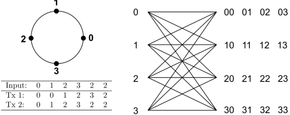
Let us consider, for example, the coding trellis of the full rate 2 bits/ channel uses STTCs with two transmit antennas. Fig 1.5 illustrates the 4-states space time code using 4-PSK modulation. STTCs code is represented by a trellis and pairs of symbols that are transmitted from the two antennas for every paths in the trellis. The indices of the symbols are used to present the transmitted symbols for each path (see Fig. 1.5).

0 1 2 3 1 2 3 00 01 02 03 10 11 12 13 20 21 22 23 30 31 32 33 0 Input: 0 1 2 3 2 2 Tx 1: 0 0 1 2 3 2 Tx 2: 0 1 2 3 2 2

1.5 Precoding technique

Precoding is a technique which exploits the channel state information at transmitter (CSIT) by processing signal before transmission. A basic precoding system structure which contains an encoder, a precoder and a decoder is shown in Fig 1.6. The encoder intakes data bits and performs necessary coding for error correction, and then maps the coded bits into vector symbols. The precoder processes these symbols before transmission according to different forms of channel state information. At the receive side, a decoder is considered to recover the bit streams.

Encoder Precoder _F Channel _H

₊

η

Transmitter

s

s

ˆ

CSIT

Figure 1.6: Precoding system structure.

1.5.1 Encoding structure

An encoder often consists of a channel coding and interleaving block and a symbol-mapping block. The encoding structure can be classified into two categories: spatial multiplexing and space time coding which are based on the symbol mapping block. The spatial multiplexing structure de-multiplexes the data bits to multiple independent bit streams. These bit streams are then mapped into vector symbols and are directly op-erated by a precoder, as shown in Fig 1.7. Since these streams are independent with individual signal to noise ratio (SNR), per-stream rate adaptation can be used for trans-mission.

Channel coding

&

Interleaving DEMUX Symbol Mapping

Symbol Mapping

Input

Output

For space-time coding structure, the output bits of the channel coding and interleaving block are directly mapped into symbols, and processed by a space-time encoder block (see Section 1.4). The vector symbols are then pre-multiplied by a precoding matrix, detailed in Fig1.8. Channel coding & Interleaving Space-Time Code Symbol Mapping Input Output

Figure 1.8: A space-time encoding structure.

1.5.2 Linear precoding structure

When the CSI is available at the transmitter, the precoder can optimize various criteria such as, for example, maximizing the output capacity [12], maximizing the mutual infor-mation [19], etc. However, it has also a general structure which is based on the singular value decomposition (SVD)

F = UΣV. (1.29)

In this structure, a linear precoder is considered as a combination of an input shaper and a multimode beamformer. The orthogonal beam directions are the left singular matrix U, where each column represents a beam direction (pattern). One should note that the matrix U contains all eigenvectors of the matrix FF∗_{, thus it is often referred to as}

eigen-beamforming. The matrix Σ controls the power allocation on each beam. These powers correspond to the squared singular values of Σ2_{. The right singular matrix V}

concerns with the rotation and scaling of the input symbols on each beam and hence is referred to as the input shaping matrix. The linear precoding structure is illustrated in Figure1.9. To conserve the total transmit power, the precoder must satisfy the condition

trace(FF∗) =E_s. (1.30)

where Esis the average transmit power. In other words, the sum of power over all beams

must be a constant. The individual beam power is different to each other according to the design criterion, the signal to noise ratio, and the CSIT.

σb . . .

×

×

V

U

Σ

Figure 1.9: A linear precoding structure.

1.5.3 Receiver structure

Let us denote s as the symbol vectors entering the precoder F at the transmitter, the received signal is then defined by

y = HFs + η, (1.31)

where η is a vector of additive white Gaussian noise. The received signal is then decoded to obtain an estimate of the transmitted codeword s. There are many detection meth-ods, depending on the performance of the system and the complexity of the detection. We present herein three representative methods: zero forcing (ZF), linear MMSE, and maximum-likelihood (ML).

Zero Forcing receiver

The zero-forcing receiver uses an inverse filter of the matrix HF to remove all of the interferences from other symbols. In the case of full rank square matrix HF (e.g. nT = nR), the inverse matrix (HF)−1exists and can be used to separate the received symbols.

When the number of transmit and receive antennas are not the same, the Moore–Penrose pseudo-inverse (HF)+_{is proposed to achieve a zero-forcing equalizer [20]. The estimation}

of the transmit symbols is then

ˆs = (HF)+y = s + (HF)+η, (1.32)

where (HF)+ _{denotes the pseudo-inverse matrix of HF, and is defined by (HF)}+ ₌

the power of the effective noise (HF)+_{η may be enhanced by the process of eliminating}

the symbol interference.

Minimum Mean-Squared Error receiver

In contrast to the ZF receiver, a linear minimum mean square error (MMSE) receiver is proposed to minimize the total effective noise. This receiver contains a weighting matrix W which is designed according to

min W E{∥ˆs − s∥ 2 } =min W E{∥(WHF − I)s + Wη∥ 2 }, (1.33)

where the expectation is taken over the input signal and noise distributions. For zero-mean signals with covariance equal to one, the optimum MMSE receiver is given as

W = (F∗H∗HF + nT

SNRI)−1F∗H∗, (1.34)

where nT is the number of transmit antennas, and SNR is the signal to noise ratio. Using

the MMSE criterion, the linear least-mean-squares estimation of transmitted symbols is defined by

ˆs = Wy. (1.35)

It is observed that when the ratio nT

SNR approaches to zero at high SNR, the ZF and

MMSE receivers are equivalent.

Maximum Likelihood receiver

The Maximum Likelihood (ML) detection provides a best performance in terms of bit-error-rate (BER) compared to other receivers. The estimation of the transmitted symbol s is defined by

ˆs = argmin

s

∥y − HFs∥2 (1.36)

The ML requires the receiver to consider all possible codewords s before making the decision and, therefore, can be computationally expensive. The complexity of the ML detection is exponentially proportional to the number of transmit antennas (proportion to MnT, where M is the size of the transmitted constellation). A new algorithm which

attains ML performances with significantly reduced complexity is presented in [21]. This scheme excludes unreliable candidate symbols in data streams and is based on the MMSE criterion to reduce the ML complexity. In order to decrease the computational complex-ity, the algorithm of sphere decoder can also be used to obtain an equivalent performance [22], [23].

Sphere Decoding Technique

The principle of sphere decoding technique is based on a bounded distance search among all possible points falling inside a sphere centered at the received point [24]. This concept is illustrated in Fig. 1.10, in which the received signal vector and the possible codewords are represented by a small and large circles, respectively. It is obvious that the overall complexity of the sphere decoding technique is lower than that of the original maximum-likelihood detection that implements a full search in all codewords space.

Figure 1.10: Principle of sphere decoding technique.

The search region in codewords space, i.e. the number of codewords close to the received signal, depends on the received signal-to-noise-ratio. Although worst case complexity is exponential, the expected complexity of the sphere decoding algorithms is polynomial

[25,26]. The fixed-complexity sphere decoder presented in [27] is one of the most

promis-ing approaches to not only enable quasi-ML decodpromis-ing accuracy but also to reduce the computational complexity. Another efficient closest point search algorithm, based on the Schnorr–Euchner variation of the Pohst method, is also presented in [28].

1.6 Conclusion

The primary purpose of this chapter is to review briefly the principal characteristics of MIMO wireless communications. Firstly, we presented the propagation over wireless channels and different types of diversity techniques. After that, a brief introduction of some MIMO techniques is referred. These techniques can be divided into three main cat-egories: spatial multiplexing, space-time coding, and precoding. The space-time coding technique is available when there is no channel state information at the transmitter while the precoding technique exploits the CSIT and processes signal before transmission. As the channel knowledge at the transmitter offers a high improvement in MIMO perfor-mance, the precoding technique becomes of great practical interest in wireless communi-cations. In the rest of this thesis, we investigate the performance and some extensions of the precoding technique based on the maximization of the minimum Euclidean distance in the received constellation.

MIMO linear precoding techniques

and nR receive antennas. There exist many methods to estimate MIMO channel at the

receiver [29,30], and we assume, in this thesis, that channel estimation provides a perfect channel state information at the receiver (CSIR). Through a feedback channel, channel state information is returned to the transmitter (CSIT), and a linear precoder can be designed according to this channel knowledge. Precoding design depends not only on the type of CSIT but also on the optimization criteria such as, for example, maximizing the received signal-to-noise ratio (SNR) [31], minimizing the mean square error (MSE) [32], or maximizing the minimum singular value of the channel matrix [33]. These solutions are all based on the singular value decomposition (SVD), which decouples MIMO channels into independent and parallel data-streams. Furthermore, they all perform a power allocation strategy on the MIMO eigen-subchannels. In other words, the data-streams at the transmitter are premultiplied by an eigen-diagonal precoding matrix. Hence, these precoders belong to an important set of linear precoding techniques named as diagonal precoders.

An alternative set of linear precoders is obviously the non-diagonal strategies. One of the most well-known non-diagonal precoding structure was invented independently by Tomlinson [34] and Harashima [35]. To optimize the Schur-convex functions of MSE for all channel substreams, a specific precoding matrix, which also leads to the non-diagonal structure, was proposed in [36]. Another non-non-diagonal precoder based on an

interesting criterion: maximizing the minimum Euclidean distance (max-dmin) between

two received data vectors, was firstly presented in [37]. It will be shown, in this chapter, that the precoder max-dmin proposes many interesting improvements compared to other

techniques. This precoder will be also investigated, in details, the performance in terms of bit error rate. Its extensions for high-order modulations will be shown in chapter 3, and for large MIMO systems in chapter 4.

2.1 Virtual transformation

+

Precoder

s

s

ˆ

CSIT CSIR Decoder

F

F

H

G

G

η

Figure 2.1: Virtual model of MIMO systems

Let us consider a MIMO channel with nR receive, nT transmit antennas over which we

want to transmit b independent data streams. Suppose there are a precoding matrix F at the transmitter and a decoding matrix G at the receiver, the basic system model can be expressed as

y = GHFs + Gη, (2.1)

where H is the nR×n_T channel matrix, F is the n_T×bprecoding matrix, G is the b × n_R decoding matrix, s is the b × 1 transmitted vector symbol, and η is the nR×1 additive noise vector. We should remark that b ≤ rank(H) ≤ min(nT, nR), so n_T and n_R can be larger than b. In the following sections, we assume

E[ss∗] =I_b, E[sη∗] =0and E[ηη∗] =R_η, (2.2) where Ib is the identity matrix of size b × b and Rη is the noise covariance matrix. Let

us define Es as the average transmit power. Thereafter, the precoding matrix F must

satisfy the power constraint

Step Method Fi Gi Hvi Rvi Noise whitening Rn=QΛQ∗ F1=InT G1=Λ -1_2Q∗ _H v1=G1HF1 Rv1=InR Channel diagonalization Hv1=AΣB∗ F2=B G2=A∗ Hv2=Σ Rv2=InR Dimensionality reduction F3= ( Ib 0) G3=(Ib 0) Hv=Σb Rnη=Ib

Table 2.1: Steps to obtain the diagonal MIMO system in the case of CSIT

If the channel state information (CSI) is perfectly known at both the transmitter and receiver, a diagonalized channel matrix and a whitened noise can be obtained. This operation is decomposed in three steps and is denoted as virtual transformation. The key of this method is illustrated in Fig. 2.1. Firstly, the precoding and decoding matrices are decomposed as F = FvFd and G = GdGv. Then, the new decompositions of two

matrices Fv and Gv into the product of three matrices are considered.

Fv=F₁F₂F₃ and G_v =G₁G₂G₃, (2.4)

where (Fi, Gi) perform the particular operations which are detailed in Tab. 2.1.

2.1.1 Noise whitening

Let us consider the eigenvalue decomposition of the noise covariance matrix

Rη=E[ηη∗] =QΛQ∗, (2.5)

where Q is a unitary matrix and Λ is a diagonal matrix. The goal of this step is to obtain the correlation matrix Rv1 =E[G1ηη∗G1∗] =G1QΛQ∗G1∗ equal to an identity matrix. The matrix G1 is therefore defined by

G1=Λ−1/2Q∗. (2.6)

The intermediate channel of this operation is given by

Hv1 =G1HF1, (2.7)

2.1.2 Channel diagonalization

The singular value decomposition (SVD) of the intermediate matrix Hv1 is used to di-agonalize the channel. Indeed, we have

Hv1 =AΣB

∗_{, (2.8)}

where A and B∗ _{are unitary matrices, and Σ is a diagonal matrix whose elements}

represent the square roots of all eigenvalues of the matrix Hv1H∗v1. One should note that these eigenvalues are real positive numbers and sorted in decreasing order. The number of non-null eigenvalues depends on the rank of the matrix Hv1

k = rank(Hv1) ≤min(nT, nR). (2.9)

The diagonal matrix Σ can be then expressed by these non-null eigenvalues Σ = ⎛ ⎜ ⎝ Σk 0 0 0 ⎞ ⎟ ⎠ (2.10) where the matrix Σk contains all of the non-null eigenvalues. To diagonalize the

inter-mediate channel matrix Hv1, the proposed solution is

F2=B and G₂=A∗. (2.11)

The second intermediate channel matrix Hv2 is then diagonal and defined by

Hv2 =G2Hv1F2=Σ. (2.12)

In addition, the correlation matrix Rv2 is given by

Rv2 =G2Rv1G∗2 =G2G∗2 =InR, (2.13) it is because G2 is a unitary matrix.

2.1.3 Dimensionality reduction

The diagonal form of the matrix Hv2 corresponds to the gains of each subchannels. It is noted that these diagonal elements are sorted in decreasing order. The goal of this operation is to obtain the dimension corresponding to the number of desired data-streams b. The matrices F3 and G3 are then defined by

F3= ⎛ ⎜ ⎝ Ib 0 ⎞ ⎟ ⎠ and G3= (Ib 0). (2.14)

These operations are only available if b ≤ k, so we consider the channel matrix such that b ≤ k = min(nT, nR). The resulting matrix is given by

Hv=G₃H_v2F₃=Σ_b, (2.15)

where Σb represents the b largest singular values of Hv1. The correlation matrix of the noise is also identity but the dimension is different

Rηv=Ib. (2.16)

2.1.4 Virtual channel representaion

The received signal in (2.1) is now re-expressed as

y = GdHvFds + Gdηv, (2.17)

where Hv=G_vHF_v is the b × b eigen-channel matrix, η_v=G_vη is the b × 1 virtual noise vector. Thanks to virtual transformation, the eigen-channel matrix Hv is diagonal and

defined by

Hv=diag(σ₁, ..., σ_b), (2.18)

where σi stands for every subchannel gain and is sorted by decreasing order. One should

note that the virtual precoding matrix Fv is orthonormal (e.g. F∗vFv =I), and the power constraint is then given by

The basic and the equivalent diagonal transmission systems are shown by the block diagram in Fig. 2.2. In these models, the input bit streams are firstly modulated to symbol streams are then passed through a linear precoder. The linear precoding matrix Fadd redundancy to the input symbol streams to improve the system performance. The output of the precoder is then sent to the channel H with the additive gaussian noise η. The decoding matrix G is used to remove any redundancy that has been introduced by the precoder. For the diagonal transmission model, the decoding matrix Gd will have

no influence on the performance and is consequently assumed to be an identity matrix if a maximum likelihood (ML) detection is considered at the receiver.

F

×

×

×

+

+

+

y

y

y

..

.

..

.

y

F

G

s

s

_ˆs

η

G

Figure 2.2: Block diagram of a MIMO system: basic model (a), diagonal transmission model (b).

The virtual precoding matrix Fd is used to optimize the criteria such as maximizing the

output capacity [12], maximizing the received signal-to-noise ratio (SNR) [31], minimiz-ing the mean square error (MSE) [32], maximizminimiz-ing the minimum sminimiz-ingular value of the channel matrix [33]. These precoders belong to the diagonal group. In other words, the precoding matrix Fdis diagonal and leads to power allocation on b parallel independent

data streams.

In the next sections, we present some of the traditional precoders and concentrate on a non-diagonal precoder which optimizes the minimum Euclidean distance between the received signals.

2.2 Existing precoders

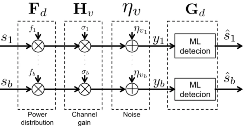
Due to the form of the precoder F, the precoding technique can be classified into two categories: diagonal and non-diagonal schemes. A precoder is called as diagonal if and only if the precoding and decoding matrices (Fd, Gd) in (2.17) are diagonal. When the receiver is based on a maximum likelihood detection, the decoding matrix Gd has

no influence on the performance and only the precoding matrix Fd=diag(f₁, f₂, ..., f_b) is considered in the optimization. The general principle of the diagonal precoder is illustrated in the Fig2.3. The problem becomes finding the power distribution expressed by the coefficients f2

i to optimize a particular criterion. We present, herein, some diagonal

precoders such as Beamforming, Water-Filling, Minimum Mean Square Error (MMSE), Quality of Service (QoS), and Equal Error (EE).

. . .

×

×

×

×

η

η

+

+

s

s

s

ˆ

ˆ

s

F

d

H

v

η

v

G

d

y

y

Figure 2.3: Diagonal precoding schema using maximum likelihood detection (ML) at the receiver.

2.2.1 Beamforming or max-SNR precoder

As its name implies, this precoder maximizes the signal to noise ratio (SNR) at the transmitter, and uses only the strongest virtual subchannel corresponding to the SNR σ2

1 [38, 39]. It concentrates all of the transmit power on the most favorable direction

represented by the singular vector associated with the maximum eigenvalue [31]. The expression of the received signal, in virtual representation, is then

y = √