Subproblem h-Conform Magnetodynamic Finite Element
Formulation for Accurate Model of Multiply Connected Thin
Regions
Vuong Q. Dang1,a, Patrick Dular1,2, Ruth V. Sabariego1, Laurent Kr¨ahenb¨uhl3and Christophe Geuzaine1 1University of Li`ege, Dept. of Electrical Engineering and Computer Science, ACE, B-4000 Li`ege, Belgium
2Fonds de la Recherche Scientifique - F.R.S.-FNRS, B-1000 Brussels, Belgium
3University of Lyon, Amp`ere (CNRS UMR5005), ´Ecole Centrale de Lyon, F-69134 ´Ecully Cedex, France
Received: date / Revised version: date
Abstract. A subproblem h-conform eddy current finite element method is proposed for correcting the inaccuracies inherent to thin shell models. Such models replace volume thin regions by surfaces but neglect border e↵ects in the vicinity of their edges and corners. The developed surface-to-volume correction problem is defined as a step of the multiple subproblems applied to a complete problem, consisting of inductors and magnetic or conducting regions, some of these being thin regions. The general case of multiply connected thin regions is considered.
1 Introduction
Thin shell (TS) finite element (FE) models [1], [2], [5], assume that the fields in the thin regions are approxi-mated by a priori 1-D analytical distributions along the shell thickness. In the frame of the FE method, their in-terior is thus not meshed and is rather extracted from the studied domain, being reduced to a zero-thickness double layer with interface conditions (ICs) linked to the inner analytical distributions. This means that corner and edge e↵ects are neglected.
To overcome these drawbacks, the subproblem method (SPM) for the h-conform FE formulation has been already developed in [3] for simply connected TS regions, propos-ing a surface-to-volume local correction. The method is herein extended to multiply connected TS regions, i.e. re-gions with holes, for both the associated surface model (alternative to the method in [5], [6]) and its volume cor-rection. The global currents flowing around the holes and their associated voltages are naturally coupled to the lo-cal quatities, via some cuts for magnetic slo-calar potential discontinuities at both TS and correction steps.
A reduced model (SP q) with the inductors alone is first considered before adding the TS FE (SP p), followed by the volume correction (SP k). From SP q to SP p, the solution q contributes to the surface sources (SSs) for the added TS, with TS ICs [2]. From SP p to SP k, SSs and volume sources (VSs) allow to suppress the TS and cut discontinuities and simultaneously add the actual volume
a E-mail: [email protected]
of the thin region, with its own cut discontinuity. Each SP requires a proper adapted mesh of its regions. The method is illustrated and validated on a practical problem.
2 Thin shell correction in the subproblem
method
2.1 Canonical magnetodynamic problem
A canonical magnetodynamic problem i, to be solved at step i of the SPM, is defined in a domain ⌦i, with
boundary @⌦i = i = h,i[ b,i. The eddy current
con-ducting part of ⌦iis denoted ⌦c,iand the non-conducting
region ⌦C
c,i, with ⌦i= ⌦c,i[ ⌦c,iC. Stranded inductors
be-long to ⌦C
c,i, whereas massive inductors belong to ⌦c,i.
The equations, material relations and boundary condi-tions (BCs) of the SPs i = q, p and k are
curl hi= ji, div bi= 0 , curl ei= @tbi (1a-b-c)
bi= µihi+ bs,i, ei= i 1ji+ es,i (2a-b)
n⇥ hi| h,i= jf,i, n· bi| b,i = bf,i (3a-b)
n⇥ ei| e,i⇢ b,i= kf,i (3c)
where hi is the magnetic field, bi is the magnetic flux
density, ei is the electric field, ji is the electric current
density, µi is the magnetic permeability, i is the electric
conductivity and n is the unit normal exterior to ⌦i. In
what follows the notation [·] i =| +
i | i expresses the
sides i+ and i ) in ⌦i, defining ICs. The fields bs,i and
es,i in (2a-b) are VSs that can be used for expressing
changes of permeability or conductivity respectively [13]. The fields jf,i, bf,iand kf,iin (3a-b-c) are SSs and
gen-erally equal zero with classical homogeneous BCs. Their discontinuities via ICs are also equal to zero for common continuous field traces n⇥hi, n·biand n⇥ei. If nonzero,
they define possible SSs that account for particular phe-nomena occuring in the idealized thin region between i+
and i [13]. This is the case when some field traces in SP p are forced to be discontinuous, whereas their continuity must be recovered via a SP k, which is done via a SS in SP k fixing the opposite of the trace discontinuity solution of SP p.
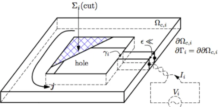
Fig. 1. 3D plate with a source of electromotive force 2.2 From SP q to SP p - inductor alone to TS model
The TS model for the hi-formulation requires an
un-known discontinuity hd,i through the TS t,i of the
tan-gential component ht,i = (n⇥ hi)⇥ n of hi [2], i.e.
[ht,i] t,i= hd,i or [n⇥ hi] t,i= n⇥ hd,i (4)
with hd,ifixed to zero along the TS border to prevent any
current to flow through it. In order to explicitly express the discontinuity, field hi is written on both sides of t,i
as
hi| +
t,i= hc,i+ hd,i, hi| t,i= hc,i (5)
with hc,iits continuous component; (5) can be also applied
to the tangential components ht,i, ht,c,i and ht,d,i.
SSs for SP p are to be defined via BCs and ICs of impedance-type BCs (IBC) given by the TS model [2] combined with contributions from SP q. There is no thin region in SP q, but in order to get a relative constraint between SP q and SP p via the corresponding ICs with
t= ±t = q±= p± = ts,q± = ts,p± and nt= n for the
TS, one has to imagine that a thin region appears in SP q. One gets for SP q and SP p [2], [3]
[n⇥ eq] q = n⇥ eq| q+ n⇥ eq| q = 0 (6) [n⇥ e] p= [n⇥ eq] p+ [n⇥ ep] p= µ @t(2hc+ hd) (7) n⇥ ep| + p = 1 2 ⇥ µ @t(2hc+ hd) + 1 hd⇤ n⇥ eq| + p (8) = i 1tanh( di i 2 ), i= 1 + j i , i= r 2 ! iµi (9)
where di is the local TS thickness, i is the skin depth in
the TS, ! = 2⇡f , f is the frequency, j is the imaginary unit and @t⌘ j!. The discontinuity [n ⇥ eq] p in (7) does
not need any correction because solution SP q presents no such discontinuitiy, i.e. [n⇥ eq] q = [n⇥ eq] p= 0.
2.3 From SP p to SP k - TS to volume model
The obtained TS solution in SP p is then corrected by SP k that overcomes the TS assumptions [2]. The SPM o↵ers the tools to implement such as refinement, thanks to simultaneous SSs and VSs. A fine volume mesh of the shell is now required and is extended to its neighborhood without including the other regions of previous SPs. This allows to focus on the fineness of the mesh only in the shell. SP k has to suppress the TS representation via SSs opposed to TS ICs, in parallel to VSs in the added volume shell [3] that accounts for volume change of µp and p in
SP p to µk and k in SP k (with µp= µ0, µk= µr,volume, p= 0 and k = volume). This correction is usually
lim-ited to the neighborhood of the shell, which permits to benefit from a reduction of the extension of the associated mesh [3]. The VSs for SP k are [3], [12], [13]
bs,k= (µk µp)(hq+ hp) (10)
es,k= (eq+ ep) (11)
3 Finite element weak formulations
3.1 h- formulation with source and reaction magnetic fields
The weak hi- iformulation is obtained from the weak
form of Faraday’s law (1c) [13]. The magnetic field hi is
split into two parts, i.e.
hi= hs,i+ hr,i (12)
where hs,i is a source magnetic field due to the fixed
current density js,i such that curl hs,i = js,i, and hr,i
is the reaction magnetic field. In non-conducting regions ⌦C
c,i, field hr,i is defined via a scalar potential i, i.e.
hr,i= grad i. Potential i in a multiply connected ⌦c,iC
is multivalued (Fig. 1) and is made singlevalued via the definition of cuts through each hole of ⌦c,i [7], [9]. The
constraints associated with the cut and the discontinuity of the tangential component of the magnetic field across the thin structures are expressed in Section 3.2. The weak forms for SP q and SP p are
@t(µqhq, h0q)⌦q+ @t(µqhs,q, h 0 q)⌦q+hn ⇥ eq, h 0 qi e,q+ h[n ⇥ eq] q, h 0 qi q= 0 , 8h 0 q 2 Fq,h1 (⌦q) (13) @t(µphp, h0p)⌦p+hn ⇥ ep, h 0 pi e,p +h[n ⇥ ep] p, h 0 pi p= 0 , 8h 0 p2 Fp,h1 (⌦p) (14) where F1
i,h (⌦i) in (13) and (14) is a curl-conform function
on ⌦i and containing the basis functions for hi (coupled
to i) as well as for the test function h0i; (· , ·)⌦i and <
· , · > i respectively, denote a volume intergal in ⌦i and a
surface intergal on i of the product of their vector field
arguments. The surface integral term on e,i accounts for
natural BCs of type (3c), usually zero. The termh[n ⇥ ep] p, h
0
pi p in (14) is used to weakly
express the electric field TS IC proper to the TS model [2], i.e h[n ⇥ ep] p, h 0 pi p=h[n ⇥ ep] p, h 0 c+ h0di p =h[n ⇥ ep] p, h 0 ci p+h[n ⇥ ep] p, h 0 di p. (15)
Splitting test function h0pinto continous and discontinuous
parts, i.e. h0c and h0d, with h0d null on the negative side of
TS p, like in (5), equation (15) becomes [2]
h[n ⇥ ep] p, h 0 pi p=h[n ⇥ ep] p, h 0 ci p+ hn ⇥ ep| p+, h0di p+. (16)
The trace discontinuity term h[n ⇥ ep] p, h
0 ci p in (16) is given by (7), i.e. h[n ⇥ ep] p, h 0 ci p =h[n ⇥ e] p, h 0 ci p =hµ @t(2hc+ hd), h0ci p. (17)
The termhn ⇥ ep| p+, h0di p+ in (16) is given by (8),
sup-pressing n⇥ eq| p+ of SP q and simultaneously adding the
actual TS BC. Therefore, the term hn ⇥ ep| p+, h0di p+ is
a SS that is naturally expressed via the weak formulation of SP q (13), i.e. hn ⇥ eq| + p, h 0 di + p = (µq@ths,q, h 0 d)⌦q+ (µq@thq, h 0 d)⌦q. (18) The volume integrals in (18) are also limited to a single layer of FEs touching +
p = +q = ts+, because they
in-volve only the trace n⇥ h0d| +
p. At the discrete level, the
source hq, initially in the mesh of SP q, has to be projected
in the mesh of SP p via a projectiong method [3], [13]. Then the actual volume SP k corrects the inaccurate TS SP p solution via VSs (10) and (11).
In addition, the surface integral hn ⇥ ep, h0pi e,p in
(14) can be extended to a global condition defining a voltage Vi [4], with h0p = ci = grad qi in ⌦Cc,p with
n⇥ ci = n⇥ grad qi on @⌦c,p (ci is the current
ba-sis function) made simply connected by cut ⌃i (Figs. 1
and 2). Potential qi is fixed to 1 on one side of the cut
and to 0 on the other side. The continuous transition of qi
between both these value can be implemented in a tran-sition layer in ⌦C
c,p adjacent to side ’+’ (Figs. 1 and 2),
which reduces the suport of qi and ci. One gets [4]
hn ⇥ ep, cii@⌦c,p = I @ i qiep.dl = Z gi ep.dl = Vi (19)
where gi is a path connecting two real or imaginary
elec-trodes of the thin region. The weak form of SP k is @t(µkhk, h0k)⌦k+ ( 1 k curl hk, curl h0k)⌦c,k+ @t(bs,k, h 0 k)⌦k +(es,k, curl h0k)⌦k+h[n ⇥ ek] k, h 0 ki k+hn ⇥ ek, h 0 ki e,k = 0,8h0k2 Fk,h1 (⌦k) . (20)
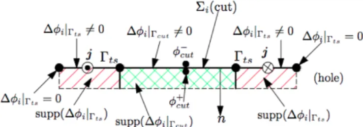
3.2 Field discontinuities for multiply connected TS regions
With the TS model, a volume shell initially in ⌦c,i
is extracted from ⌦i and then considered with the
dou-ble layer TS surface ts,i [2]. In addition to the electric
field IC weakly defined in (14), the TS model requires a magnetic field discontinuity [hi] ts,i = hd,i strongly
defined in F1
i,h (⌦i) via an IC on both sides of the TS
via (5). This can be formulated via a TS discontinuity of i, i.e. [ i] ts,i = i| ts,i = d,i| ts,i (Fig. 2), with
i| +
ts,i= c,i| ts,i+ d,i| ts,i and i| ts,i = c,i| ts,i. The
discontinuity d,iis constant on each cut and can be
writ-ten as
i= c,i+ d,i( d,i= d| cut,i = [ d,i]cut,i) (21)
[ i]cut,i= i| +
cut,i i| cut,i= d,i| cut,i = Ii (22)
where Ii is the global current flowing around the cut [4].
Discontinuities d,i| ts,iand d,i| cut,ihave to be matched
at the TS-cuts intersections.
Fig. 2. Section of a 3D plate with a hole, with the associated cut and transition layer (supp) for i.
3.3 Discretization of the reaction magnetic field At the discrete level, the use of edge FEs [2], [8] to interpolate curl-conform fields, such as the magnetic filed hi, first gives facilities in defining currents. Indeed, the
circulation of such a field along closed path, also being the flux of its curl and consequently the current, is directly obtained from coefficients of the interpolation, in this case those associated with the edges of the path [11].
The magnetic field hi (12) in formulations (13), (14)
and (20) is thus discretized by edge FEs, generating the function space 2 S1
i(⌦i) defined on a mesh of ⌦i, i.e.,
hi=
X
e2E(⌦i)
he,ise,i, 8hi2 Si1(⌦i) (23)
where E(⌦i) is the set of edges of ⌦i, se,iis the edge basis
function associated with edge e and he,i is the circulation
of hi along the edge e. Now, characterization (23) can be
transformed in order to give explicitly the basis functions of the considered discrete space for F1
hi, i(⌦i) with the
essential constraint, i.e., hr,i= grad iusing the results
of [4], [10]. One has hi=
X
e2E(⌦c,i) E(@⌦c,i)
he,ise,i+ X n2N(⌦C c,i) c,n,ivc,n,i + X n2N( ts,i) d,itd,n,i+ Ici X n2N( cut,i) cd,n,i (24)
where E(⌦c,i) E(@⌦c,i) are the sets of inner edges of the
mesh of ⌦c,i, without including the edges on its boundary,
N (⌦C
c,i) is the sets of nodes of the mesh of ⌦c,iC [ @⌦c,iC,
N ( ts,i) is the sets of nodes of the mesh of ts,i and
N ( cut,i) is the sets of nodes of the mesh of cut,imaking
⌦C
c simply connected [7]. Coefficients Ici represent
circu-lations of hi along well-defined paths given by (22). The
functions td,n,iand cd,n,ican be respectively expressed in
the thin regions and the cuts as [2]
td,n,i= 8 > > > > > > > > < > > > > > > > > : X {n, m} 2 E(⌦C c,i) n2 N( ts,i) m62 N( ts,i) m2 Nts,i+
se,{n,m}in supp( i| ts,i)
0 otherwise cd,n,i= 8 > > > > > > > > < > > > > > > > > : X {n, m} 2 E(⌦C c,i) n2 N( cut,i) m62 N( cut,i) m2 N+ cut,i se,{n,m}in supp( i| cut,i) 0 otherwise where m2 N+
ts,i and m2 Ncut,i+ are the sets of nodes of
the transition layers supp( i| ts,i) and supp( i| cut,i),
respectively (Fig. 2).
3.4 TS correction - VSs in the actual volume shell and SSs for suppressing the TS representation
Changes of material properties from µp and p in SP
p to µk and k in SP k, that occur in the volume shell,
are taken into account in (20) via the volume integrals (es,k, curl h0k)⌦k and @t(bs,k, h
0
k)⌦k. The VS es,k in (11)
is to be obtained from the still undetermined electric fields eq and ep. Therefore, the field epis unknown in any ⌦c,pC .
These determinations require to solve an electric problem defined by the Faraday and electric conservation equa-tions [13].
Simultaneously to the VSs in (20), SSs related to ICs [2], [3] compensate the TS and cut discontinuities, i.e,
d,p| ts,p and d,p| cut,p, and [n⇥ ep] ts,p to suppress the
TS representation via SSs opposed to ICs, i.e. hd,k =
hd,pand d,k= d,p, and [n⇥ek] ts,k = [n⇥ep] ts,p.
The involed trace [n⇥ ep] ts,k is naturally expressed via
the other integrals in (14), i.e., h[n ⇥ ek] ts,k, h
0
ki ts,k =
h[n⇥ep] ts,k, h
0
ki ts,k. At the discrete level, this integral
is limited to the layer of FEs on both sides ts,k of TS,
because it involves only the associated trace n⇥ h0k| ts,k.
The source hp, with its discontinuity hd,p, has also to be
transferred from the mesh of TS SP p to the mesh of SP k.
3.5 Projections of solutions between meshes
Some parts of previous solutions serve as sources in a subdomain ⌦s,p ⇢ ⌦p of the current SP p, for example
from SP q to SP p. At the discrete level, this means that the source quantities hq have to be expressed in the mesh
of SP p, while initially given in the mesh of SP q. This can be done via a projection method [14] of its curl limited to ⌦s,p, i.e.
(curl hq,p proj, curl h0)⌦s,p = (curl hq, curl h
0) ⌦s,p,
8h02 Fp1(⌦s,p) (25)
where F1
p(⌦s,p) is a gauged curl-conform function space
for the p-projected source hq,p proj (the projection of hq
on mesh p) and the test function h0. Directly projecting hq instead of its curl would give numerical inaccuracies
when evaluating its curl.
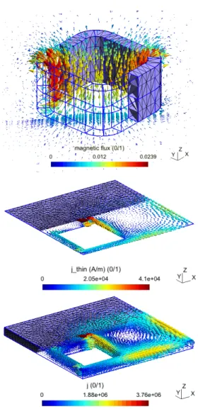
4 Application
The 3D test problem is based on TEAM problem 7: an inductor placed above a thin plate with a hole (Fig. 3) (µr,plate = 1, plate = 35.26 MS/m). A SP scheme
con-sidering three steps is developed. A first FE SP q with the stranded inductor alone is solved on a simplified mesh without any thin regions (Fig. 4, top). Then a SP p is solved with the added thin region via a TS FE model (Fig. 4, middle). At last, a SP k replaces the TS FEs with the actual volume FEs covering the actual plates with an adequate refine mesh (Fig. 4, bottom). The TS error on jp
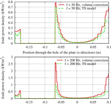
locally reaches 43% (Fig. 4, middle), with plate thickness d = 19 mm and frequency f = 200 Hz (skin depth = 6 mm). The inacuracy on the Joule power loss densities of TS SP p is pointed out by the importance of the cor-rection SP k (Figs. 5 and 6). It reaches several tens of percents along the plate borders and near the plate ends for some critical parameters: e.g., 28% (Fig. 5, top) and 32% (Fig. 6, top), with f = 50 Hz and = 11.98 mm in both case, or 53% (Fig. 5, bottom) and 61% (Fig. 6, bottom), with f = 200 Hz and = 6 mm in both cases. The errors particularly decrease with a smalller thickness (d = 2 mm), being lower than 15% (Fig. 6), with f = 200 Hz and = 6 mm. Significant errors on the Joule losses and the global currents flowing around the hole for TS SP p are shown in Tables 1 and 2. For d = 19 mm and f = 200 Hz, the TS error is 13.5% for the global current and 42% for the Joule loss (reduced to 26% for f = 50 Hz). For d = 2 mm and f = 200 Hz, it is respectively reduced to 1% and 6% (4% for f = 50 Hz).
5 Conclusions
The SPM allows to accurately correct any TS solu-tion. In particular, accurate corrections of eddy current and power loss densities are obtained at the edges and cor-ners of multiply connected thin regions. All the steps of the method for TS FE have been presented and validated
Fig. 3. Geometry of TEAM problem 7: inductor and conduct-ing plate with a hole (all dimensions are in mm).
Table 1. Joule losses in the plate
Thickness Frequency Thin Shell Volume Error d (mm) f (Hz) Pthin(W) Pvol(W) (%)
2 50 14.45 13.82 4.36 19 50 5.86 7.95 26.18
2 200 50.44 47.33 6.44 19 200 8.88 15.19 41.51
Table 2. Global currents flowing around the plate hole
Thickness Frequency Thin Shell Volume Error d (mm) f (Hz) Ithin(A) Ivol (A) (%)
2 50 94,5 93.5 1.1 19 50 173.3 199.8 13.2
2 200 190.4 186.5 1.8 19 200 179.3 206.3 14
by coupling SPs via the SPM with the h-formulation. Spe-cially, it has been sucessfully applied to the TEAM prob-lem 7.
6 Acknowledgment
This work was supported by the Belgium Sciency Pol-icy (IAP 7/21)
References
1. L. Kr¨ahenb¨uhl and D. Muller, “Thin layers in electrical engineering. Examples of shell models in analyzing
eddy-Fig. 4. TEAM problem 7: magnetic flux density bq (in a cut plane) generated by a stranded inductor (top), TS eddy current density jp (middle) and its volume correction jk (bottom) (d = 19 mm, f = 200 Hz).
currents by boundary and finite element methods,” IEEE Trans. Magn., vol. 29, no. 2, pp. 1450–1455, 1993.
2. C. Geuzaine, P. Dular, and W. Legros, “Dual formulations for the modeling of thin electromagnetic shells using edge elements,” IEEE Trans. Magn., vol. 36, no. 4, pp. 799–802, 2000.
3. Vuong Q. Dang, P. Dular, R. V. Sabariego, L. Kr¨ahenb¨uhl and C. Geuzaine, “Subproblem Approach for Thin Shell Dual Finite Element Formulations,” IEEE Trans. Magn., vol. 48, no. 2, pp. 407–410, 2012.
4. P. Dular and W. Legros, “Coupling of Local and Global Quantities in Various Finite Element Formulations and its Application to Electrostatics, Magnetostatics and Magne-todynamics,” IEEE Trans. Magn., vol. 34, no. 5, pp. 3078 –3081, 1998.
5. C. Gu´erin and G. Meunier, “3-D Magnetic Scalar Potential Finite Element Formulation for Conducting Shells Coupled With an External Circuit,” IEEE Trans. Magn., vol. 48, no. 2, pp. 323–326, 2012.
6. T. Le-Duc, C. Gu´erin, O. Chadebec, and J.-M. Guichon “A New Integral Formulation for Eddy Current Computation
0 0.1 0.2 0.3 0.4 0.5 0.6 0.7 0.8 0.9 -0.15 -0.1 -0.05 0 0.05 0.1
Joule power density (kW/m
2 )
Position along the hole of the plate (x-direction) (m) f = 50 Hz, volume correction f = 50 Hz, TS model 0 0.2 0.4 0.6 0.8 1 1.2 1.4 1.6 -0.15 -0.1 -0.05 0 0.05 0.1
Joule power density (kW/m
2 )
Position along the hole of the plate (x-direction) (m) f = 200 Hz, volume correction f = 200 Hz, TS model
Fig. 5. Joule power loss density for TS model and volume correction along hole and plate borders (d = 19 mm).
0 0.1 0.2 0.3 0.4 0.5 0.6 0.7 0.8 -0.15 -0.1 -0.05 0 0.05 0.1
Joule power density (kW/m
2 )
Position through the hole of the plate (x-direction) (m) f = 50 Hz, volume correction f = 50 Hz, TS model 0 0.5 1 1.5 2 2.5 3 -0.15 -0.1 -0.05 0 0.05 0.1
Joule power density (kW/m
2 )
Position through the hole of the plate (x-direction) (m) f = 200 Hz, volume correction f = 200 Hz, TS model
Fig. 6. Joule power loss density for TS model and volume correction through the hole (d = 19 mm).
in Thin Conductive Shells,” IEEE Trans. Magn., vol. 48, no. 2, pp. 427–430, 2012.
7. A. Bossavit, “Magnetostatic problems in multiply con-nected regions: some properties of the curl operator,” IEE
Proc. vol. 135, no. 3, pp. 179–187, 1988.
8. A. Bossavit, “A rationale for edge-elements in 3D fields computations,” IEEE Trans. Magn., vol. 24, no. 1, pp. 74– 79, 1988. 0 1 2 3 4 5 -0.15 -0.1 -0.05 0 0.05 0.1
Joule power density (kW/m
2 )
Position along the hole of the plate (x-direction) (m) f = 50 Hz, volume correction f = 50 Hz, TS model f = 200 Hz, volume correction f = 200 Hz, TS model 0 1 2 3 4 5 -0.15 -0.1 -0.05 0 0.05 0.1
Joule power density (kW/m
2 )
Position through the hole of the plate (x-direction) (m) f = 50 Hz, volume correction f = 50 Hz, TS model f = 200 Hz, volume correction f = 200 Hz, TS model
Fig. 7. Joule power loss density for TS model and volume correction along hole and plate borders (top) and through the hole (bottom) (d = 2 mm).
9. D. Rodger and N. Atkinson, “3D eddy currents in multiply connected thin sheet conductors,” IEEE Trans. Magn., vol. 23, no. 5, pp. 3047–3049, 1987.
10. P. Dular, J.Y. Hody and A. Nicolet and A.Genon and A. Gennon and W. Legros, “Mixed finite elements associated with a collection of tetrahedra, hexahedra and prism,” IEEE Trans. Magn., vol. 30, no. 5, pp. 2980-2983, 1994.
11. P. Dular, F. Henrotte and A. Gennon and W. Legros, “A generlized source magnetic field calculation method for in-ductors of any shape,” IEEE Trans. Magn., vol. 33, no. 2, pp. 1398-1401, 1997.
12. P. Dular, R. V. Sabariego and L. Kr¨ahenb¨uhl, “Mag-netic Model Refinement via a Perturbation Finite Element Method - From 1-D to 3-D,” COMPEL, vol. 28, no. 4, pp. 974-988, 2009.
13. P. Dular and R. V. Sabariego, “A perturbation method for computing field distortions due to conductive regions with h-conform magnetodynamic finite element formulations,” IEEE Trans. Magn., vol. 43, no. 4, pp. 1293-1296, 2007. 14. C. Geuzaine, B. Meys, F. Henrotte, P. Dular and
W. Legros, “A Galerkin projection method for mixed fi-nite elements,” IEEE Trans. Magn., Vol. 35, No. 3, pp. 1438-1441, 1999.