Application and processing of geophysical images for mapping faults

Application and processing of geophysical images for mapping faults

Donat Demanet*, François Renardy*, Eric Pirard** and Denis Jongmans*

B-4000 Liège, Belgium

**MICA, Geomaterials Characterisation Laboratory, Liège University, Bât. D2, Avenue des Tilleuls 45,B-4000 Liège, Belgium

[email protected], [email protected], [email protected], [email protected]

Abstract

Location of active faults in superficial quaternary sediments is a field of increasing interest. In this paper, we applied two imaging methods (electrical and seismic refraction tomography) to this aim. Both methods are successful but provide relatively smooth images which are prone to the subjectivity of the interpreter. Image analysis techniques (watershed divide line on gradient images) are applied to the tomography results to add objectivity to the interpretation. Application to synthetic cases as well as to actual images showed that the developed algorithm can be of great aid.

Keywords

Electrical Tomography, Seismic Refraction Tomography, Inversion, Image analysis, Faults.

Introduction

Even when a geomorphological expression of a fault is present in the topography, the fault trace is often difficult to locate accurately. Non-destructive geophysical prospecting techniques may then be applied in order to map the fault trace with accuracy in the superficial sediments. During these last few years, a large number of high-resolution seismic reflection surveys have been conducted (see e.g., Williams et al., 1995; Palmer et al., 1997; Van Arsdale et al., 1998) to provide information on Quaternary fault geometry and timing in different areas. For very shallow investigation, ground-penetrating radar (GPR) has been recently applied by Cai et al. (1996) in the San Francisco Bay region. At the border of Nevada and California, Shields et al. (1998) employed several geophysical techniques (seismic reflection, magnetics and electromagnetics) to locate the extension of the Parhump Valley fault zone. This paper describes the application of two geophysical prospecting techniques to image fault zones: electrical tomography and seismic refraction tomography. This work is part of the results of a geophysical campaign performed in the Roer Graben area as a reconnaissance tool before trenching, and which included several geophysical prospecting methods. The aim of this investigation was in the first place to determine the exact position of the active fault, in order to constrain the best emplacement of a later trench. An additional objective was to image the fault zone at shallow depth, allowing both a comparison with trench data, and a downward extrapolation of these direct observations. In order to constrain a

non-subjective interpretation of such images, image analysis techniques have been applied on the geophysical results. Additionally, synthetic models representing resistivity anomalies along a faulted section were used to check the reliability of the image processing method.

Electrical tomography

Electrical Tomography is a 2D imaging technique showing the variation of the ground resistivity along a section. It is based on the same principles as such other classical electrical methods like sounding or profiling. A controlled current (I) is injected into the ground with two electrodes, while measuring the potential (V) between two other electrodes. The resistance is calculated using Ohm's law. The material parameter resistivity (ρ), which is the inverse of electrical conductivity (σ) is related to the resistance via a geometrical factor. To build an electrical image of the ground (a 2D section of resistivity), numerous measurements are carried out for various combinations of potential and current electrodes. The Wenner configuration (constant offset between electrodes) has been used. The first step in the data interpretation consists in building a pseudo-section obtained by plotting the apparent resistivity versus the depth (proportional to the offset between electrodes) for each midpoint of a given electrode configuration. This representation leads to a qualitative image where neither the resistivities nor the depths are correct.

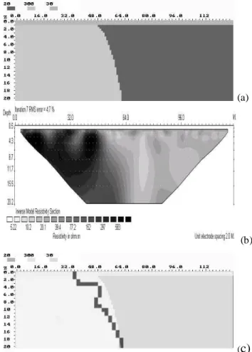
It is necessary to inverse the pseudo-section in order to determine a vertical resistivity section as a function of a true depth. The inversion of the data is carried out according to an iterative process which aims at minimizing the difference between the measured pseudo-section and a calculated pseudo-section based on a model. This model is updated after each iteration until reaching an acceptable agreement between measured and calculated data or until no further improvement is possible. The data are processed with the algorithm proposed by Loke & Barker (1996) implemented in the RES2DINV software. Figure 1 shows the results of a survey performed at Jülich (Germany) across the escarpment of the Peel fault. The aim of this investigation is to determine the exact position of the fault as well as to image the fault zone at shallow depth. This work has been realised in collaboration with the Geological Survey of North-Westphalia and the University of Köln. The field measurements were performed with ABEM devices: Electrode Selector ES-464 and Terrameter 300C. Four cables with an amount of 64 connectors were extended along the profile. With a 2 meters constant electrode offset, this provides a total length of 126 meters.

Fig. 1 Electrical tomography (after inversion) across the escarpment of a presumed active fault - Jülich.

Figure 1 very clearly highlights a sharp lateral variation of resistivity at about 60 m. The top of the escarpment is more resistive than the bottom. The main problem with interpreting pseudocolor visualisations is the low-pass filtering generated by the inversion process associated to the subjectivity of the human's eye. In order to improve the interpretation of such results and the location of the true anomaly, it was decided to tentatively use image analysis.

Fig. 2. Automatic delineation (dark line) of major resistivity anomalies using a conditional watershed divide

line algorithm.

The aim of this latter is to mark the strongest gradient of resistivity separating regions of homogeneous appearance. The principles of image processing are detailed in the last section. Results of the automatic anomaly location in Jülich are presented in Figure 2.

Another important point is the accuracy of the determined characteristics of the fault (location and dip). Several synthetic models have been created according to the results presented in Figure 1. A model with a thin horizontal low-resistivity layer overlying a vertical or dipping fault was created (Fig. 3a). The layers on both sides of the fault were given different combinations of resistivity values (300Ωm /100Ωm /20Ωm) so as to study the influence of the contrast on the interpretation. The pseudo-section corresponding to the model was then inversed using RES2DINV. Finally, image processing was performed on this inversed model in order to locate the highest gradient of resistivity. The comparison between the model, the inversed section and the result of the image analysis process for the dipping fault case is presented in Figure 3. Comparison with the result of the same computations on the vertical fault case (not illustrated) shows that it is possible to discriminate the two types of fault.

(a)

(b)

(c)

Fig. 3. Model with an oblique fault (a), the resistivity image obtained after inversion (b) and the automatic delineation

of the anomaly after image processing (c)

Seismic refraction tomography

The test site was selected based on a preliminary paleoseismological study in the Roer graben near the city of Bree (NE of Belgium). In the framework of this project, several geophysical measurements were carried out across

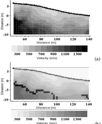
the escarpment of a presumed active fault in order to locate and to image the fault zone. The results combined with the dig of a 80 m long and 3.5 m deep trench revealed two faults separated by 25 m (Demanet et al ,1999). 300 500 700 900 1100 1300 60 80 100 120 140 -10 0 5 -5 Elevation (m) Distance (m) Velocity (m/s)

_(a)

_(b)

Fig. 4. Seismic refraction tomography image from the Bree fault escarpment (a) and the location of anomalies obtained from the conditional watershed divide line (b).

The first step in the refraction tomography survey consists of measuring first-arrival times between sources and receivers located along a profile crossing the fault escarpment. Combining travel-times from a number of sources and receivers at different positions along the profile, one can determine the P-wave velocity distribution on a two-dimensional section. Various numerical inversion schemes have been proposed for image reconstruction (see Ivansson, 1986). In this study, we have used the Simultaneous Iterative Reconstruction Technique (SIRT) developed by Gilbert (1972). In this iterative method, which is presented in detail by Krajewski et al. (1989), a first guess of the solution is assumed and the theoretical travel-times are computed for each ray. The residuals between calculated and observed times are then used to correct the velocity values along the ray path, giving a new image. The iterative procedure is stopped when some criteria are met; for instance when the rms (root mean square) of the residual travel-times is assessed as low enough. Our software, developed in-house, uses curved rays computed from the gradient of the traveltime on the whole grid. The acquisition configuration was 96 m long with one receiver every two meters. The source was a hammer with a shot-point at each geophone position. Data were stacked at least 6 times for each source. The starting model of the inversion process was based on

the results of a classical seismic refraction profile along the fault escarpment. The inversion process was stopped after 10 iterations. The stopping criteria were the rms and the standard error of both the residual travel-times and the velocity variations between two iterations. Results of the inversion are presented in Figure 4.

Two sharp dipping anomalies are situated around 70 and 95 m exhibiting a stair-shaped section and correlating very well with the preliminary geophysical study and the trench observations.

The image processing technique developed for the analysis of electrical tomography sections was kept for this profile and revealed the anomalies presented in Figure 4(b) after thresholding of low gradient transitions.

Image processing

In order to fit with the requirements of the image processing algorithms, geophysical data were converted into 256 grey levels (8 bits) bitmap format. The electrical tomographies were typically 60x20 pixels whereas seismic images had a resolution of 48x20 pixels. All routines used for image processing were developed within Micromorph (Beucher, 1995).

The processing algorithm was defined, keeping in mind that the major aim was to localize transitions between more or less homogeneous domains. The first step therefore consisted in building a correct gradient image. Because nothing was known a priori about the shape of the gradient, it was decided to check the adequacy of the gradient computation on resistivity tomographies simulated from simple geometries (Figure 3).

The chosen gradient computation was a supremum of directional morphological gradients (linear dilation minus linear erosion) in the four major directions of the octagonal grid. The size of the gradient is obviously limited by the poor resolution of electrical tomographies and was most often set to two, meaning in practice a gradient over a linear segment of five pixels. It is to be noted that median filtering had been included in the image inversion process, thereby precluding the need for any further smoothing of the original image before computing the gradient. Figure 5 displays the result of the gradient computation.

Fig. 5. Gradient image from the electrical tomography taken in Jülich (figure 1)

Major discontinuities in the resistivity image appear as crest lines after computing the gradient image. They are too numerous and too erratic to be extracted by direct grey level skeletonization and a conditional watershed approach seems to be more appropriate.

The watershed divide line as defined by Beucher and Meyer (1992) is a dam builded on the grey level image, considered as a relief, in order to avoid mixing of different sources. These sources can be true local minima in the image or any kind of user defined marker (see applications of the swamping technique in Serra, 1995).

In the present case, if "geological units" are to be identified in the image, they should correspond to homogeneous responses in resistivity or in other words, to very low values of the gradient. Therefore, the detection of the markers of the different geological units is based on a simple threshold of the gradient intensities. The typical threshold for eliminating too large gradients was set at values close to 5 to 10 gradient units (less than 5% of the 8 bits dynamic).

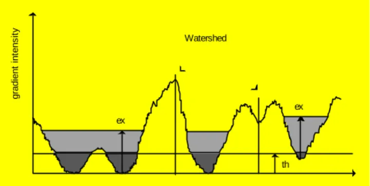
In order to improve the detection of strong discontinuities, a second step of marker growing is often desired. The original low gradient markers are therefore allowed to propagate within their neighbourhood as long as they stay within a given gradient intensity tolerance (typically 10 to 20 units). The result is such that low gradient markers that are only separated by a crest below the tolerance limit will be allowed to fusion into a unique marker, thereby avoiding an additional and poorly significant watershed divide line in the final image. Figure 6 schematically illustrates the principle of segmentation. ex ex th gradient intensity Watershed

Fig. 6. Section in a gradient image illustrating the principles of minimum gradient detection (th = threshold level; ex = tolerance) and watershed divide line marking.

The final watershed is computed from the gradient image using the low and homogeneous gradient regions as markers for the propagation. As can be seen from Figure 3, comparison with the original geometry of synthetic images gives a reasonable agreement. For real cases such as Figure 2 and Figure 5 the results are in accordance with visual interpretation. However, when contrast is diminishing, the result may become unstable with respect to the operators choice for the threshold and tolerance parameters calling for the need of a more precise gradient computation.

The evolution of divide lines with respect to tolerance and threshold values could be used as a method to classify the discontinuities in various classes ranging from extremely probable to possible.

CONCLUSIONS

This paper presented the application of two imaging methods to map active faults: electrical and seismic refraction

tomography. Both were successful in the location of the faults. As the resulting images are relatively smooth and can be interpreted with some subjectivity, image analysis techniques have been applied to locate more precisely and objectively the faults. The developed algorithm is still at an early stage but proved to be helpful. Possible enhancements could be: use of higher dynamic range (16 bit) images, computation of gradients normalized with respect to distance, hierarchical classification of anomalies. The study of the robustness with respect to operator choice of the parameters has also to be considered.

ACKNOWLEDGEMENTS

Part of this project was realized under the contract ENV4-CT97-0578 funded by the European Commission. We also wish to thank the Royal Observatory of Belgium for its contribution.

REFERENCES

BEUCHER, S. 1995. Micromorph, un logiciel d'apprentissage de la Morphologie Mathématique, Journées d'études

INRP/CNAM "Images numériques dans l'enseignement des sciences", 77-80.

BEUCHER, S., MEYER, F. 1992. The morphological approach to segmentation : the watershed transformation. In : Dougherty, E. (Ed.) Mathematical Morphology in Image Processing, Marcel Dekker, N.Y., 433-481.

CAI, J., MCMECHAN, A. & FISHER, M.A.,1996. Application of ground penetrating radar to investigation of near-surface fault properties in the San Francisco bay region. Bull.

Seismol. Soc. Am., 86, 1459-1470.

DEMANET, D., RENARDY, F.,VANNESTE, K.,JONGMANS, D., CAMELBEECK, T. & MEGHRAOUI, M., 1999. The use of geophysical prospecting for imaging active faults in the Roer graben, Belgium. Geophysics, submitted.

DOCHERTY, P.,1992. Solving for the thickness and velocity of the weathering layer using 2-D refraction tomography.

Geophysics, 57, 1307-1318.

GILBERT, P.,1972. Iterative methods for the three-dimensionnal reconstruction of an object from projections.

Journal of Theoritical Biology, 36, 105-117.

IVANSSON, S. 1987. Crosshole transmission tomography. In: NOLET, G.(ed.) Seismic Tomography, D. Reidel Publishing Company, Dordrecht, 159-188.

LOKE, M.H.& BARKER, R.D., 1996. Rapid least-squares inversion of apparent resistivity pseudo-sections by quasi-Newton method. Geophysical Prospecting, 44, 131-152. SERRA, J. 1995. Morphological image segmentation, Acta

Stereologica, 14/2, 99-111.

WILLIAMS, R. A., LUZIETTI, E.A. & CARVER, D.L.,1995. High-resolution imaging of Quaternary faulting on the Crittenden County fault zone, New Madrid seismic zone, northeastern Arkansas. Seismological Research Letters, 66, 42-57.