HAL Id: hal-02329000
https://hal.archives-ouvertes.fr/hal-02329000v2
Submitted on 7 Feb 2020
HAL is a multi-disciplinary open access
archive for the deposit and dissemination of
sci-entific research documents, whether they are
pub-lished or not. The documents may come from
teaching and research institutions in France or
abroad, or from public or private research centers.
L’archive ouverte pluridisciplinaire HAL, est
destinée au dépôt et à la diffusion de documents
scientifiques de niveau recherche, publiés ou non,
émanant des établissements d’enseignement et de
recherche français ou étrangers, des laboratoires
publics ou privés.
A Recurrent Variational Autoencoder for Speech
Enhancement
Simon Leglaive, Xavier Alameda-Pineda, Laurent Girin, Radu Horaud
To cite this version:
Simon Leglaive, Xavier Alameda-Pineda, Laurent Girin, Radu Horaud.
A Recurrent
Varia-tional Autoencoder for Speech Enhancement. ICASSP 2020 - IEEE InternaVaria-tional Conference on
Acoustics, Speech and Signal Processing, IEEE, May 2020, Barcelone (virtual), Spain.
pp.1-7,
�10.1109/ICASSP40776.2020.9053164�. �hal-02329000v2�
A RECURRENT VARIATIONAL AUTOENCODER FOR SPEECH ENHANCEMENT
Simon Leglaive
1,2Xavier Alameda-Pineda
2Laurent Girin
2,3Radu Horaud
21
CentraleSupélec, IETR, France
2Inria Grenoble Rhône-Alpes, France
3Univ. Grenoble Alpes, Grenoble INP, GIPSA-lab, France
ABSTRACT
This paper presents a generative approach to speech enhancement based on a recurrent variational autoencoder (RVAE). The deep gen-erative speech model is trained using clean speech signals only, and it is combined with a nonnegative matrix factorization noise model for speech enhancement. We propose a variational expectation-maximization algorithm where the encoder of the RVAE is fine-tuned at test time, to approximate the distribution of the latent vari-ables given the noisy speech observations. Compared with previous approaches based on feed-forward fully-connected architectures, the proposed recurrent deep generative speech model induces a poste-rior temporal dynamic over the latent variables, which is shown to improve the speech enhancement results.
Index Terms— Speech enhancement, recurrent variational au-toencoders, nonnegative matrix factorization, variational inference.
1. INTRODUCTION
Speech enhancement is an important problem in audio signal pro-cessing [1]. The objective is to recover a clean speech signal from a noisy mixture signal. In this work, we focus on single-channel (i.e. single-microphone) speech enhancement.
Discriminative approaches based on deep neural networks have been extensively used for speech enhancement. They try to estimate a clean speech spectrogram or a time-frequency mask from a noisy speech spectrogram, see e.g. [2, 3, 4, 5, 6]. Recently, deep gener-ative speech models based on variational autoencoders (VAEs) [7] have been investigated for single-channel [8, 9, 10, 11] and multi-channel speech enhancement [12, 13, 14]. A pre-trained deep gen-erative speech model is combined with a nonnegative matrix fac-torization (NMF) [15] noise model whose parameters are estimated at test time, from the observation of the noisy mixture signal only. Compared with discriminative approaches, these generative methods do not require pairs of clean and noisy speech signal for training. This setting was referred to as “semi-supervised source separation” in previous works [16, 17, 18], which should not be confused with the supervised/unsupervised terminology of machine learning.
To the best of our knowledge, the aforementioned works on VAE-based deep generative models for speech enhancement have only considered an independent modeling of the speech time frames, through the use of feed-forward and fully connected architectures. In this work, we propose a recurrent VAE (RVAE) for modeling the speech signal. The generative model is a special case of the one proposed in [19], but the inference model for training is different. At test time, we develop a variational expectation-maximization al-gorithm (VEM) [20] to perform speech enhancement. The encoder Xavier Alameda-Pineda acknowledges the French National Research Agency (ANR) for funding the ML3RI project. This work has been partially supported by MIAI @ Grenoble Alpes, (ANR-19-P3IA-0003).
of the RVAE is fine-tuned to approximate the posterior distribution of the latent variables, given the noisy speech observations. This model induces a posterior temporal dynamic over the latent vari-ables, which is further propagated to the speech estimate. Experi-mental results show that this approach outperforms its feed-forward and fully-connected counterpart.
2. DEEP GENERATIVE SPEECH MODEL
2.1. Definition
Let s = {sn ∈ CF}N−1n=0 denote a sequence of short-time Fourier transform (STFT) speech time frames, and z = {zn ∈ RL}N−1n=0 a corresponding sequence of latent random vectors. We define the fol-lowing hierarchical generative speech model independently for all time frames n∈ {0, ..., N − 1}:
sn∣ z ∼ Nc(0, diag {vs,n(z)}) , with zn i.i.d
∼ N (0, I) , (1) and where vs,n(z) ∈ RF+ will be defined by means of a decoder neu-ral network. N denotes the multivariate Gaussian distribution for a real-valued random vector andNcdenotes the multivariate complex
proper Gaussian distribution [21]. Multiple choices are possible to define the neural network corresponding to vs,n(z), which will lead
to different probabilistic graphical models represented in Fig. 1. FFNN generative speech model vs,n(z) = ϕFFNNdec (zn; θdec)
where ϕFFNNdec (⋅ ; θdec) ∶ RL ↦ RF+ denotes a feed-forward fully-connected neural network (FFNN) of parameters θdec. Such an
architecture was used in [8, 9, 10, 11, 12, 13, 14]. As represented in Fig. 1a, this model results in the following factorization of the complete-data likelihood:
p(s, z; θdec) = ∏N−1n=0 p(sn∣zn; θdec)p(zn). (2)
Note that in this case, the speech STFT time frames are not only conditionally independent, but also marginally independent, i.e. p(s; θdec) = ∏N−1n=0 p(sn; θdec).
RNN generative speech model vs,n(z) = ϕRNNdec,n(z0∶n; θdec)
where ϕRNNdec,n(⋅ ; θdec) ∶ RL×(n+1)↦ RF+ denotes the output at time
frame n of a recurrent neural network (RNN), taking as input the sequence of latent random vectors z0∶n = {zn′ ∈ R
L}n n′=0. As
represented in Fig. 1b, we have the following factorization of the complete-data likelihood:
p(s, z; θdec) = ∏ N−1
n=0 p(sn∣z0∶n; θdec)p(zn). (3)
Note that for this RNN-based model, the speech STFT time frames are still conditionally independent, but not marginally independent. BRNN generative speech model vs,n(z) = ϕBRNNdec,n(z; θdec) where
ϕBRNN
s0 z0 s1 z1 s2 z2 (a) FFNN s0 z0 s1 z1 s2 z2 (b) RNN s0 z0 s1 z1 s2 z2 (c) BRNN Fig. 1: Probabilistic graphical models for N= 3.
a bidirectional RNN (BRNN) taking as input the complete sequence of latent random vectors z. As represented in Fig. 1c, we end up with the following factorization of the complete-data likelihood:
p(s, z; θdec) = ∏ N−1
n=0 p(sn∣z; θdec)p(zn). (4)
As for the RNN-based model, the speech STFT time frames are con-ditionally independent but not marginally.
Note that for avoiding cluttered notations, the variance vs,n(z)
in the generative speech model (1) is not made explicitly dependent on the decoder network parameters θdec, but it clearly is.
2.2. Training
We would like to estimate the decoder parameters θdec in the
max-imum likelihood sense, i.e. by maximizing∑Ii=1ln p(s(i); θdec),
where{s(i) ∈ CF×N}Ii=1is a training dataset consisting of I i.i.d sequences of N STFT speech time frames. In the following, be-cause it simplifies the presentation, we simply omit the sum over the I sequences and the associated subscript(i).
Due to the non-linear relationship between s and z, the marginal likelihood p(s; θdec) = ∫ p(s∣z;θdec)p(z)dz is analytically
in-tractable, and it cannot be straightforwardly optimized. We therefore resort to the framework of variational autoencoders [7] for parame-ters estimation, which builds upon stochastic fixed-form variational inference [22, 23, 24, 25, 26].
This latter methodology first introduces a variational distribu-tion q(z∣s; θenc) (or inference model) parametrized by θenc, which
is an approximation of the true intractable posterior distribution p(z∣s; θdec). For any variational distribution, we have the following
decomposition of log-marginal likelihood:
ln p(s; θdec) = Ls(θenc, θdec) + DKL(q(z∣s; θenc) ∥ p(z∣s; θdec)),
(5) whereLs(θenc, θdec) is the variational free energy (VFE) (also
re-ferred to as the evidence lower bound) defined by:
Ls(θenc, θdec) = Eq(z∣s;θenc)[ln p(s, z; θdec) − ln q(z∣s; θenc)]
= Eq(z∣s;θenc)[ln p(s∣z; θdec)] − DKL(q(z∣s; θenc) ∥ p(z)), (6)
and DKL(q ∥ p) = Eq[ln q − ln p] is the Kullback-Leibler (KL)
divergence. As the latter is always non-negative, we see from (5) that the VFE is a lower bound of the intractable log-marginal likeli-hood. Moreover, we see that it is tight if and only if q(z∣s; θenc) =
p(z∣s; θdec). Therefore, our objective is now to maximize the VFE
with respect to (w.r.t) both θenc and θdec. But in order to fully
de-fine the VFE in (6), we have to dede-fine the form of the variational distribution q(z∣s; θenc).
Using the chain rule for joint distributions, the posterior distri-bution of the latent vectors can be exactly expressed as follows:
p(z∣s; θdec) = ∏ N−1
n=0 p(zn∣z0∶n−1, s; θdec), (7)
where we considered p(z0∣z−1, s; θdec) = p(z0∣s; θdec). The
varia-tional distribution q(z∣s; θenc) is naturally also expressed as:
q(z∣s; θenc) = ∏ N−1
n=0 q(zn∣z0∶n−1, s; θenc). (8)
In this work, q(zn∣z0∶n−1, s; θenc) denotes to the probability density
function (pdf) of the following Gaussian inference model:
zn∣z0∶n−1, s∼ N (µz,n(z0∶n−1, s), diag {vz,n(z0∶n−1, s)}), (9)
where{µz,n, vz,n}(z0∶n−1, s) ∈ RL× RL+will be defined by means of an encoder neural network.
Inference model for the BRNN generative speech model For the BRNN generative speech model, the parameters of the variational distribution in (9) are defined by
{µz,n, vz,n}(z0∶n−1, s) = ϕBRNNenc,n(z0∶n−1, s; θenc), (10)
where ϕBRNNenc,n(⋅, ⋅ ; θenc) ∶ RL×n× CF×N ↦ RL× RL+ denotes the
output at time frame n of a neural network whose parameters are denoted by θenc. It is composed of:
1. “Prediction block”: a causal recurrent block processing z0∶n−1; 2. “Observation block”: a bidirectional recurrent block processing
the complete sequence of STFT speech time frames s;
3. “Update block”: a feed-forward fully-connected block process-ing the outputs at time-frame n of the two previous blocks. If we want to sample from q(z∣s; θenc) in (8), we have to sample
recursively each zn, starting from n= 0 up to N − 1. Interestingly,
the posterior is formed by running forward over the latent vectors, and both forward and backward over the input sequence of STFT speech time-frames. In other words, the latent vector at a given time frame is inferred by taking into account not only the latent vectors at the previous time steps, but also all the speech STFT frames at the current, past and future time steps. The anti-causal relationships were not taken into account in the RVAE model [19].
Inference model for the RNN generative speech model Using the fact that znis conditionally independent of all other nodes in Fig. 1b
given its Markov blanket (defined as the set of parents, children and co-parents of that node) [27], (7) can be simplified as:
p(zn∣z0∶n−1, s; θdec) = p(zn∣z0∶n−1, sn∶N−1; θdec), (11)
where sn∶N−1 = {sn′ ∈ CF}N−1n′=n. This conditional independence
also applies to the variational distribution in (9), whose parameters are now given by:
{µz,n, vz,n}(z0∶n−1, s) = ϕenc,nRNN(z0∶n−1, sn∶N−1; θenc), (12)
where ϕRNNenc,n(⋅, ⋅ ; θenc) ∶ RL×n× CF×(N−n)↦ RL× RL+ denotes the same neural network as for the BRNN-based model, except that the observation block is not a bidirectional recurrent block anymore, but an anti-causal recurrent one. The full approximate posterior is now formed by running forward over the latent vectors, and backward over the input sequence of STFT speech time-frames.
Inference model for the FFNN generative speech model For the same reason as before, by studying the Markov blanket of zn in
Fig. 1a, the dependencies in (7) can be simplified as follows:
This simplification also applies to the variational distribution in (9), whose parameters are now given by:
{µz,n, vz,n}(z0∶n−1, s) = ϕFFNNenc (sn; θenc), (14)
where ϕFFNNenc (⋅ ; θenc) ∶ CF ↦ RL× RL+ denotes the output of an
FFNN. Such an architecture was used in [8, 9, 10, 11, 12, 13, 14]. This is the only case where, from the approximate posterior, we can sample all latent vectors in parallel for all time frames, without fur-ther approximation.
Here also, the mean and variance vectors in the inference model (9) are not made explicitly dependent on the encoder network pa-rameters θenc, but they clearly are.
Variational free energy Given the generative model (1) and the general inference model (9), we can develop the VFE defined in (6) as follows (derivation details are provided in Appendix A.1):
Ls(θenc, θdec) c = −F∑−1 f=0 N−1 ∑ n=0Eq(z∣s;θenc)[dIS(∣sf n∣ 2 , vs,f n(z)) ] +1 2 L−1 ∑ l=0 N−1 ∑ n=0Eq(z0∶n−1∣s;θenc)[ ln (vz,ln(z0∶n−1 , s)) − µ2 z,ln(z0∶n−1, s) − vz,ln(z0∶n−1, s)], (15)
where= denotes equality up to an additive constant w.r.t θc enc and
θdec, dIS(a, b) = a/b − ln(a/b) − 1 is the Itakura-Saito (IS)
di-vergence [15], sf n ∈ C and vs,f n(z) ∈ R+ denote respectively
the f -th entries of sn and vs,n(z), and µz,ln(z0∶n−1, s) ∈ R
and vz,ln(z0∶n−1, s) ∈ R+ denote respectively the l-th entry of
µz,n(z0∶n−1, s) and vz,n(z0∶n−1, s).
The expectations in (15) are analytically intractable, so we com-pute unbiased Monte Carlo estimates using a set{z(r)}Rr=1of i.i.d. realizations drawn from q(z∣s; θenc). For that purpose, we use the
“reparametrization trick” introduced in [7]. The obtained objective function is differentiable w.r.t to both θdec and θenc, and it can be
optimized using gradient-ascent-based algorithms. Finally, we re-call that in the final expression of the VFE, there should actually be an additional sum over the I i.i.d. sequences in the training dataset {s(i)}I
i=1. For stochastic or mini-batch optimization algorithms, we would only consider a subset of these training sequences for each update of the model parameters.
3. SPEECH ENHANCEMENT: MODEL AND ALGORITHM
3.1. Speech, noise and mixture model
The deep generative clean speech model along with its parameters learning procedure were defined in the previous section. For speech enhancement, we now consider a Gaussian noise model based on an NMF parametrization of the variance [15]. Independently for all time frames n∈ {0, ..., N − 1}, we have:
bn∼ Nc(0, diag{vb,n}), (16)
where vb,n= (WbHb)∶,nwith Wb∈ RF×K+ and Hb∈ RK×N+ . The noisy mixture signal is modeled as xn= √gnsn+bn, where
gn∈ R+is a gain parameter scaling the level of the speech signal at
each time frame [9]. We further consider the independence of the speech and noise signals so that the likelihood is defined by:
xn∣ z ∼ Nc(0, diag{vx,n(z)}) , (17)
where vx,n(z) = gnvs,n(z) + vb,n.
3.2. Speech enhancement algorithm
We consider that the speech model parameters θdecwhich have been
learned during the training stage are fixed, so we omit them in the rest of this section. We now need to estimate the remaining model parameters φ= {g = [g0, ..., gN−1]⊺, Wb, Hb} from the
observa-tion of the noisy mixture signal x = {xn ∈ CF}N−1n=0. However,
very similarly as for the training stage (see Section 2.2), the marginal likelihood p(x; φ) is intractable, and we resort again to variational inference. The VFE at test time is defined by:
Lx(θenc, φ) = Eq(z∣x;θenc)[ln p(x∣z; φ)]−DKL(q(z∣x; θenc) ∥ p(z)).
(18) Following a VEM algorithm [20], we will maximize this criterion alternatively w.r.t θencat the E-step, and φ at the M-step. Note that
here also, we haveLx(θenc, φ) ≤ ln p(x; φ) with equality if and
only if q(z∣x; θenc) = p(z∣x; φ).
Variational E-Step with fine-tuned encoder We consider a fixed-form variational inference strategy, reusing the inference model learned during the training stage. More precisely, the variational distribution q(z∣x; θenc) is defined exactly as q(z∣s; θenc) in (9) and
(8) except that s is replaced with x. Remember that the mean and variance vectors µz,n(⋅, ⋅) and vz,n(⋅, ⋅) in (9) correspond to the
VAE encoder network, whose parameters θencwere estimated along
with the parameters θdec of the generative speech model. During
the training stage, this encoder network took clean speech signals as input. It is now fine-tuned with a noisy speech signal as input. For that purpose, we maximizeLx(θenc, φ) w.r.t θenconly, with fixed φ.
This criterion takes the exact same form as (15) except that∣sf n∣2is
replaced with∣xf n∣2where xf n ∈ C denotes the f-th entry of xn,
s is replaced with x, and vs,f n(z) is replaced with vx,f n(z), the
f -th entry of vx,n(z) which was defined along with (17). Exactly
as in Section 2.2, intractable expectations are replaced with a Monte Carlo estimate and the VFE is maximized w.r.t. θenc by means of
gradient-based optimization techniques. In summary, we use the framework of VAEs [7] both at training for estimating θdecand θenc
from clean speech signals, and at testing for fine-tuning θencfrom
the noisy speech signal, and with θdecfixed. The idea of refitting the
encoder was also proposed in [28] in a different context.
Point-estimate E-Step In the experiments, we will compare this variational E-step with an alternative proposed in [29], which con-sists in relying only on a point estimate of the latent variables. In our framework, this approach can be understood as assuming that the approximate posterior q(z∣x; θenc) is a dirac delta function
cen-tered at the maximum a posteriori estimate z⋆. Maximization of p(z∣x; φ) ∝ p(x∣z; φ)p(z) w.r.t z can be achieved by means of gradient-based techniques, where backpropagation is used to com-pute the gradient w.r.t. the input of the generative decoder network. M-Step For both the VEM algorithm and the point-estimate al-ternative, the M-Step consists in maximizingLx(θenc, φ) w.r.t. φ
under a non-negativity constraint and with θencfixed. Replacing
in-tractable expectations with Monte Carlo estimates, the M-step can be recast as minimizing the following criterion [9]:
C(φ) = ∑R r=1∑ F−1 f=0 ∑ N−1 n=0 dIS(∣xf n∣2, vx,f n(z(r))) , (19)
where vx,f n(z(r)) implicitly depends on φ. For the VEM
algo-rithm,{z(r)}Rr=1is a set of i.i.d. sequences drawn from q(z∣x; θenc)
using the current value of the parameters θenc. For the point
esti-mate approach, R= 1 and z(1)corresponds to the maximum a pos-teriori estimate. This optimization problem can be tackled using a
majorize-minimize approach [30], which leads to the multiplicative update rules derived in [9] using the methodology proposed in [31] (these updates are recalled in Appendix A.2).
Speech reconstruction Given the estimated model parameters, we want to compute the posterior mean of the speech coefficients:
ˆ sf n= Ep(sf n∣xf n;φ)[sf n] = Ep(z∣x;φ)[ √g nvs,f n(z) vx,f n(z) ] x f n. (20)
In practice, the speech estimate is actually given by the scaled co-efficients √gnˆsf n. Note that (20) corresponds to a Wiener-like
fil-tering, averaged over all possible realizations of the latent variables according to their posterior distribution. As before, this expectation is intractable, but we approximate it by a Monte Carlo estimate us-ing samples drawn from q(z∣x; θenc) for the VEM algorithm. For
the point-estimate approach, p(z∣x; φ) is approximated by a dirac delta function centered at the maximum a posteriori.
In the case of the RNN- and BRNN-based generative speech models (see Section 2.1), it is important to remember that sam-pling from q(z∣x; θenc) is actually done recursively, by sampling
q(zn∣z0∶n−1, x; θenc) from n = 0 to N − 1 (see Section 2.2).
There-fore, there is a posterior temporal dynamic that will be propagated from the latent vectors to the estimated speech signal, through the ex-pectation in the Wiener-like filtering of (20). This temporal dynamic is expected to be beneficial compared with the FFNN generative speech model, where the speech estimate is built independently for all time frames.
4. EXPERIMENTS
Dataset The deep generative speech models are trained using around 25 hours of clean speech data, from the "si_tr_s" subset of the Wall Street Journal (WSJ0) dataset [32]. Early stopping with a patience of 20 epochs is performed using the subset "si_dt_05" (around 2 hours of speech). We removed the trailing and leading silences for each utterance. For testing, we used around 1.5 hours of noisy speech, corresponding to 651 synthetic mixtures. The clean speech signals are taken from the "si_et_05" subset of WSJ0 (unseen speakers), and the noise signals from the "verification" subset of the QUT-NOISE dataset [33]. Each mixture is created by uniformly sampling a noise type among {"café", "home", "street", "car"} and a signal-to-noise ratio (SNR) among {-5, 0, 5} dB. The intensity of each signal for creating a mixture at a given SNR is computed using the ITU-R BS.1770-4 protocol [34]. Note that an SNR computed with this protocol is here 2.5 dB lower (in average) than with a simple sum of the squared signal coefficients. Finally, all signals have a 16 kHz-sampling rate, and the STFT is computed using a 64-ms sine window (i.e. F= 513) with 75%-overlap.
Network architecture and training parameters All details re-garding the encoder and decoder network architectures and their training procedure are provided in Appendix A.3.
Speech enhancement parameters The dimension of the latent space for the deep generative speech model is fixed to L= 16. The rank of the NMF-based noise model is fixed to K = 8. Wb and
Hbare randomly initialized (with a fixed seed to ensure fair
com-parisons), and g is initialized with an all-ones vector. For computing (19), we fix the number of samples to R= 1, which is also the case for building the Monte Carlo estimate of (20). The VEM algorithm and its "point estimate" alternative (referred to as PEEM) are run for 500 iterations. We used Adam [35] with a step size of 10−2for
Algorithm Model SI-SDR (dB) PESQ ESTOI MCEM [9] FFNN 5.4± 0.4 2.22± 0.04 0.60 ± 0.01 PEEM FFNN 4.4± 0.4 2.21± 0.04 0.58 ± 0.01 RNN 5.8± 0.5 2.33± 0.04 0.63 ± 0.01 BRNN 5.4± 0.5 2.30± 0.04 0.62 ± 0.01 VEM FFNN 4.4± 0.4 1.93± 0.05 0.53 ± 0.01 RNN 6.8± 0.4 2.33± 0.04 0.67 ± 0.01 BRNN 6.9± 0.5 2.35± 0.04 0.67 ± 0.01 noisy mixture -2.6± 0.5 1.82± 0.03 0.49 ± 0.01 oracle Wiener filtering 12.1± 0.3 3.13± 0.02 0.88 ± 0.01
Table 1: Median results and confidence intervals.
the gradient-based iterative optimization technique involved at the E-step. For the FFNN deep generative speech model, it was found that an insufficient number of gradient steps had a strong negative impact on the results, so it was fixed to 10. For the (B)RNN model, this choice had a much lesser impact so it was fixed to 1, thus limit-ing the computational burden.
Results We compare the performance of the VEM and PEEM al-gorithms for the three types of deep generative speech model. For the FFNN model only, we also compare with the Monte Carlo EM (MCEM) algorithm proposed in [9] (which cannot be straightfor-wardly adapted to the (B)RNN model). The enhanced speech quality is evaluated in terms of scale-invariant signal-to-distortion ratio (SI-SDR) in dB [36], perceptual evaluation of speech quality (PESQ) measure (between -0.5 and 4.5) [37] and extended short-time objec-tive intelligibility (ESTOI) measure (between 0 and 1) [38]. For all measures, the higher the better. The median results for all SNRs along with their confidence interval are presented in Table 1. Best results are in black-color-bold font, while gray-color-bold font indi-cates results that are not significantly different. As a reference, we also provide the results obtained with the noisy mixture signal as the speech estimate, and with oracle Wiener filtering. Note that oracle results are here particularly low, which shows the difficulty of the dataset. Oracle SI-SDR is for instance 7 dB lower than the one in [9]. Therefore, the VEM and PEEM results should not be directly compared with the MCEM results provided in [9], but only with the ones provided here.
From Table 1, we can draw the following conclusions: First, we observe that for the FFNN model, the VEM algorithm performs poorly. In this setting, the performance measures actually strongly decrease after the first 50-to-100 iterations of the algorithm. We did not observe this behavior for the (B)RNN model. We argue that the posterior temporal dynamic over the latent variables helps the VEM algorithm finding a satisfactory estimate of the overparametrized posterior model q(z∣x; θenc). Second, the superiority of the RNN
model over the FFNN one is confirmed for all algorithms in this comparison. However, the bidirectional model (BRNN) does not perform significantly better than the unidirectional one. Third, the VEM algorithm outperforms the PEEM one, which shows the inter-est of using the full (approximate) posterior distribution of the latent variables and not only the maximum-a-posteriori point estimate for estimating the noise and mixture model parameters. Audio examples and code are available online [39].
5. CONCLUSION
In this work, we proposed a recurrent deep generative speech model and a variational EM algorithm for speech enhancement. We showed that introducing a temporal dynamic is clearly beneficial in terms of speech enhancement. Future works include developing a Markov chain EM algorithm to measure the quality of the proposed varia-tional approximation of the intractable true posterior distribution.
6. REFERENCES
[1] P. C. Loizou, Speech enhancement: theory and practice, CRC press, 2007.
[2] Y. Xu, J. Du, L.-R. Dai, and C.-H. Lee, “A regression approach to speech enhancement based on deep neural networks,” IEEE Trans. Audio, Speech, Language Process., vol. 23, no. 1, pp. 7–19, 2015. [3] F. Weninger, H. Erdogan, S. Watanabe, E. Vincent, J. Le Roux, J. R.
Hershey, and B. Schuller, “Speech enhancement with LSTM recurrent neural networks and its application to noise-robust ASR,” in Proc. Int. Conf. Latent Variable Analysis and Signal Separation (LVA/ICA), 2015, pp. 91–99.
[4] D. Wang and J. Chen, “Supervised speech separation based on deep learning: An overview,” IEEE Trans. Audio, Speech, Language Pro-cess., vol. 26, no. 10, pp. 1702–1726, 2018.
[5] X. Li, S. Leglaive, L. Girin, and R. Horaud, “Audio-noise power spec-tral density estimation using long short-term memory,” IEEE Signal Process. Letters, vol. 26, no. 6, pp. 918–922, 2019.
[6] X. Li and R. Horaud, “Multichannel speech enhancement based on time-frequency masking using subband long short-term memory,” in Proc. IEEE Workshop Applicat. Signal Process. Audio Acoust. (WAS-PAA), 2019.
[7] D. P. Kingma and M. Welling, “Auto-encoding variational Bayes,” in Proc. Int. Conf. Learning Representations (ICLR), 2014.
[8] Y. Bando, M. Mimura, K. Itoyama, K. Yoshii, and T. Kawahara, “Sta-tistical speech enhancement based on probabilistic integration of vari-ational autoencoder and non-negative matrix factorization,” in Proc. IEEE Int. Conf. Acoust., Speech, Signal Process. (ICASSP), 2018, pp. 716–720.
[9] S. Leglaive, L. Girin, and R. Horaud, “A variance modeling framework based on variational autoencoders for speech enhancement,” in Proc. IEEE Int. Workshop Machine Learning Signal Process. (MLSP), 2018, pp. 1–6.
[10] S. Leglaive, U. ¸Sim¸sekli, A. Liutkus, L. Girin, and R. Horaud, “Speech enhancement with variational autoencoders and alpha-stable distribu-tions,” in Proc. IEEE Int. Conf. Acoust., Speech, Signal Process. (ICASSP), 2019, pp. 541–545.
[11] M. Pariente, A. Deleforge, and E. Vincent, “A statistically principled and computationally efficient approach to speech enhancement using variational autoencoders,” in Proc. Interspeech, 2019.
[12] K. Sekiguchi, Y. Bando, K. Yoshii, and T. Kawahara, “Bayesian multi-channel speech enhancement with a deep speech prior,” in Proc. Asia-Pacific Signal and Information Processing Association Annual Summit and Conference (APSIPA ASC), 2018, pp. 1233–1239.
[13] S. Leglaive, L. Girin, and R. Horaud, “Semi-supervised multichannel speech enhancement with variational autoencoders and non-negative matrix factorization,” in Proc. IEEE Int. Conf. Acoust., Speech, Signal Process. (ICASSP), 2019, pp. 101–105.
[14] M. Fontaine, A. A. Nugraha, R. Badeau, K. Yoshii, and A. Liutkus, “Cauchy multichannel speech enhancement with a deep speech prior,” in Proc. European Signal Processing Conference (EUSIPCO), 2019. [15] C. Févotte, N. Bertin, and J.-L. Durrieu, “Nonnegative matrix
factor-ization with the Itakura-Saito divergence: With application to music analysis,” Neural Computation, vol. 21, no. 3, pp. 793–830, 2009. [16] P. Smaragdis, B. Raj, and M. Shashanka, “Supervised and
semi-supervised separation of sounds from single-channel mixtures,” in Proc. Int. Conf. Indep. Component Analysis and Signal Separation, 2007, pp. 414–421.
[17] G. J. Mysore and P. Smaragdis, “A non-negative approach to semi-supervised separation of speech from noise with the use of temporal dynamics,” in Proc. IEEE Int. Conf. Acoust., Speech, Signal Process. (ICASSP), 2011, pp. 17–20.
[18] N. Mohammadiha, P. Smaragdis, and A. Leijon, “Supervised and unsu-pervised speech enhancement using nonnegative matrix factorization,” IEEE Trans. Audio, Speech, Language Process., vol. 21, no. 10, pp. 2140–2151, 2013.
[19] J. Chung, K. Kastner, L. Dinh, K. Goel, A. C. Courville, and Y. Bengio, “A recurrent latent variable model for sequential data,” in Proc. Adv. Neural Information Process. Syst. (NIPS), 2015, pp. 2980–2988.
[20] R. M. Neal and G. E. Hinton, “A view of the EM algorithm that justi-fies incremental, sparse, and other variants,” in Learning in Graphical Models, M. I. Jordan, Ed., pp. 355–368. MIT Press, 1999.
[21] F. D. Neeser and J. L. Massey, “Proper complex random processes with applications to information theory,” IEEE Trans. Information Theory, vol. 39, no. 4, pp. 1293–1302, 1993.
[22] M. I. Jordan, Z. Ghahramani, T. S. Jaakkola, and L. K. Saul, “An introduction to variational methods for graphical models,” Machine Learning, vol. 37, no. 2, pp. 183–233, 1999.
[23] A. Honkela, T. Raiko, M. Kuusela, M. Tornio, and J. Karhunen, “Ap-proximate Riemannian conjugate gradient learning for fixed-form vari-ational Bayes,” Journal of Machine Learning Research, vol. 11, no. Nov., pp. 3235–3268, 2010.
[24] T. Salimans and D. A. Knowles, “Fixed-form variational posterior ap-proximation through stochastic linear regression,” Bayesian Analysis, vol. 8, no. 4, pp. 837–882, 2013.
[25] M. D. Hoffman, D. M. Blei, C. Wang, and J. Paisley, “Stochastic variational inference,” Journal of Machine Learning Research, vol. 14, no. 1, pp. 1303–1347, 2013.
[26] D. M. Blei, A. Kucukelbir, and J. D. McAuliffe, “Variational infer-ence: A review for statisticians,” Journal of the American Statistical Association, vol. 112, no. 518, pp. 859–877, 2017.
[27] C. M. Bishop, Pattern Recognition and Machine Learning, Springer, 2006.
[28] P.-A. Mattei and J. Frellsen, “Refit your encoder when new data comes by,” in 3rd NeurIPS workshop on Bayesian Deep Learning, 2018. [29] H. Kameoka, L. Li, S. Inoue, and S. Makino, “Supervised determined
source separation with multichannel variational autoencoder,” Neural Computation, vol. 31, no. 9, pp. 1–24, 2019.
[30] D. R. Hunter and K. Lange, “A tutorial on MM algorithms,” The American Statistician, vol. 58, no. 1, pp. 30–37, 2004.
[31] C. Févotte and J. Idier, “Algorithms for nonnegative matrix factoriza-tion with the β-divergence,” Neural Computafactoriza-tion, vol. 23, no. 9, pp. 2421–2456, 2011.
[32] J. S. Garofalo, D. Graff, D. Paul, and D. Pallett, “CSR-I (WSJ0) Sennheiser LDC93S6B,” https://catalog.ldc. upenn.edu/LDC93S6B, 1993, Philadelphia: Linguistic Data Con-sortium.
[33] D. B. Dean, A. Kanagasundaram, H. Ghaemmaghami, M. H. Rahman, and S. Sridharan, “The QUT-NOISE-SRE protocol for the evaluation of noisy speaker recognition,” in Proc. Interspeech, 2015, pp. 3456– 3460.
[34] “Algorithms to measure audio programme loudness and true-peak au-dio level,” Recommendation BS.1770-4, International Telecommuni-cation Union (ITU), Oct. 2015.
[35] D. P. Kingma and J. Ba, “Adam: A method for stochastic optimiza-tion,” in Proc. Int. Conf. Learning Representations (ICLR), 2015. [36] J. Le Roux, S. Wisdom, H. Erdogan, and J. R. Hershey, “SDR –
Half-baked or Well Done?,” in Proc. IEEE Int. Conf. Acoust., Speech, Signal Process. (ICASSP), 2019, pp. 626–630.
[37] A. W. Rix, J. G. Beerends, M. P. Hollier, and A. P. Hekstra, “Perceptual evaluation of speech quality (PESQ)-a new method for speech quality assessment of telephone networks and codecs,” in Proc. IEEE Int. Conf. Acoust., Speech, Signal Process. (ICASSP), 2001, pp. 749–752. [38] C. H. Taal, R. C. Hendriks, R. Heusdens, and J. Jensen, “An algorithm
for intelligibility prediction of time–frequency weighted noisy speech,” IEEE Trans. Audio, Speech, Language Process., vol. 19, no. 7, pp. 2125–2136, 2011.
[39] “Companion website,” https://sleglaive.github.io/ demo-icassp2020.html.
[40] S. Hochreiter and J. Schmidhuber, “Long short-term memory,” Neural Computation, vol. 9, no. 8, pp. 1735–1780, 1997.
A. APPENDIX
A.1. Variational free energy derivation details
In this section we give derivation details for obtaining the expression of the variational free energy in (15). We will develop the two terms involved in the definition of the variational free energy in (6). Data-fidelity term From the generative model defined in (1) we have: Eq(z∣s;θenc)[ln p(s∣z; θdec)] =N−1∑ n=0Eq(z∣s;θenc)[ln p(sn∣z; θdec)] = −F−1∑ f=0 N−1 ∑ n=0Eq(z∣s;θenc)[ln (vs,f n(z)) + ∣ sf n∣2 vs,f n(z)] − F N ln(π) (21)
Regularization term From the inference model defined in (9) and (8) we have: DKL(q(z∣s; θenc) ∥ p(z)) = Eq(z∣s;θenc)[ln q(z∣s; θenc) − ln p(z)] =N−1∑ n=0Eq(z∣s;θenc)[ln q(zn∣z0∶n−1, s; θenc) − ln p(zn)] =N−1∑ n=0Eq(z0∶n∣s;θenc)[ln q(zn∣z0∶n−1 , s; θenc) − ln p(zn)] =N−1∑ n=0Eq(z0∶n−1∣s;θenc)[Eq(zn∣z0∶n−1,s;θenc)[ ln q(zn∣z0∶n−1 , s; θenc) − ln p(zn)]] =N−1∑ n=0Eq(z0∶n−1∣s;θenc)[DKL(q(zn∣z0∶n−1 , s; θenc) ∥ p(zn))] = −12L−1∑ l=0 N−1 ∑ n=0Eq(z0∶n−1∣s;θenc)[ ln (vz,ln(z0∶n−1, s)) − µ2 z,ln(z0∶n−1, s) − vz,ln(z0∶n−1, s)] − N L 2 . (22) Summing up (21) and (22) and recognizing the IS divergence we end up with the expression of the variational free energy in (15).
A.2. Update rules for the M-step
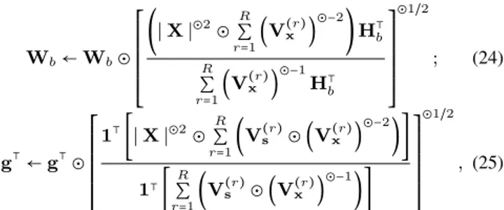
The multiplicative update rules for minimizing (19) using a majorize-minimize technique [30, 31] are given by (see [9] for derivation details): Hb← Hb⊙ ⎡⎢ ⎢⎢ ⎢⎢ ⎢⎢ ⎢⎣ W⊺b(∣ X ∣⊙2⊙ R ∑ r=1(V (r) x ) ⊙−2 ) Wb⊺ R ∑ r=1(V (r) x ) ⊙−1 ⎤⎥ ⎥⎥ ⎥⎥ ⎥⎥ ⎥⎦ ⊙1/2 ; (23) Wb← Wb⊙ ⎡⎢ ⎢⎢ ⎢⎢ ⎢⎢ ⎢⎣ (∣ X ∣⊙2⊙ R ∑ r=1(V (r) x ) ⊙−2 ) H⊺ b R ∑ r=1(V (r) x ) ⊙−1 H⊺b ⎤⎥ ⎥⎥ ⎥⎥ ⎥⎥ ⎥⎦ ⊙1/2 ; (24) g⊺← g⊺⊙ ⎡⎢ ⎢⎢ ⎢⎢ ⎢⎢ ⎢⎣ 1⊺[∣ X ∣⊙2⊙∑R r=1(V (r) s ⊙ (Vx(r)) ⊙−2 )] 1⊺[ R ∑ r=1(V (r) s ⊙ (V(r)x ) ⊙−1 )] ⎤⎥ ⎥⎥ ⎥⎥ ⎥⎥ ⎥⎦ ⊙1/2 , (25)
where⊙ denotes element-wise multiplication and exponentiation, matrix division is also element-wise, V(r)s , Vx(r) ∈ RF×N+ are the matrices of entries vs,f n(z(r)) and vx,f n(z(r)) respectively, X ∈
CF×Nis the matrix of entries xf nand 1 is an all-ones column
vec-tor of dimension F . Note that non-negativity of Hb, Wband g is
ensured provided that they are initialized with non-negative values.
A.3. Neural network architectures and training
The decoder and encoder network architectures are represented in Fig. 2 and Fig. 3 respectively. The "dense" (i.e. feed-forward fully-connected) output layers are of dimension L= 16 and F = 513 for the encoder and decoder, respectively. The dimension of all other layers was arbitrarily fixed to 128. RNN layers correspond to long short-term memory (LSTM) ones [40]. For the FFNN generative model, a batch is made of 128 time frames of clean speech power spectrogram. For the (B)RNN generative model, a batch is made 32 sequences of 50 time frames. Given an input sequence, all LSTM hidden states for the encoder and decoder networks are initialized to zero. For training, we use the Adam optimizer [35] with a step size of 10−3, exponential decay rates of 0.9 and 0.999 for the first and second moment estimates, respectively, and an epsilon of 10−8for preventing division by zero.
Dense (linear) Dense (tanh) (a) FFNN Dense (linear) RNN (b) RNN RNN RNN Dense (linear) Recurrent connection Feed-forward connection (c) BRNN
Fig. 2: Decoder network architectures corresponding to the speech generative models in Fig. 1.
RNN RNN RNN Dense (linear) Dense (linear) Sampling Dense (tanh) (a) BRNN RNN RNN Dense (linear) Dense (linear) Dense (tanh) Prediction Observation Update Recurrent connection Feed-forward connection Element-wise squared modulus Sampling (b) RNN Dense (linear) Dense (linear) Dense (tanh) Sampling (c) FFNN Fig. 3: Encoder network architectures associated with the decoder network architectures of Fig. 2.