HAL Id: hal-00551303
https://hal.archives-ouvertes.fr/hal-00551303v2
Submitted on 25 Jul 2011
HAL is a multi-disciplinary open access
archive for the deposit and dissemination of sci-entific research documents, whether they are pub-lished or not. The documents may come from teaching and research institutions in France or abroad, or from public or private research centers.
L’archive ouverte pluridisciplinaire HAL, est destinée au dépôt et à la diffusion de documents scientifiques de niveau recherche, publiés ou non, émanant des établissements d’enseignement et de recherche français ou étrangers, des laboratoires publics ou privés.
Spatio-temporal metamodeling for West African
monsoon
Anestis Antoniadis, Céline Helbert, Clémentine Prieur, Laurence Viry
To cite this version:
Anestis Antoniadis, Céline Helbert, Clémentine Prieur, Laurence Viry. Spatio-temporal metamodeling for West African monsoon. Environmetrics, Wiley, 2012, 23 (1), pp.24-36. �10.1002/env.1134�. �hal-00551303v2�
Spatio-temporal metamodeling for West African monsoon
Anestis Antoniadisa, Céline Helberta, Clémentine Prieura,∗, Laurence Virya
aUniversité de Grenoble, Laboratoire Jean Kuntzmann,
BP 53, 38041 Grenoble cedex, France
Abstract
In this paper, we propose a new approach for modeling and fitting high-dimensional res-ponse regression models in the setting of complex spatio-temporal dynamics. This study is motivated by investigating one of the major atmospheric phenomena which drives the rainfall regime in Western Africa : West African Monsoon. We are particularly interested in studying the influence of sea surface temperatures in the Gulf of Guinea on precipitation in Saharan and sub-Saharan.
Keywords: spatio-temporal modeling, filtering, multivariate penalized regression 1. Introduction
West African monsoon is the major atmospheric phenomenon which drives the rain-fall regime in Western Africa. It is characterized by a strong spatio-temporal variability whose causes have not yet been determined in an unequivocal manner. However, there is a considerable body of evidence suggesting that spatio-temporal changes in sea surface temperatures in the Gulf of Guinea and changes in the Saharan and sub-Saharan albedo are major factors. One of the interest of physicists is to perform sensitivity analysis on West African monsoon (see Messager et al. (2004)). The main tool for simulating preci-pitation is a regional atmospheric model (MAR) whose performances were evaluated by
∗. Corresponding author. Email : [email protected], phone : +33 (0)4 76 63 59 63, fax : +33 (0)4 76 63 12 63.
comparisons with precipitation data. Global sensitivity analysis of a model output consists in quantifying the respective importance of input factors over their entire range of values. Contrarily to deterministic approaches based on gradients, global analyses can be perfor-med on nonlinear systems. Many techniques have been developed in this field (see Saltelli et al. (2000) for a review). Performing a global sensitivity analysis implies running the model a large number of times. However it can not be realized by running the MAR, as we work on large discretization grids in space and time, thus dealing with huge dimen-sions. A way for overcoming this issue is to fit a stochastic model which approximates the MAR by taking into consideration the spatio-temporal dynamic of the underlying physi-cal phenomenon and with the ability to be run in a reasonable time. Statistiphysi-cal methods can be used to describe the behavior of a set of observations by focusing attention on the observations themselves rather than on the physical processes that produced them. One of those statistical methods is regression and in this paper we focus on the regression of precipitation on sea surface temperatures. As the numerical storage and processing of our model outputs (precipitation), as far as the statistical description of the data is concerned, require considerable computational resources, it will be run in a grid-computing environ-ment (see Caron et al. (2006)). This grid deployenviron-ment takes into account the scheduling of a huge number of computational requests and links with data-management between these requests, all of these as automatically as possible. It requires new developments which are not at the moment completely achieved. It explains why we fit our model with real data in this study : Reynolds climatological data on eighteen years (1983 to 2000) for sea surface temperatures and data collected by the french IRD (Institut de Recherche pour le Déve-loppement) during a period of eight years (1983 to 1990) for precipitation. The regression is achieved on the common period of observation (from 1983 to 1990). The poor quality of data over longer periods explain our restrictive choice (see Messager et al. (2004)). It
is clear that the study will be enhanced as soon as the grid deployment will be achieved, allowing a regression to be fitted on a longer period of eighteen years.
Functional data often arise from measurements on fine time grids, and many examples including environmental data can be found. In the following work, we consider on each sampled spatial point x (resp. y), as sample unit the year and the observed period is chosen from March to November, which corresponds to the active period of the monsoon phenomenon for our application. It is assumed that we have for each year an independent
realization of the stochastic process Xx (resp. Yy) that represents sea surface temperature
(resp. precipitation) along the reference period (March to November). This assumption of independence is certainly too strong to be realistic, as these data are collected sequentially over time and thus certainly present correlation among them. Prediction of such functio-nal time series has motivated the development of appropriate functiofunctio-nal models, the most popular being the autoregressive model of Bosq (2000) and its various extensions parti-cularly useful for prediction, see e.g. Besse (2000), Damon and Guillas (2002), Antoniadis and Sapatinas (2003) and Aguilera et al. (2008). However, how specifying a model is not clear for many functional time series. The Weighted Functional Principal Component Ap-proach (WFPCA) developed in Aguilera et al. (1999) is very interesting as it does not require any prespecified structure for the data. Applying a weighted scheme for estimating the sample mean and the covariance operator would probably be nonefficient in our case without further and stronger assumptions as we only have 8 observed segments (years). In the following, we have chosen FPCA as a dimensionality reduction technique based on the assumption that our observed segments are independent segments of the same continuous stochastic process (see Section 3). This choice was guided by recent results in Hörmann and Kokoszka (2010) which prove the robustness of this tool to weak dependence. More precisely Hörmann and Kokoszka investigate the performance of FPCA under what they
call m-approximation, which is a moment based notion of dependence for functional time series, not unreasonable on our data, even if the few number of years of observation does not allow us to validate this assumption. Finally, note that the four months gap (between two consecutive observation periods) makes this hypothesis even more plausible.
The present work introduces a new methodology for performing sensibility analysis of a heavy numerical model when handling spatio-temporal inputs and outputs. The metamodel construction process is based on several steps, including dimension reduction and regression. More precisely, the three major steps are the following : First, functional PCA of both the predictor (sea surface temperatures in the Gulf of Guinea) and the response (precipitations in Saharan and sub-Saharan) continuous-time processes is performed on the common period of observation for each location on the spatial grid. The Karhunen-Loève decomposition is then truncated because major part of variance is explained by only a few terms. This first step allows the reduction of the infinite dimension of temporal data to few coefficients. Secondly, a functional clustering algorithm is performed on the selected eigenfunctions to reduce the spatial dispersion of the Karhunen-Loève eigenfunctions (one decomposition per point). Few areas are identified where the decomposition (set of first eigenfunctions) can be considered constant for all the points of the area without losing accuracy. Thirdly, the relationship between inputs and outputs is modeled on the coefficients of the above decomposition through a double penalized regression approach. This methodology allows controlling the total number of predictors entering the model, and consequently facilitates the detection of important predictors. Finally, the precipitation curves obtained by our Þltering modeling are compared to observations themselves.
The paper is organized as follows. In Section 2 we give a brief description of the data. Our new approach for modeling both sea surface temperatures and precipitation is described in Section 3. Section 4 is devoted to the regression analysis. To conclude we mention in
Section 5 some of the many interesting perspectives of our study. 2. Data description
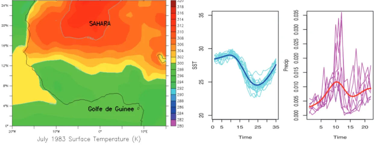
This section is devoted to the description of our data sets, chosen in accordance with physicists. The data used for sea surface temperatures (SST) are the so-called Reynolds climatological data, generated by an optimal interpolation technique (Reynolds and Smith (1994)) which uses satellite and in-situ data. We obtain a value for SST at each of the 516 points of a spatial grid G located in the Gulf of Guinea. West African Monsson is an almost periodic phenomenon, active from May to September. We work with a time discretization : we have weekly data from March to November (to cover the active period of the physical phenomenon). For these data we have eighteen years of observations, from 1983 to 2000.
Precipitation data have been recorded by the Institut de Recherche pour le
Dévelop-pement (IRD) on a spatial grid G" of size 382 located in Western Africa with the greatest
density of stations located between 5◦ N and 15◦ N (see Messager (2005)). We have daily
data whose mean is computed on 10 consecutive days from March to November, but only
from 1983 to 1990. After removing points on G" for which data were incomplete we work
with 368 points.
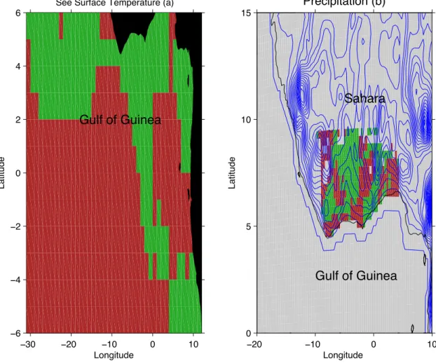
Below we present a map focusing on the region of interest around the Gulf of Guinea (see left panel of Figure 1). We also show on the right panel of the same figure the 18 time-dependent curves of sea surface temperatures and the 8 time-dependent curves of precipitation at some fixed spatial point.
[ Figure 1 about here. ]
Both inputs (SST) and outputs (precipitation) depend on space and time. Spatial and time discretizations result in very high-dimensional data which are difficult to analyze with
classical multivariate analysis. Functional data analysis (FDA) goes one big step further and seems the appropriate statistical tool to be used for analyzing our data for which time dynamics and spatial dynamics are a major component. Moreover an overarching theme in FDA is the necessity to achieve some form of dimension reduction of the infinite-dimensional data to finite and tractable dimensions and explains our choice to model inputs and outputs through spatio-temporal functional processes. For an introduction to the field of FDA, the two monographs by Ramsay and Silverman (2002, 2005) provide an accessible overview on foundations and applications, as well as a plethora of motivating examples. 3. Modeling inputs and outputs
The modeling for both inputs and outputs is described in this section. Our regression methodology to study the relationship between precipitation and the SST will be based on such modeling. Our method is a new filtering approach based on Karuhnen-Loève de-compositions and functional clustering. It allows reducing the dimensions involved in the data.
3.1. Functional modeling
Let T be a finite and closed interval of R. We usually refer to T as time. The spatial
regions of interest R and R" are both subsets of R2. In our applicative context, T is the
annual time period from March to November. The time period is the same for both SST and precipitation, even if time discretization differs. We model inputs (resp. outputs) on
the spatial grid G (resp. G") described in Section 2. The phenomenon under study is a
periodic phenomenon, with an active period from May to September, observed on N years (N is equal to 18 for SST and to 8 for precipitation). Let x be any point on the grid G. Following Yao et al. (2005b), we consider that the ith observed time-dependent trajectory at point x corresponds to a sampled longitudinal curve viewed as realizations of random
trajectories (Xx
i ), i = 1, . . . , , N, where Xix is assumed to belong to some Hilbert
functio-nal space H ⊂ L2(T ). These Xx
i’s are viewed as independent realizations of a stochastic
process Xx with unknown smooth mean function EXx(t) = µ
Xx(t), and covariance
func-tion Cov (Xx(s), Xx(t)) = G
Xx(s, t). The assumption of independence is discussed in the
introduction (see Section 1).
It is well known that under very mild conditions, there exists an orthogonal expansion
of GXx (in the L2 sense) in terms of eigenfunctions em(x,·) with associated eigenvalues
ρm(x) (arranged in nonincreasing order), that is,
GXx(s, t) =
!
m≥1
ρm(x)em(x, s)em(x, t), s, t∈ T .
The random function Xx(t)where t denotes time and x location, may be decomposed into
an orthogonal expansion Xx(t) = µ Xx(t) + ∞ ! m=1 αm(x)em(x, t), t∈ T .
The above representation of a random function is known as the Karhunen-Loève expansion, although in the meteorological literature it is known as the Empirical Orthogonal Function
(EOF) expansion. It can be shown that the truncated decomposition with Nx terms (that
is keeping at location x the first Nx principal components)
Xtrunc,x(t) = µXx(t) + Nx
!
m=1
αm(x)em(x, t), t∈ T . (1)
minimises the mean integrated squared error E"#T[Xx(t)− Xtrunc,x(t)]2dt$. The spectral
representation is optimal in the sense that this error is minimum compared to Nx terms of
any orthogonal system (see, e.g. Cohen and Jones (1977)). In our case we take Nx as the
truncation needed at point x to explain more than 80 % of the variance.
In our analysis, for each spatial grid point in the Gulf of Guinea and each year of observation, sea surface temperature is measured during the active period on a temporal
grid. A Karhunen-Loève decomposition is then performed at each location on the spatial grid (see e.g. Yao et al. (2005b)). In order to achieve an optimal (in the least-squares sense)
representation of the observed process, the appropriate number of terms Nx depends on
the location on the spatial grid. To simplify the analysis we will consider in the following
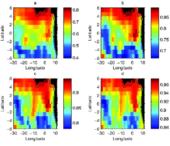
that Nx is bounded above by a number M independent of x. As one can see from Figure
2 such an assumption with M = 2 (i.e. with a cumulative percentage of variance explained that is larger than 70%) seems perfectly valid for our data on sea surface temperatures.
[ Figure 2 about here. ]
In our application, the number and shape of the eigenfunctions patterns over time are not known and the lack of stationarity over space makes them dependent on the spatial lo-cation. The estimation of these eigenfunctions at different spatial locations generates great amounts of high-dimensional data. It seems therefore reasonable to assume some kind of local stationarity by assuming that at least the resulting eigenfunctions are spatially pie-cewise constant. Clustering algorithms become then crucial in reducing the dimensionality of such data. The choice of the clustering approach is described in Section 3.3. For the
moment let us just assume that we know that there exist L1 points x0,1, . . . , x0,L1 (with
L1 ∈ N∗) on the spatial grid G partitioning G = ∪L1l=1Gl into L1 subregions Gl that appear
as a “natural” system of spatial coordinates that reflects the underlying internal and lo-cal stationary structures of the data. Given such a partition, for any x on G, there exist
l ∈ {1, . . . , L1} and a specific point x0,l in Gl such that we can approximate Xx(t) by
% Xx(t) = µXx(t) + M ! m=1 % αm(x)em(x0,l, t), t∈ T , (2) with %αm(x) = # T X%x(t)em(x0,l, t)dt, for m = 1, . . . , M.
The modeling for precipitation follows the same lines, leading to L2 fixed grid points
y0,1, . . . , y0,L2 (with L2 ∈ N∗) on the spatial grid G" partitioning G" = ∪L2l=1Gl" into L2
subregions G"
l. Then, given such a partition, for any y on G" there exist l ∈ {1, . . . , L2} and
a specific point y0,l in Gl" such that we can approximate Yy(t) by
% Yy(t) = µYy(t) + K ! k=1 % βk(y)fk(y0,l, t), t∈ T , (3) with %βk(y) = # T Y% y(t)f
k(y0,l, t)dt for k = 1, . . . , K. The truncation number K is also
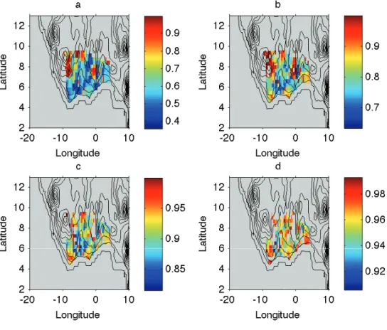
assumed not to depend on y ∈ G" and will be chosen equal to 2 for our test case (see Figure
3).
[ Figure 3 about here. ]
In the following, if nSST (resp. nP) denotes the number of points on G (resp. G"), we
define the nSST-dimensional (resp. the nP-dimensional) vectors
αm = (α%m(x1), . . . ,α%m(xnSST))t, m = 1, . . . , M
and
βk =&β%k(y1), . . . , %βk(ynP)
't
, k = 1, . . . , K.
Note that in our application nSST = 516 and nP = 368.
3.2. Estimation procedure
We now describe our estimation procedure, following the main lines in Yao et al. (2005a). The methodology described below and used for our analysis has been implemented in Matlab and is freely available in the PACE (principal analysis by conditional expectation) package, downloadable from the internet (see Yao et al. (2010)).
We only deal here with SST since the procedure is the same for precipitation. Let x be
any point on the spatial grid G. Assume x ∈ Gl for some l ∈ {1, . . . , L1}. In a first step,
and eigenfunctions are assumed to be smooth and we therefore use local linear smoothers (Fan and Gijbels, (1996)) for function and surface estimation, fitting local lines in one dimension and local planes in two dimensions by weighted least squares. The bandwidth b necessary for local smoothing is chosen by minimizing the cross-validation score given by
CV (b) = (Ni=1(Tj=1{Xx
i(tj)− )µ(−i)(tj; b)}2/N, where t1, . . . , tT is the time discretization
of T , N is the number of observed curves at x and )µ(−i)(t
j; b) is the estimation of µXx(tj)
obtained without using the ith curve. To estimate the cross-covariance surface GX(s, t),
s, t ∈ T we have used two-dimensional scatterplot smoothing. The raw cross-covariances
GX,i(tj, tk) = (Xix(tj)− )µXx(tj)) (Xix(tk)− )µXx(tk)) are considered as input for the
two-dimensional smoothing step. More precisely, the local linear surface smoother for the
cross-covariance surface GX(s, t) is obtained as in Yao et al. (2005a)by minimizing :
N ! i=1 ! 1≤j,k≤T K2 * tj− s h1 ,tk− t h2 + {GX,i(tj, tk)− f(β, (s, t), (tj, tk))}2
with respect to β = (β0, β1,1, β1,2), leading to )GX(s, t) = )β0(s, t), where f(β, (s, t), (tj, tk)) =
β0+β1,1(s−tj)+β1,2(t−tk), K2is a given two-dimensional kernel, and where the bandwidths
h1 and h2 are chosen again by cross-validation.
The estimates of eigenfunctions and eigenvalues correspond to the solutions )em(x0,l,·)
and )ρm of the following integral equations :
,
T
)
GX(s, t))em(x0,l, s)ds =ρ)m)em(x0,l, t),
where the )em(x0,l,·) are subject to
#
T )em(x0,l, t)2dt = 1and
#
T )ek(x0,l, t))em(x0,l, t)dt = 0for
m &= k ≤ M. The eigenfunctions are estimated by discretizing the smoothed covariance, as
described e.g. in Rice and Silverman (1991) or Capra and Müller (1997).
Finally, to complete the estimation procedure for SST, we have to estimate %αi
m(x), for
i = 1, . . . , N and m = 1, . . . , M. We use the following projection estimates :
T
!
j=2
Xix(tj))em(x0,l, tj)(tj− tj−1),
which are just numerical integration versions of %αi
m(x) =
#
T Xix(t))em(x0,l, t)dt, for m =
1, . . . , M. The estimation for each individual curve is needed in Section 4 for the selection
procedure of the regression. 3.3. Functional clustering results
As mentioned previously, clustering algorithms are crucial in reducing the dimensiona-lity of our data. The number and shape of the eigenfunctions patterns over time are not known. An ideal clustering method would provide a statistically significant set of clusters (and therefore of spatial regions) and curves derived from the data themselves without re-lying on a pre-specified number of clusters or set of known functional forms. Further, such a method should take into account the between time-point correlation inherent in time series data. Some popular methods such as k-means clustering (see Hartigan and Wong (1978)), self-organizing maps (SOM) (see Kohonen (1997)) or hierarchical clustering (see Eisen et al. (1998)) do not satisfy this pre-requisite. One promising approach is to use a general multivariate Gaussian model to account for the correlation structure ; however, such a model ignores the time order of the eigenfunctions. The time factor is important in interpreting the clustering results of time series data. A curve-based clustering method called FCM was introduced in James and Sugar (2003) to cluster sparsely sampled time course genomic data. Similar approaches were proposed in Luan and Li (2003) to analyze time course gene expression data. In these methods, the mean gene expression profiles are modeled as linear combinations of spline bases. However, with different choices of bases or of the number of knots, one could get an array of quite different estimates of the underlying curves. Effective methods or guidance on how to select the basis or the number of knots
are still lacking, which hinders the effective use of these methods in real applications. Here, we have used a data-driven clustering method, called smoothing spline clustering (SSC), that overcomes the aforementioned obstacles using a mixed-effect smoothing spline model and a rejection-controlled EM algorithm (see Ma et al. (2006)). A distinguishing feature of SSC is that it accurately estimates individual eigenvalue profiles and the mean eigen-function profile within clusters simultaneously, making it extremely powerful for clustering time series data. Let us now present the way we fixed the number of clusters for our test case.
Sea surface temperatures :
We first performed the SSC approach on the 516 estimated first eigenfunctions t → )e1(x,·)
obtained by the Karuhnen-Loève decomposition at each point x of the spatial grid G. To determine a convenient number K of clusters several data- driven strategies can be defined. For this study we use an information theoretic point of view provided by Sugar
and James (2003), based on the transformed distortion curve (K, dK), where dK denotes
the minimum achievable distortion associated with fitting K centers to the data. Sugar and James’ criterion applied to our data leads to K = 3. Given the lack of observations, interpretation of the map with three clusters appeared difficult for physicists. We thus prefer hereafter a choice of two clusters, which seems to be more robust. Projection on the map for two clusters is drawn on the left panel (a) of Figure 5. A relevant factor for discrimination validated by physicists is the distance to the coast.
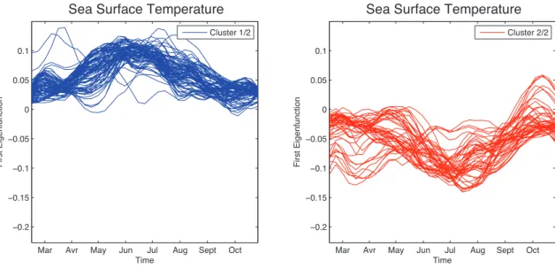
The objective of Figure 4 is to see the overall trend of the first eigenfunctions over time, uncovering spatial-specific variation patterns. More specifically, we collect for each cluster
the estimated curves t → )e1(x,·), x ∈ G. It shows that the temperature differences from
one year to another are maximum around June-July for the first group, and July-August for the second one.
[ Figure 4 about here. ]
Let us now consider what happens for the second eigenfunctions t → e2(x,·), x ∈ G.
Classifying the estimated curves t → )e2(x,·) on each of the two clusters obtained by
applying the SSC procedure on the 18 curves t → )e1(x,·) showed that the clustering
structure seems also adapted for discriminating the second eigenfunctions. It thus validates Decomposition (2) with M = 2 announced in Subsection 3.1. It remains to choose the
representative points x0,1 and x0,2 for each cluster. We considered the centroid for each
cluster. These two points were not necessarily on the grid G, thus for each cluster we chose the point on the grid which is the closest to the centroid.
Precipitation :
The procedure adopted for analyzing precipitation is similar. Sugar and James’ criterion leads to three clusters reduced to K = 2 clusters for sake of robustness. Projection on the map for two clusters is drawn on the right panel (b) of Figure 5. From physicists point of view, a plausible relevant factor for discrimination is the topography.
[ Figure 5 about here. ]
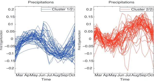
Considering two spatial clusters, in Figure 6 we collect for each cluster the estimated
curves t → )f1(y, t), y ∈ G". It shows a significant dipersion late August early September,
when the phenomenon of rain vanishes.
[ Figure 6 about here. ]
Investigating what happens on the second eigenfunctions t → f2(y,·), y ∈ G", we can
conclude that no further clustering structure appears in the estimated curves which
sup-ports the fact that using the two clusters (denoted by G"
the first eigenfunctions for discriminating the clusters makes sense. It thus validates again Decomposition (3) with K = 2 announced in Subsection 3.1. The difference is that,
contra-rily to what happens for SST, we do not define t → f2(y0,l, t) as the second eigenfunction
obtained at point y0,l but as the mean curve t → f2(t) of all curves t → f2(y, t), y ∈ G".
Thus it does not depend on space. It remains to choose the representative points y0,1 and
y0,2 for each cluster. We considered the centroid for each cluster. These two points are not
necessarily on the grid G", thus for each cluster we chose the point on the grid that is the
closest to the corresponding centroid.
Hence for both precipitation and sea surface temperatures, we obtain a decomposition where the basis functions are functions depending on time only and whose coefficients
are spatially indexed and time independent. The relative mean squared error (MSErel)
for the reconstruction of sea surface temperatures and precipitation is estimated by
leave-one-out cross-validation (see eq. (4) below for the definition of MSErel). The panels in
Figure 7 below display this relative mean squared error for SST reconstruction (left) and precipitation (right) on the appropriate map.
Leave-one-out cross-validation relative mean squared error estimation for SST at each point x ∈ G is defined by MSErel,SST(x) = 1 22 T ! j=1 1 18 (18 k=1 & % X(−k),x(t j)− Xkx(tj) '2 1 18 (18 k=1(Xkx(tj))2 , (4)
where %X(−k),x(tj) is the estimation of Xx(tj) obtained without using the kth curve Xkx(·).
The procedure for the estimation of the relative mean squared error for precipitation is similar.
[ Figure 7 about here. ]
4. Multivariate regression model, a double penalized approach
This section concerns the regression approach we have adopted for modeling the rela-tion between inputs and outputs (see Subsecrela-tion 4.1). We also discuss in this Secrela-tion the selection procedure of the tuning parameters for our application (see Subsection 4.2). 4.1. Regression procedure
As mentioned in the introduction, we intend to use a novel method recently developed by Peng et al. (2010) in integrated genomic studies which we describe below for the sake of
completeness. The method uses an $1-norm penalty on a least squares procedure to control
the overall sparsity of the coefficient matrix in a multivariate linear regression model. In addition, it also imposes a group sparse penalty, which in essence is the same as the group lasso penalty proposed by Bakin (1999), Antoniadis and Fan (2001) and Obozinski et al.
(2008). This penalty puts a constraint on the $2 norm of regression coefficients for each
predictor, which thus controls the total number of predictors entering the model, and consequently facilitates the detection of important predictors.
More precisely, consider a multivariate regression problem with q response variables
Y1, . . . , Yq and p prediction variables X1, . . . , Xp :
Yj =
p
!
i=1
XiBij + %j, j = 1, . . . , q, (5)
where the error terms %1, . . . , %q have a joint distribution with mean 0 and covariance Σ. In
the above, we assume without any loss of generality that all the response and prediction variables are standardized to have zero mean and thus there is no intercept term in equation (5). Our primary goal is to identify non-zero entries in the p×q regression coefficient matrix
B = (Bij) based on n i.i.d. samples from the above model which is exactly the problem
proportional to the conditional correlation Cor(Yj, Xi|X−(i)), where X−(i) :={Xi" : 1≤ i" &=
i ≤ p}. In the following, we use Yj = (Yj1, Yj2, . . . , Yjn)T and Xi = (Xi1, Xi2. . . , Xin)T to
denote respectively the sample of the jth response variable and that of the ith prediction
variable. We also use Y = (Y1 : · · · : Yq) to denote the n × q response matrix, and use
X = (X1 :· · · : Xp)for the n ×p prediction matrix. We shall focus on the cases where both
qand p are larger than the sample size n. For example, in the applied study of West African
Monsoon discussed later, we regress -α1, α2
.
on&β1, β2'. Hence, for this application, the
sample size is 8, while the number of spatial components are respectively p = 2 × nSST and
q = 2× nP. In the application nSST = 516 and nP = 368. When q > n, whatever the value
of p is, the ordinary least square (OLS) solution is not unique, and regularization becomes indispensable. The choice of suitable regularization depends heavily on the type of data
structure we envision. Recently, $1-norm based sparsity constraints such as lasso (Tibshirani
(1996)) have been widely used under such high-dimension-low-sample-size settings. In our
application, we will impose an $1-norm penalty on the coefficient matrix B to control the
overall sparsity of the multivariate regression model but in addition, we put constraints on the total number of predictors entering the model which is essentially the remMap idea. This is achieved by treating the coefficients corresponding to the same predictor (one row
of B in model (5) as a group, and then penalizing their $2 norm. A predictor will not be
selected into the model if the corresponding $2-norm is shrunken to 0. Thus this penalty
facilitates the identification of master predictors which affect (relatively) many response variables. Specifically, for model (5), we wiil use the following criterion
$(λ,µ)(Y, B) = 1 2*Y − XB* 2 F + λ p ! j=1 *Cj · Bj*1+ µ p ! j=1 *Cj · Bj*2, (6)
where C is a p × q 0-1 matrix indicating the coefficients of B on which penalization is
imposed. In the above equation Cj and Bj are the jth rows of C and B respectively, while
* ·*F denotes the Frobenius norm of matrices, * · *1 and * ·*2 are respectively the $1 and
$2 norms of vectors and “·” stands for the Hadamard product (entry-wise multiplication).
The selection matrix C is pre-specified based on prior knowledge : if we know in advance
that predictor Xi affects response Yj , then the corresponding regression coefficient Bij will
not be penalized and we set Cij = 0. When there is no such prior information, C can be
simply set to a constant matrix Cij = 1. Finally, an estimate of the coefficient matrix B is
)
Bλ,µ:=argminB$(λ,µ)(Y, B).
In the above criterion function, the $1 penalty induces the overall sparsity of the
co-efficient matrix B. The $2 penalty on the row vectors Cj · Bj induces row sparsity of the
product matrix C·B. As a result, some rows are shrunken to be entirely zero. Consequently, predictors which affect relatively more response variables are more likely to be selected into
the model. We will refer to the proposed estimator )Bλ,µas the remMap (REgularized
Mul-tivariate regression for identifying MAster Predictors) estimator in connexion with the remMap theory and R-package developed by Peng et al. (2010) for regularized multiva-riate Regression for identifying master predictors in integrative genomics studies of breast cancer.
4.2. Implementation and results
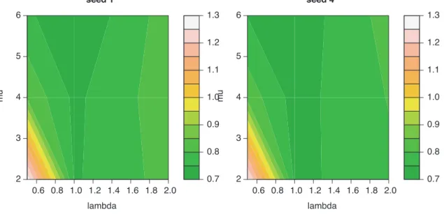
In this subsection, we describe the different steps for the implementation of the rem-MAP procedure on our application. A first step is to fit both parameters λ and µ. These parameters are adjusted by v-fold cross-validation. The prediction error obtained by 4-fold cross-validation is drawn on Figure 8 below. We note that there does not exist a unique minimum. For λ = 1 and µ = 4, the error seems to reach a value close to the minimum.
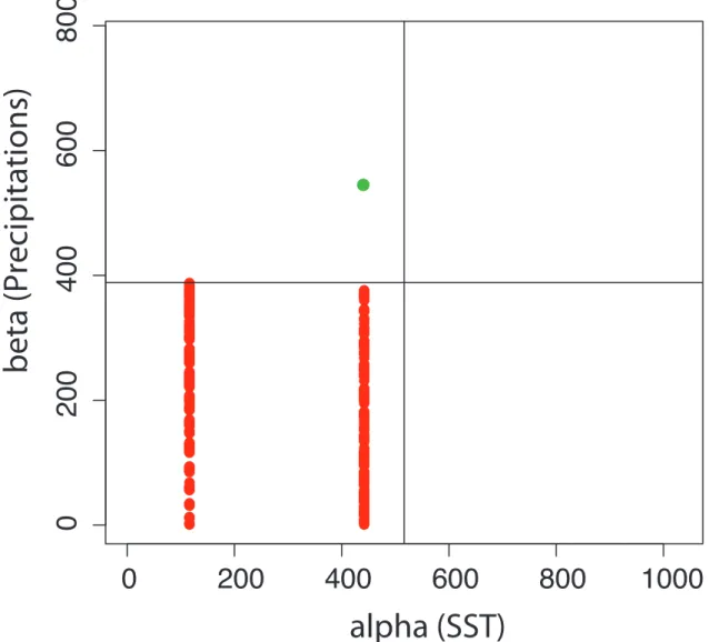
On Figure 9 we note that the regression coefficients matrix B, estimated using λ = 1 and
µ = 4for the penalties, is sparse. This is a consequence of using the remMAP methodology.
[ Figure 9 about here. ]
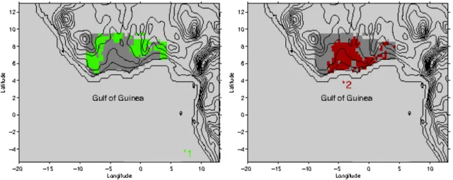
It seems quite interesting to display on a map the spatial points on the grid G
corres-ponding to the nonzero rows of the matrix B (left) and the spatial points on G" influenced
by the nonzero rows of B (right) (see Figure 10 below). As one may see, the two regions seem complementary and cover quite well the region of interest for precipitation.
[Figure 10 about here. ]
Using the results of the regression and given the retained regression coefficients we the
proceed to the reconstruction of Precipitation on the grid G". Define first
&
β1,reg, β2,reg'T =-α1, α2. )B .
Then for l = 1, 2, for y ∈ G"
l, let
Yy,reg(t) =)µYy(t) + β1,regf)1(y0,l, t) + β1,regf)2(t) .
The relative mean squared error (RMSE) estimated by leave-one-out cross-validation (see (7) below) is displayed on the map (see Figure 11). Notice however some points of high RMSE which are close to the coast. We have also plot the annual and weekly boxplots for the relative MSE (see Figure 12). The relative error is between 0.3 and 0.4 which is not so bad if we consider we did not have many observations to conduct the study. As one can see on the right panel of the figure this error is not constant over time, with bad reconstructions for some weeks.
MSEP recip,reg(y) = 1 22 22 ! j=1 1 8 (8 k=1 * Y(−k),y,reg(tj)− /Y%ky(tj) +2 1 8 (8 k=1 * 0 % Yky(tj) +2 , (7)
with 0Y%ky(tj) =µ)Yy(tj) + 0β%1k(y) )f1(y0,l, tj) + 0β%2k(y) )f2(tj).
[Figure 11 about here. ]
[Figure 12 about here. ]
Finally, on Figure 13 below we plotted for some fixed points in G" the curve
recons-tructed by regression (continuous line) for precipitation, the one obtained by the filtering modeling of Section 3 (circles) and the observations themselves (dots). As one can see the regression prediction curve somehow smooths the observations in quite a natural way and the methodology seems promising for pursuing via this model a sensitivity analysis, but this is beyond the scope of the present work.
[Figure 13 about here. ]
5. Conclusion and perspectives
Motivated in investigating the West African Monsoon, we present a new approach for modeling and fitting high-dimensional response regression models in the setting of complex spatio-temporal dynamics. We were particularly interested in developing an appropriate regression based methodology for studying the influence of sea surface temperatures in the Gulf of Guinea on precipitation in Saharan and sub-Saharan. However, one central issue in the analysis of such data consists in taking into account the spatio-temporal dependence
of the observations. For most of the applications that we are aware of the spatio-temporal dynamics are usually modeled as time function-valued (spatially stationary) processes al-lowing the development of efficient prediction procedures based on appropriate principal component like decompositions and regression. In practice, however, many observed spatial functional time series cannot be modeled accurately as stationary. To handle spatial varia-tion in a natural way we have segmented the space into regions of similar spatial behavior using in the process an efficient clustering technique that clusters the times series into groups that may be considered as stationary so that in each group more or less standard regression prediction procedures can be applied. Furthermore to avoid regression models that are far too complex for prediction, and inspired by similar approaches used in modern genomic data analysis we have used an appropriate regularization method that has proven to be quite efficient for the data we have analyzed. However, a major lack in this study is that it was implemented with only 8 years of observations. To overcome this issue, the authors have in mind to perturb initial maps of SST and then to run the regional atmos-pheric model MAR on these new inputs. Such a simulation study involves the development of MAR on a computer-grid environment to be achieved. Recall that fitting an appropriate metamodel is a necessary preliminary step to sensitivity analysis in our context where the code requires considerable computational resources. This simulation study will be perfor-med, as far as the sensitivity analysis, in a future work. The main goal achieved in the present work is to present an original and innovative methodology to reduce the dimension as a first step towards sensitivity analysis.
Acknowledgments
The authors are grateful to two referees and to an Associate Editor for their helpful comments and suggestions. They also thank Peter Guttorp, Editor-in-Chief for the journal
Environmetrics, as far as Wenceslao Gonzalez-Manteiga for the initiative of this special issue.
This work has been partially supported by French National Research Agency (ANR)
through COSINUS program (project COSTA-BRAVA n◦ ANR-09-COSI-015) and the IAP
Research Network P6/03 of the Belgian State (Belgian Science Policy). References
[1] Aguilera, A., Ocana, F., and Valderrama, M. (1999). Forecasting time series by func-tional PCA. Discussion of several weighted approaches. Computafunc-tional Statistics, 14(3), 443.
[2] Aguilera, A., Escabias, M., and Valderrama, M. (2008). Forecasting binary longitudinal data by a functional PC-ARIMA model. Computational Statistics & Data Analysis, 52(6), 3187–3197.
[3] Antoniadis, A. and Fan, J. (2001). Regularization of wavelets approximations (with discussion). J. Amer. Statist. Assoc., 96(455), 939–963.
[4] Antoniadis, A. and Sapatinas, T. (2003). Wavelet methods for continuous-time pre-diction using Hilbert-valued autoregressive processes. Journal of Multivariate Analysis, 87(1), 133–158.
[5] Bakin, S. (1999). Adaptive regression and model selection in data mining probems. Ph.D. thesis, Australian National University, Cambera, Australia.
[6] Besse, P. C. (2000). Autoregressive forecasting of some functional climatic variations. Scandinavian Journal of Statistics, 27(4), 673–687.
[7] Bosq, D. (2000). Linear processes in function spaces, volume 149 of Lecture Notes in Statistics. Springer-Verlag, New York. Theory and applications.
[8] Capra, W. B. and Müller, H. G. (1997). An accelerated-time model for response curves. Journal of the American Statistical Association, (92), 72–83.
[9] Caron, E., Chouhan, P. K., and Dail, H. (2006). Godiet : A deployment tool for dis-tributed middleware on grid’5000. In EXPGRID workshop. Experimental Grid Testbeds for the Assessment of Large-Scale Distributed Apllications and Tools., Paris. France. HPDC-15, IEEE.
[10] Cohen, A. M. and Jones, D. E. (1977). A technique for the solution of eigenvalue problems. J. Inst. Math. Appl., 20(1), 1–7.
[11] Damon, J. and Guillas, S. (2002). The inclusion of exogenous variables in functional autoregressive ozone forecasting. Environmetrics, 13(7), 759–774.
[12] Eisen, M. B., Spellman, P. T., Brown, P. O., and Botstein, D. (1998). Cluster analysis and display of genome-wide expression patterns. Proc. Natl. Acad. Sci. USA, 95, 14863– 14868.
[13] Fan, J. and Gijbels, I. (1996). Local Polynomial Modelling and Its Application. Chap-man and Hall, London.
[14] Hartigan, J. A. and Wong, M. A. (1978). A k-means clustering algorithm. App. Statist., 28, 100–108.
[15] Hörmann, S. and Kokoszka, P. (2010). Weakly dependent functional data. The Annals of Statistics, 38(3), 1845–1884.
[16] James, G. and Sugar, C. (2003). Clustering for sparsely sampled functional data. Journal of the American Statistical Association, 98, 397–408.
[17] Kohonen, T. (1997). Self-Organizing Maps. Springer, New York.
[18] Luan, Y. and Li, H. (2003). Clustering of time-course gene expression data using a mixed-effects model with b-spline. Bioinformatics, 19, 474–482.
[19] Ma, P., Castillo-Davis, C. I., Zhong, W., and Liu, J. S. (2006). A data-driven clustering method for time course gene expression data. Nucleic Acids Research, 34(4), 1261–1269. [20] Messager, C. (2005). Couplage des composantes continentale et atmosphérique du cycle de l’eau aux échelles régionale et climatique. Application à l’Afrique de l’Ouest. Ph.D. thesis, University Joseph Fourier, Grenoble, France.
[21] Messager, C., Gallée, H., and Brasseur, O. (2004). Precipitation sensitivity to regional sst in a regional climate simulation during the west african monsoon for two dry years. Climate Dynamics, 22, 249–266.
[22] Obozinski, G., Wainwright, M. J., and Jordan, M. I. (2008). Union support recovery in high-dimensional multivariate regression. Technical Report (to appear in Annals of Statistics) 761, Dept. of Statistics. University of California at Berkeley.
[23] Peng, J., Zhu, J., Bergamaschi, A., Han, W., Noh, D.-Y., Pollack, J. R., and Wang, P. (2010). Regularized multivariate regression for identifying master predictors with application to integrative genomics study of breast cancer. Annals of Applied Statistics, 4(1), 53–77.
[24] Ramsay, J. O. and Silverman, B. W. (2002). Applied Functional Data Analysis : Methods and Case Studies. Springer-Verlag.
[25] Ramsay, J. O. and Silverman, B. W. (2005). Functional data analysis. Springer-Verlag, second edition edition.
[26] Reynolds, R. W. and Smith, M. T. (1994). Improved global sea surface temperature analysis using optimal interpolation. Journal of Climate, 7, 929–948.
[27] Rice, J. A. and Silverman, B. W. (1991). Estimating the mean and covariance structure nonparametrically when the data are curves. J. Roy. Statist. Soc. Ser. B, 53(1), 233–243. [28] Saltelli, A., Chan, K. P. S., and Scott, E. M. (2000). Sensitivity Analysis. John Wiley
& Sons, New York.
[29] Sugar, C. A. and James, G. M. (2003). Finding the number of clusters in a dataset : an information-theoretic approach. Journal of the American Statistical Association, 98(463), 750–763.
[30] Tibshirani, R. (1996). Regression shrinkage and selection via the lasso. J. Roy. Statist. Soc. Ser. B, 58, 267–288.
[31] Yao, F., Müller, H.-G., and Wang, J.-L. (2005a). Functional data analysis for sparse longitudinal data. J. Amer. Statist. Assoc., 100(470), 577–590.
[32] Yao, F., Müller, H.-G., and Wang, J.-L. (2005b). Functional linear regression analysis for longitudinal data. Ann. Statist., 33(6), 2873–2903.
[33] Yao, F., Liu, B., Müller, H.-G., and Wang, J.-L. (2010). PACE 2.7 . University of California at Davis, http ://anson.ucdavis.edu/-mueller/data/programs.html.
Figures
Table des figures
1 Left : Zone of interest for the study of West-African monsoon ; Right :
Time-dependent curves for SST (left) resp. Precip (right) for each of the 18 (resp.
8) years of observations for some fixed spatial point x ∈ G (resp. x" ∈ G"). 27
2 Percent cumulative variance for the SST on the map explained by
recons-tructing the SST using (a) one term (b) two terms (c) three terms and (d)
four terms in the corresponding truncated Karhunen-Loève expansion . . . 28
3 Percent cumulative variance for precipitation on the map explained by
re-constructing the precipitation process using (a) one term (b) two terms (c) three terms and (d) four terms in the corresponding truncated
Karhunen-Loève expansion. . . 29
4 Estimated curves for the first eigenfunction by cluster . . . 30
5 Projection of (a) SST, (b) precipitation, on the map for two clusters . . . . 31
6 Precipitation data : estimated curves by cluster for the first eigenfunction. 32
7 (Relative Mean Squared Error for the reconstruction of SST (left) and of
Precipitation (right) . . . 32
8 Cross validation for the choice of λ and µ (with two different germs) . . . . 33
9 Regression coefficients matrix B estimated with λ = 1 and µ = 4 . . . 34
10 Spatial location for the average responses indicated by the retained
coeffi-cients for both predictors (points 1 and 2 on the map). . . 35
11 Relative MSE for the reconstructed precipitation by regression on the map. 36
13 For 4 spatial points selected in the domain G" a display of the reconstructed
precipitation curve (red), the reconstruction curve with truncated
Karhunen-Loève decomposition (circles) and the observed precipitation (dots). . . . 38
0 5 15 25 35 20 25 30 35 Time SST 5 10 15 20 0.000 0.005 0.010 0.015 0.020 0.025 0.030 0.035 Time Precip
Figure 1: Left : Zone of interest for the study of West-African monsoon ; Right : Time-dependent curves for SST (left) resp. Precip (right) for each of the 18 (resp. 8) years of observations for some fixed spatial point x ∈ G (resp. x!∈ G!).
Figure 2: Percent cumulative variance for the SST on the map explained by reconstructing the SST using (a) one term (b) two terms (c) three terms and (d) four terms in the corresponding truncated Karhunen-Loève expansion
Figure 3: Percent cumulative variance for precipitation on the map explained by reconstructing the preci-pitation process using (a) one term (b) two terms (c) three terms and (d) four terms in the corresponding truncated Karhunen-Loève expansion.
Mar Avr May Jun Jul Aug Sept Oct −0.2 −0.15 −0.1 −0.05 0 0.05 0.1 Time First Eigenfunction
Sea Surface Temperature
Mar Avr May Jun Jul Aug Sept Oct
−0.2 −0.15 −0.1 −0.05 0 0.05 0.1 Time First Eigenfunction
Sea Surface Temperature
Cluster 2/2 Cluster 1/2
Figure 4: Estimated curves for the first eigenfunction by cluster
−30 −20 −10 0 10 −6 −4 −2 0 2 4 6 Latitude Longitude
See Surface Temperature (a)
Gulf of Guinea −20 −10 0 10 0 5 10 15 Precipitation (b) Longitude Latitude Sahara Gulf of Guinea
Time −0.2 −0.15 −0.1 −0.05 0 0.05 0.1 0.15 0.2 First Eigenfunction
Mar ApMay Jun Jul AugSep Oct Time
Cluster 1/2 Cluster 2/2
Mar ApMay Jun Jul AugSep Oct −0.2 −0.15 −0.1 −0.05 0 0.05 0.1 0.15 0.2 First Eigenfunction Precipitations Precipitations
Figure 6: Precipitation data : estimated curves by cluster for the first eigenfunction.
Figure 7: (Relative Mean Squared Error for the reconstruction of SST (left) and of Precipitation (right)
0.7 0.8 0.9 1.0 1.1 1.2 1.3 0.6 0.8 1.0 1.2 1.4 1.6 1.8 2.0 2 3 4 5 6 seed 1 lambda mu 0.7 0.8 0.9 1.0 1.1 1.2 1.3 0.6 0.8 1.0 1.2 1.4 1.6 1.8 2.0 2 3 4 5 6 seed 4 lambda mu
0
200
400
600
800
1000
0
200
400
600
800
alpha (SST)
beta (Precipitations)
Figure 9: Regression coefficients matrix B estimated with λ = 1 and µ = 4
Figure 10: Spatial location for the average responses indicated by the retained coefficients for both pre-dictors (points 1 and 2 on the map).
Figure 11: Relative MSE for the reconstructed precipitation by regression on the map.
0.0
0.5
1.0
1.5
2.0
RMSE
1 5 9 13 180
2
4
6
8
10
TimeRMSE
5 10 15 20 0.000 0.005 0.010 0.015 Time Precipitations regression filtering observ. 5 10 15 20 0.000 0.005 0.010 0.015 Time Precipitations Time Time 5 10 15 20 0.000 0.005 0.010 0.015 Precipitations 5 10 15 20 0.000 0.005 0.010 0.015 Precipitations
Figure 13: For 4 spatial points selected in the domain G!a display of the reconstructed precipitation curve
(red), the reconstruction curve with truncated Karhunen-Loève decomposition (circles) and the observed precipitation (dots).