HAL Id: hal-02512793
https://hal.archives-ouvertes.fr/hal-02512793
Submitted on 19 Mar 2020
HAL is a multi-disciplinary open access
archive for the deposit and dissemination of
sci-entific research documents, whether they are
pub-lished or not. The documents may come from
teaching and research institutions in France or
abroad, or from public or private research centers.
L’archive ouverte pluridisciplinaire HAL, est
destinée au dépôt et à la diffusion de documents
scientifiques de niveau recherche, publiés ou non,
émanant des établissements d’enseignement et de
recherche français ou étrangers, des laboratoires
publics ou privés.
Input signal and model structure analysis for the HVDC
link POD control
Mohamed Belhocine, Bogdan Marinescu, Florent Xavier
To cite this version:
Mohamed Belhocine, Bogdan Marinescu, Florent Xavier. Input signal and model structure analysis
for the HVDC link POD control. PowerTech, Jun 2017, Manchester, France. �hal-02512793�
Input signal and model structure analysis for the
HVDC link POD control
M. Belhocine
Ecole Centrale Nantes-IRCCyN Nantes, France
B. Marinescu
Ecole Centrale Nantes-IRCCyN Nantes, France
F. Xavier
RTE R&D Division Versailles, France [email protected]
Abstract—In this paper, the input signals and the control model structure of the HVDC link POD control are studied. First, a benchmark is proposed to investigate the input signal selection of the POD controller. Next, by considering different situations, it is shown, based on the residues criteria, that the choice of the input signal depends on the parameters of the system. More precisely, the numerical results show that, the power level of the system and the impedances of its transmission lines play an important role. The proposed benchmark is also used to analyse and to control an inter-area mode. Its validation is done based on a realistic power system of 23 generators. In practice, all these results can be exploited to improve the performances analysis and the control design of modern power systems.
Index Terms—HVDC transmission, Power system analysis, Power system control, Power system modeling.
I. INTRODUCTION
To achieve acceptable performances, in modern power sys-tems, additional control loops are generally added to the new components like the High Voltage Direct Current (HVDC) links. For instance, to improve the damping of the inter-area modes, Power Oscillation Damping (POD) controller is added to the HVDC link (see, e.g., [1]). Its role is to modulate the active and the reactive powers injected by the HVDC link. However, since several variables of the system can be measured, in practice, the input signal of the controller has to be selected before its synthesis. For the POD, different measures are, generally, used (see, e.g., [2], [1], [3]) but their choice is related to specific grid situations. The appropriate measure is chosen following the classic rule, i.e., the one for which the residue of the target mode has the largest modulus in the corresponding open-loop transfer (see, e.g., [4]). In this way, it is shown, e.g., in [3], [5] and [2], that the currents and the difference of frequencies are appropriate measures but there is no guarantee that the latter are in general the appropriate ones. Indeed, the problem was not sufficiently in-vestigated in order to show if there are some specific measures which are appropriate for all situations or for particular classes of situations. Thus, our goal is to consider a large number of situations, which can arise in power systems, in order to get more general conclusions. Especially, to determine if the choice of the measure is systemic, i.e., independent of the parameters of the system and the considered situation.
From a practical viewpoint, it is difficult to consider the
previous issue based on a realistic large-scale power system. Indeed, the latter is generally too complex and it is not easy to change the parameters in order to take into account a maximum number of situations. It is more convenient to use a benchmark with appropriate structure which can represent most of the possible situations.
Here, the proposed benchmark has two generators, an HVDC link and five transmission lines. All are interconnected so that one can switch from a structure to another one just by changing the impedances of the transmission lines. To rate the candidates input signals, residues of the corresponding open-loop transfer functions are systematically computed. The impact of the parameters of the system, especially, the length of the transmission lines and the power level of the system is evaluated in a quite exhaustive manner by varying each parameter in a maximum range. Beyond the study of the input signals, it is shown how such a benchmark can be also exploited to simplify some analysis and control design techniques of large-scale power systems. Its validation is done by comparing with a realistic power system of 23 generators.
II. BENCHMARKDESCRIPTION
A. HVDC link POD control: residues technique
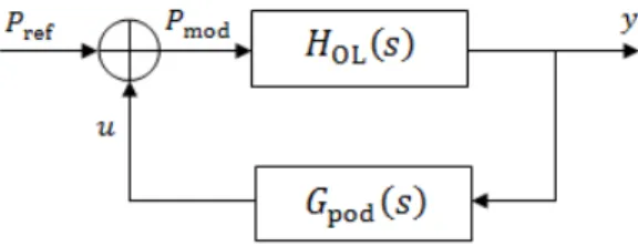
The closed-loop system corresponding to the HVDC link POD control is shown in Fig. 1.
Fig. 1. Closed-loop system with POD controller
As one can see, a supplementary feedback signal u is provided by the POD controller Gpod(s) to modulate the
reference power Pref of the open-loop transfer HOL(s). The
latter represents the power system of Fig. 3 for which the output y is the measure corresponding to the input of the POD. A standard structure of the latter is shown in Fig. 2. It consists of a constant gain K in series with a wash-out filter
Fig. 2. Standard structure of the POD
and lead-lag blocks (see, e.g., [4]). Consider the following decomposition HOL(s) = n X i=1 ri s − λi ,
in which riis the residue of the mode λi. The classical way to
tune the parameters of the POD and to choose its input signal is based on the residues ri (see, e.g., [4]). Indeed, it is shown,
e.g., in [1] that the sensitivity of a mode λi (of the open-loop
system) with respect to the gain K of the POD can be written as
∂λi
∂K = riG1(λi) .
Thus, the shift |∆λi| of the initial mode λi is proportional to
the modulus of the residue ri, since |∆λi| = ∆K|ri||G1(λi) |.
This is why, the appropriate measure is considered as the one which provides the larger modulus of the residue ri
corresponding to the target mode λi for which the damping
has to be improved via the HVDC link. B. Benchmark Structure
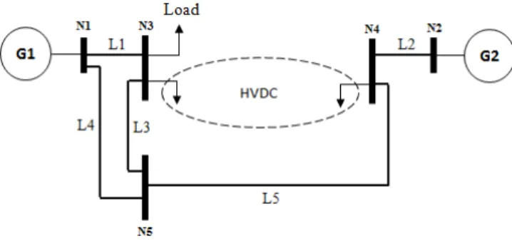
Fig. 3 shows the physical structure of the benchmark pro-posed here to investigate the input signal selection of the POD. It is used to analyse the residues of the inter-area mode in HOL(s) for different local measures y and different structures
and parameters of the system. For this, different impedant pathsbetween the generators and the load are modelled. They are necessary and sufficient to take into account a lot of possible situations and oscillation paths. As a consequence, one can switch from a structure to another one by a simple change of the parameters. For instance, if the length of all the transmission lines is fixed to zero, except the one of L5, one gets the well known benchmark of ‘two generators connected by an HVDC link in parallel with an AC line’. In this way, the residues can be computed for a large number of situations. Also, to simplify the numerical computations, the HVDC link and the generators, used in the benchmark of Fig. 3, are represented by simplified models. For the HVDC link, the so-called injector model (see, e.g., [2]) is used while the generators are both modelled by one axe voltage model (see, e.g., [6]). Their associated voltage and speed regulators are both Proportional-Integral (PI) controllers.
III. INPUT SIGNALS OF THEPOD:RESIDUES BASED ANALYSIS
The procedure proposed here to analyse the effect of the structure and the parameters variation on the choice of the
Fig. 3. Physical structure of the control model
input signal of the POD can be summarized as follows. First, an open-loop transfer HOLi = yi
Pref
is considered for each measure yi available at the connection nodes of the HVDC
link (i.e., local). They are, respectively, the difference of the frequencies y1 = ∆f and voltage angles y2 = ∆θ between
the nodes N3 and N4, the current y3 = I1 though the line
L1 as well as y4 = I2 trough L3 and finally y5 = I1+ I2.
Next, the residue riλ(p) of the inter-area mode λ, which has to be damped via the HVDC link, is computed as a function of the parameters vector p = {z1, · · · , z5, PL}. The
latter are the impedances zi of the transmission lines and
the load power PL while Pref is the reference power of the
HVDC link. Finally, to plot the results, only two parameters are changed simultaneously. They can be either the length of two transmission lines or the load power and the length of a transmission line. Their variation ranges are fixed by grouping together a maximum number of ranges for which the linearised model is stable.
IV. MAIN RESULTS
In this section, the results obtained by the procedure ex-plained above are presented.
A. Case 1 : variation of line length L5 and load power In this first case, the load power PLand the length of the line
L5 are modified in the range [400 1700] (MW) and [1 140] (Km) respectively. The power transmitted by the HVDC link is fixed to 300 MW while the length of all the other lines is equal to zero. Figs. 4 and 5 show the modulus of the residue corresponding to the inter-area mode.
One can first remark the intersection between the surfaces obtained for both measures. This means that the choice of the measured signal depends on the parameters of the system. For medium values of PL (between 400 and 800 MW) and a line
of length more than 50 Km, the measure ∆θ gives residues of lower modulus than the ones provided by (I1+ I2).
Con-versely, when the load power increases, (I1+ I2) provides
residues of greater modulus. In addition, one can also notice that, for the same measure, the modulus of the residue does not increase smoothly and can change a lot for small variations of some parameters in a given range. This is clearly shown in Fig. 5 (e.g., when the length of L5 is around 50 Km). More results are shown bellow to see the effect of the other parameters.
Fig. 4. Difference of angles and sum of currents: first view
Fig. 5. Difference of angles and sum of currents: second view
B. Case 2: length variation of the lines L1 and L2
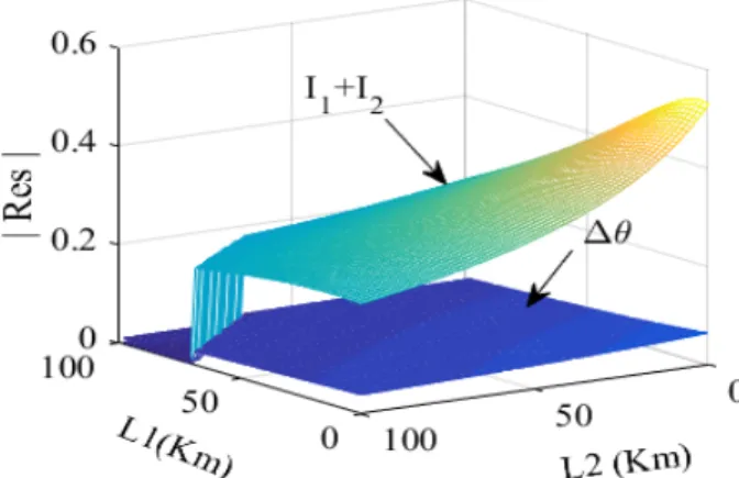
To see the effect of two impedances with different power levels of the system on the modulus of the residue, two situations are considered. In the first one, the load power is fixed to 400 MW while the length of both lines L1 and L2 vary from 1 to 100 Km. In the second one, the same conditions are considered but with a load power of 1500 MW. The length of the other lines L3, L4, L5 are fixed to 0 Km, 1000 Km and 25 Km respectively. For the first situation, the results are shown in Figs. 6.
As in the previous case, on can notice the same kind of non smooth variation of the modulus of the residue. This can be seen in Fig. 6 when the length of both lines is around 100 Km. Moreover, the same figure shows that the modulus of the residue obtained with (I1+ I2) is almost 10 times greater than
the one obtained with ∆θ. Such a result is not preserved in the second situation when PL = 1500 MW. Indeed, in this case
Fig. 7 shows the contrary. For ∆θ, this can be understood since when the load power increases, the magnitude of ∆θ becomes more important explaining the increase of the residue. However, if one consider only the current I1, it can be seen in
Fig. 8, that this leads to a residue of larger modulus than the one obtained for ∆θ. This shows again, that it is not
Fig. 6. Difference of angles and sum of currents: PL= 400 MW
Fig. 7. Difference of angles and sum of current: PL= 1500 MW
obvious to find the appropriate measure without computing and comparing the residue for each of them. In other words, the choice can be done only for known grid situations since it is strongly related to the parameters of the system.
Finally, all these results show that, in the sense of the residues, the appropriate measure to build the POD cannot be chosen a priori. This depends on the situation and on the parameters of the system.
V. USE OF THE PROPOSED BENCHMARK FOR CONTROL PURPOSES
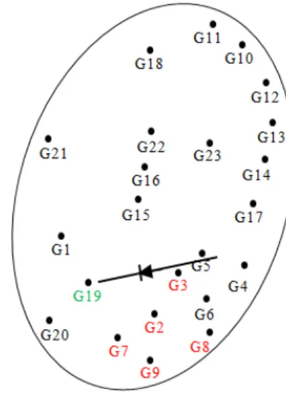
In this section, it is shown how the benchmark presented in Fig. 3 can be used to simplify the analysis and the control of an inter-area mode. The goal is to reproduce the main properties (like frequency, damping and residue) of an inter-area mode of a large-scale power system by tuning the parameters of the benchmark. The way in which this is done is explained below. A. Reference power system
To start, a realistic power system of 23 generators (Fig. 9) is taken as reference for the comparisons. All its generators as well as their associated regulators are modelled in detail. The HVDC link is embedded into the system near the generators G5 and G19. It is used to transport an active power of 400 MW while its nominal active power is 1000 MW. Among all the inter-area modes of the system, the one considered here is mainly between the generators G7, G8, G2, G3, G9, in one side, and G19 in the other side. Its properties are shown in the second column of Table I. The input and the output for which the residue is computed are respectively the active power reference of the HVDC link and the current trough the line represented by L3 in the benchmark of Fig. 3.
B. Comparisons and validation
In order to reproduce the properties of the inter-area mode, described above, with the benchmark of Fig. 3, the first step is to choose two generators among the ones involved in the mode λint mantioned in Section V-A. Here, G7 and G8 are
chosen since they have the largest participations (measured by the modulus of the participation factors, see, e.g., [1]) in λint. Both are used, along with their regulators, in the
benchmark of Fig. 3. In the next step, the values of the load and the length of the transmission lines have to be adjusted. This is done here by trial and error tests but more effective techniques can be envisaged to improve the accuracy of the results. Finally, the properties of the resulting inter-area mode are shown in column 3 of Table I. By comparing with the properties of the original mode (i.e., the one selected from the reference system), one can see that the differences are not too large. This shows the ability of the proposed benchmark to reproduce the properties of an inter-are mode for the purpose of analysis and control. A POD controller is designed, based on the benchmark, and used, in the reference power system, to improve the damping of the considered inter-area mode. The results will be included in the full paper.
VI. CONCLUDING REMARKS
A study on the input selection of the POD controller is presented. For this, a benchmark is firstly proposed to take into account a large number of structures and oscillation paths by simple variation of its parameters. Classes of situations connected to ranges of parameters can thus be given. Next, by systematically considering a wide range of grid situations, it is shown that the choice of an appropriate measure to build the POD cannot be given a priori. More precisely, it is strongly
Fig. 9. Interconnected power system of 23 generators
TABLE I
PROPERTIES OF THE CONSIDERED INTER-AREA MODE
Original inter-area mode Reproduced inter-area mode
Mode (λint) −0.2615 ± j5.3581 −0.3557 ± j6.0884
Frequency (Hz) 0.8528 0.9690 Damping (%) 4.78 5.83
Residue 1.771ej91.8◦ 2.065ej93.5◦
related to the parameters of the system. Especially, the length of the transmission lines and the power level of the system. In other words, there is no a specific measure which can be always the appropriate one. In addition to these investigations, the proposed benchmark is shown useful to analyse and to control an inter-area mode, i.e., as a control model. The validation is done based on a realistic power system of 23 generators.
REFERENCES
[1] G. Rogers, Power System Oscillations. Boston, USA: Kluwer Academic Publishers, 2000.
[2] H. F. Latorre, M. Ghandhari, and L. Soder, “Multichoice control strategy for vsc-hvdc,” in Bulk Power System Dynamics and Control-VII. Revital-izing Operational Reliability, 2007 iREP Symposium. IEEE, 2007, pp. 1–7.
[3] ——, “Use of local and remote information in pod control of a vsc-hvdc,” in PowerTech, 2009 IEEE Bucharest. IEEE, 2009, pp. 1–6.
[4] R. Sadikovic, G. Andersson, and P. Korba, “Damping controller design for power system oscillations,” Intelligent Automation & Soft Computing, vol. 12, no. 1, pp. 51–62, 2006.
[5] E. V. Larsen and J. Chow, “Svc control design concepts for system dynamic performance,” Application of Static Var Systems for System Dynamic Performance, pp. 36–53, 1987.
[6] M. Ilic and J. Zaborszky, Dynamics and control of large electric power systems. Wiley New York, 2000.