HAL Id: tel-02125962
https://tel.archives-ouvertes.fr/tel-02125962
Submitted on 10 May 2019HAL is a multi-disciplinary open access archive for the deposit and dissemination of sci-entific research documents, whether they are pub-lished or not. The documents may come from teaching and research institutions in France or
L’archive ouverte pluridisciplinaire HAL, est destinée au dépôt et à la diffusion de documents scientifiques de niveau recherche, publiés ou non, émanant des établissements d’enseignement et de recherche français ou étrangers, des laboratoires
Investigate the matrix : leveraging variability to
specialize software and test suites
Paul Temple
To cite this version:
Paul Temple. Investigate the matrix : leveraging variability to specialize software and test suites. Software Engineering [cs.SE]. Université Rennes 1, 2018. English. �NNT : 2018REN1S087�. �tel-02125962�
THÈSE DE DOCTORAT DE
L’UNIVERSITE DE RENNES 1
COMUE UNIVERSITE BRETAGNE LOIRE
Ecole Doctorale No601
Mathèmatique et Sciences et Technologies de l’Information et de la Communication Spécialité : (voir liste des spécialités)
Par
Paul TEMPLE
Investigate the Matrix : Leveraging Variability to Specialize Software and
Test Suites
Thèse présentée et soutenue à RENNES, le 7 décembre 2018 Unité de recherche : Equipe DiverSE, IRISA
Thèse No :
Rapporteurs avant soutenance :
Philippe COLLET, Professeur, Université Nice Sophia Antipolis / Université Côtes d’Azur, Nice, FRANCE Myra B. COHEN, Professeur, Iowa State University, Ames, USA
Composition du jury :
Attention, en cas d’absence d’un des membres du Jury le jour de la soutenance, la composition ne comprend que les membres présents
Président : Philippe COLLET, Professeur, Université Nice Sophia Antipolis / Université Côtes d’Azur, Nice, FRANCE
Examinateurs : Philippe COLLET, Professeur, Université Nice Sophia Antipolis / Université Côtes d’Azur, Nice, FRANCE
Myra B. COHEN, Professeur, Iowa State University, Ames, USA Patrick PÉREZ, Directeur Scientifique, Valeo.ai, Paris, FRANCE
Yves LE TRAON, Professeur, Université de Luxembourg, Luxembourg, LUXEMBOURG Mathieu ACHER, Maître de conférences, Université Rennes 1, Rennes, FRANCE
Résumé en français
Contexte
Aujourd’hui, les logiciels sont présents partout autour de nous. On les trouve dans nos téléphones, ordinateurs et toutes sortes d’objets high-tech ; plus récemment, ils se sont introduits directement dans les télévisions, les véhicules, etc. Dans le même temps, ils permettent également de traiter de nouvelles tâches. Leur omniprésence a pour conséquence une hausse des attentes des consommateurs en terme d’efficacité, de performances, etc. En marge de cela, puisque personne n’a les mêmes attentes ni les mêmes demandes, le besoin de personnaliser les logiciels s’est développé.
Malgré tout cela, de nouveaux logiciels continiuent d’être développés chaque jour pour traiter des problèmes qui sont parfois similaires. Par exemple, suivre le ballon durant un match de football ou une voiture de sport lors d’une course ou bien même des personnes piétonnes dans la rue sont autant de tâches exprimées de manière différente. Mais, d’un certain point de vue, en utilisant les bonnes abstractions, nous pouvons voir toutes ces tâches sous le même œil : repérer et suivre des entités. Les tâches précédemment citées sont seulement des instances spécifiques de la plus abs-traite. Cela veut dire que, d’une certaine manière, ces tâches, individuellement, ne prennent qu’une partie de l’ensemble des exigences possibles (par exemple, en ne considérant qu’un champ visuel fixe, avec une caméra qui ne peut pas bouger). Dans le cas plus général des logiciels, cela se traduit par une optimisation particulière : une consommation d’énergie, de mémoire ou de processeur plus basse, un temps d’éxé-cution minimisé ou encore essayer de produire les résultats les plus précis possibles en sont quelques exemples.
L’exemple potentiellement le plus représentatif de logiciels personnalisables (ou configurables) est le noyau Linux qui compte à peu près 13000 options de configu-ration. Si l’on suppose que chacune de ces options ne peuvent être qu’activée ou désactivée, le nombre de combinaisons possibles est de 213000 soit à approximative-ment 103250 possibilités. Dû à ce nombre titanesque, essayer d’exécuter chacune de ces combinaisons dans le but d’évaluer laquelle est la plus appropriée à des besoins définis par l’utilisateur est impossible. Il est donc difficile pour un utilisateur de réussir à trouver au moins une configuration (i.e., une combinaison d’options) qui satisfasse tous ses besoins. De plus, la relation existante entre les options de configuration et les besoins est souvent mal définie ou mal documentée ce qui ajoute de la difficulté à
cette phase de configuration pour l’utilisateur.
Même si l’on met ce problème de côté et que l’on suppose que toutes les confi-gurations peuvent être générées, le temps et les ressources allouées à l’activité de test sont souvent limités, ne permettant d’en exécuter qu’un sous-ensemble et d’en analyser les résultats. Ces résultats sont souvent utilisés pour trouver des bugs dans les programmes mais les besoins exprimés par l’utilisateur peuvent aussi contenir des objectifs de performance (par exemple, le programme doit s’exécuter en un temps in-férieur à un certain seuil, la consommation de mémoire ne doit pas excéder un certain seuil, etc. ). Pour vérifier qu’un programme respecte les besoins de l’utilisateur (que ce soit en terme de performances ou non), plusieurs tests sont souvent nécessaires pour pouvoir observer le comportement du système dans différents contextes d’utilisa-tion. En plus de cela, différents apsects peuvent venir influencer les performances d’un programme. L’utilisation d’oracles (définissant les résultats attendus d’une exécution) devient alors difficile rendant, de fait, l’évaluation de performances délicate. Prenons par exemple le cas d’un encodeur vidéo, ses perfromances (e.g., le temps d’exécution ou la qualité de la vidéo en sortie) peuvent dépendre de la vidéo d’entrée elle-même : la vidéo peut être de mauvaise qualité avec du bruit, ce qui la rend difficile à encoder correctement (diminuant la qualité en sortie) ou bien un algorithme pour enlever le bruit peut être ajouté dans le processus de traitement mais cela augmentera le temps d’exé-cution comparé à d’autres exéd’exé-cutions qui ne nécessitent pas l’ajout de cet algorithme. Au final, il faut prendre en compte deux dimensions distinctes : tout d’abord, la phase de configuration du système qui consiste à sélectionner des options et à leur donner des valeurs ; et également sélectionner des cas de tests, pertinents pour une tâche, qui permettent d’observer les comportements des programmes, générés par la dimension précédente, dans des conditions différentes rendant possible de définir si un système respectent les besoins utilisateurs.
Dans cette thèse, nous représentons ces deux dimensions comme une matrice. Une dimension représente les systèmes que l’on génère grâce à la phase de configu-ration tandis que l’autre dimension représente l’ensemble des cas de tests qui seront exécutés sur chacun des systèmes. De ce fait, chaque cellule représente l’exécution d’un programme particulier sur un cas de test donné et l’on y reporte les performances observées. Dans le cas général, plusieurs performances peuvent être observées lors d’une seule exécution afin de décider si le système respecte bien tous les besoins de l’utilisateur, la celllule peut alors être représentée sous la forme d’un vecteur.
Programmes Cas de tests
Programme 1 Programme 2 ... Programme N
Test 1 12 1 ... 5
Test 2 1 348 ... 10
...
Test M 50 101 ... 260
FIGURE 1 – Un exemple de matrice de performance exploitée dans cette thèse.
Chaque cellule est le résultat d’une exécution d’un programme (colonne) sur un cas de test (ligne). Dans cet exemple le temps d’exécution a été mesuré et reporté dans les cellules de la matrice exprimé en secondes.
La figure 1 donne un exemple de représentation de cette matrice. Dans cet exemple, les colonnes représentent différents programmes (réalisant tous la même tâche mais avec des paramètres différents) à comparer pour que l’utilisateur final puisse choisir celui qui lui convient le mieux alors que les lignes représentent les différents cas de test à exécuter qui sont représentatifs de l’environnement dans lequel le programme sera plongé pour réaliser sa tâche. Pour chaque exécution, le temps d’exécution est mesuré (en secondes) et reporté dans la cellule adéquate de la matrice.
Nous nous intéressons à cette matrice car une simple analyse des valeurs reportés dans les cellules montre déjà un certain intérêt :
— Le programme 1 a l’air plutôt stable sur l’ensemble des cas de tests car il produit des temps d’exécution qui ont l’air relativement bas (moins d’une minute) par rapport à d’autres exécution ;
— Le premier cas de test a l’air relativement simple à traiter puisque les valeurs rapportées sur la première ligne sont très basses (quelques secondes unique-ment) ;
— Le second cas de test semble difficile pour le second programme la valeur cor-respondante étant élevée (plusieurs minutes).
On a donc une analyse qui prend en compte les deux dimensions (soit de manière indépendante soit les deux à la fois). Cette première analyse est donc intéressante que ce soit du point de vue des logiciels (les paramétrisations des logiciels peuvent être mises en relation avec les performances ce qui peut aider du point de vue de la sélection du programme adéquat) ou du testeur (puisque les variations de performance des différents programmes peuvent être observées pour un cas de test donné ce qui peut soulever par la suite des interrogations et des analyses plus poussées).
Contributions
Cette thèse prétend que cette matrice de performance est un concept fondamental qu’il faut exploiter car elle apporte des informations essentielles que ce soit du point de vue de la pertinence des cas de tests utilisés ou du point de vue de la performance des programmes à comparer. Dans les mains d’ingénieurs du logiciel, cette matrice devrait permettre de réaliser différentes tâches utiles (que ce soit pour améliorer des logiciels existants mais aussi dans les phases de test avant production etc. ).
Dans cette thèse, deux contributions principales sont mises en avant.
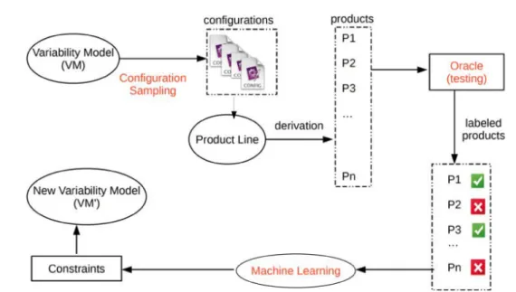
Tout d’abord, le problème de configuration et de sélection d’une configuration est difficile dû au nombre gigantesque de possibilités que les logiciels modernes proposent grâce aux options de configuration. Malheureusement, pour l’utilisateur final, c’est sou-vent un sous-ensemble de cet immense espace de configuration qu’il est nécessaire d’analyser afin de trouver une paramétrisation suffisante pour réaliser une tâche spé-cifique sous certaines conditions. Une pratique commune est alors de tester une pa-ramétrisation (aussi appeler configuration) d’un programme et de voir si elle convient ou pas, si ce n’est pas le cas, il faut changer la valeur des paramètres et recommen-cer jusqu’à réussir. L’utilisateur se retrouve donc un processus de sélection basé sur l’essai-erreur. Dans le meilleur des cas, l’utilisateur va trouver en quelques essais une configuration qui lui convient, dans le cas contraire, il faudra plus d’essais. Un autre aspect a prendre en compte est que la paramétrisation peut prendre un certain temps (par exemple, dans le cas où le système doit être recompilé), dans ce cas, même quelques essais peuvent être chronophage et énergivore ce qui n’est pas désirable. Notre but est donc de réussir à réduire cet espace de configuration en amont afin que l’utilisateur est un nombre moindre de programmes à prendre en compte. Nous pro-posons d’utiliser une technique d’apprentissage automatique afin de réaliser cette ré-duction. A partir d’un sous-ensemble de programmes, d’exécutions sur des cas de test ainsi qu’une fonction oracle qui réfère aux besoins de l’utilisateur. Le principe est alors d’utiliser l’oracle sur les résultats des exécutions afin d’apposer un label définissant si le programme (ou plus précisemment sa paramétrisation) doit être gardée dans l’en-semble des programmes qui peuvent être utilisés par l’utilisateur final ou non. Une fois toutes ces exécutions annotées, l’algorithme d’apprentissage automatique peut créer une fonction séparatrice entre les paramétrisations à garder et les autres afin de ré-duire automatiquement l’espace de configuration. Grâce à l’approche statistique et au pouvoir de généralisation de l’algorithme d’apprentissage automatique, cette approche
permet d’écarter un certain nombre de configurations tout en gardant les programmes avec un fort potentiel d’adéquation aux critères de l’utilisateur. Un problème subsis-tant est alors de ne pas faire trop d’erreurs de classification ce qui pourrait réduire les possibilités de configuration de l’utilisateur plus que nécessaire ou au contraire ne pas être capable d’écarter assez de configurations ce qui reviendrait au processus d’essais-erreurs initial. Cette première contribution vise donc à réduire la première di-mension de notre matrice de performance. Nous validons cette approche sur différents systèmes, notamment un générateur de séquence vidéos.
La seconde contribution majeure de cette thèse est une nouvelle méthode qui vise à évaluer la capacité de suites de tests à révéler des différences significatives dans les performances des différents programmes qui réalisent une même tâche. En effet, le temps et les ressources alloués à l’activité de tests étant limités, il est nécessaire de réduire au maximum le nombre d’exécutions à réaliser et donc il faut pouvoir proposer un nombre de cas de tests suffisant mais minimal afin d’optimiser cette activité. Le pro-blème est que le choix des cas de tests à utiliser reste un propro-blème ardu. Par exemple, les banques de données d’images utilisés dans les compétitions d’algorithmes de re-connaissance d’objets sont de plus en plus grandes ce qui allongent le temps de cal-cul et qui désavantages les compétiteurs qui ne peuvent pas se permettre d’avoir de grosses puissances de calcul ; mais est-ce que toutes ces images sont vraiment néces-saires ? Ne peut-on pas réduire ces données de tests tout en conservant la capacité de l’ensemble de tests à discriminer les compétiteurs ? Dans ce contexte, une suite de tests nous paraît intéressante si elle est capable de donner une vue d’ensemble des performances des programmes que l’utilisateur pensent pouvoir utiliser. Ainsi, il est nécessaire de garder dans cette suite de tests des cas de tests qui sont capables de montrer que, par exemple, ils ont été traîtés de manière beaucoup plus longues que d’autres par certains programmes, ce qui peut être décisif dans le cas où le pro-gramme est plongé dans un environnement où il nécessite de répondre en temps réel. Dans cette contribution, nous introduisons la notion de "couverture de performance". Pour mesurer cette couverture, nous proposons d’utiliser le score de dispersion. Il se construit sur la base d’un histogramme qui va permettre de séparer le domaine de définition d’une performance donnée en plusieurs sous-domaines disjoints. Le but est qu’au moins une exécution permette de peupler chaque sous-domaine. Plus le nombre de sous-domaine représenté est élevé, plus la suite de tests est considérée comme étant intéressante et devrait être conservée puisqu’elle permet d’observer différents
comportements provenant de différents programmes. Cette approche a été évaluée sur différents domaines d’applications et nos résultats montrent d’une part l’efficacité du score de dispersion tel que nous l’avons défini pour conserver des suites de tests qui semblent plus intéressantes que d’autres et d’autre part la possibilité d’utiliser cette approche pour différentes tâches comme par exemple réduire un ensemble de suite de tests ou encore mettre en avant des comportements de programmes qui semblent "bi-zarres" (i.e., déviants par rapport au reste de l’ensemble des programmes considérés) ce qui permet de pousser l’analyse plus loin pour peut-être découvrir des bugs dans le code. Cette deuxième contribution s’attaque donc tout d’abord la deuxième dimension de notre matrice de performances. En évaluant la qualité des suites de tests, il est possible par la suite d’optimiser la phase d’exécution en réduisant le nombre de tests à exécuter ou en donnant un ordre (par exemple, ceux qui ont un score de dispersion plus élevé d’abord).
Au final, nos contributions visent à réduire l’une ou l’autre des deux dimensions présentées par la matrice de performances permettant par la suite d’avoir un choix res-treint mais toujours pertinent pour la suite du processus de génération de programmes ou de tests.
Abstract
Nowadays, software have to be efficient, fast to execute, etc. They can be confi-gured in one way or another to adapt to specific needs. Each configuration leads to a different system and usually it is hard (if not impossible) to generate them all. Thus, the exhaustive evaluation of their performance is impossible. However, a single user has specific requirements and needs to find an appropriate configuration of a system. To ensure the adequacy between performances and requirements, several executions under different conditions are needed adding computation time to the daunting task of selecting a proper configuration.
Two dimensions emerge from this description of performance testing : the selection of relevant system configurations that influence the behavior of associated system and the selection of test cases allowing to observe performances of systems under different conditions.
We propose to represent those two dimensions as a (performance) matrix : one dimension represents selected systems for which performances can be observed while the other dimension represents the set of test cases that will be executed on each of these systems. Each cell is the execution of a program variant regarding a test.
The contributions of this thesis are as follows :
First, we leverage Machine Learning techniques in order to specialize a Software Product Line (in this case a video generator) helping the selection of a configuration that is likely to meet requirements. End users must be able to express their require-ments such that it results in a binary decision problem (i.e., configurations that are acceptable and those that are not). Machine Learning techniques are then used to re-trieve partial configurations that specialize a Software Product Line to guide end users and reduce the configuration space. In the end, this work aims at diminishing the first dimension of the matrix that deals with systems and programs.
Second, we propose a new method assessing the ability of test suites to reveal significant performance differences of a set of configurations tackling the same task. This method can be used to assess whether a new test case is worth adding to a test suite or to select an optimal test set with respect to a property of interest. In the end, it may help structuring the execution of tests. For instance, it can create an order of execution resulting in using less test cases that are presented in the second dimension of the matrix. We evaluated our approach on several systems from different domains
A
CKNOWLEDGEMENTS
First, I would like to thank very warmly the members of the jury for accepting to review the work I have conducted during the past three and a half years. This PhD was a big step in my life and having such encouraging comments and relevant questions coming from such a panel of researchers was way out of my consideration for a long time. I would like to thank Prof. Philippe Collet for having taken the chair of this jury. Having you, a mentor of one of my supervisor, in this jury was very challenging for me considering that I knew very little about configurable systems a few years ago. Thank you to Prof. Myra Cohen for accepting to listen to me despite it was very early over there. Your comments and enthusiasm were very heart-warming. Thank you Prof. Yves Le Traon for the every now and then talks we had during these three years and for showing your interest in my work. Thank you very much to Patrick Pérez for being the only representative (in this jury) of the image processing community. We have met several times during this PhD, you were always careful about what I was presenting and you were of great advice despite being so much busy. Furthermore, you were constantly reminding me how interesting the ideas we were talking about could benefit to industries giving me full of energy every time we met.
I would like to thank my former teachers who taught me everything I know about video and image processing but also machine learning, computer graphics and much more. From IUT to the ESIR, thank you all Pierre, Philippe, Adib, Sébastien, Kadi, Rémi, Fabrice and the others.
Ewa and Laurent you were excellent advisers during my internship at TEXMEX some years ago. You taught me so much during these few months about research in general but also the level of expectation that I needed to reach to be an excellent re-searcher. In addition, you introduced me to the security problems in Machine Learning and put me in touch with Battista. I am very grateful to both of you for all of that.
Guillaume, you told me about configurable systems more than 5 years ago now, almost immediately we talked about how similar this domain and research in machine learning can be. This talk has driven my research and you were also the one telling me about this PhD opening in DiverSE. I want to thank you very warmly for this.
While it was very hard for me to get anything from the first talks during breaks or meetings, the atmosphere inside DiverSE always remained excellent. I want to say thank you DiverSE (present and past members) for being so kind, curious (about my knowledge) and understanding about the fact that not everybody knows software engi-neering (even if you think that this is a big mistake) and to Olivier and Benoît for leading the team. José, you were the person that put me on track and I am very pleased I was able to work with you ; I must have been a pain in the butt during this first year when I hardly knew anything about the stack behind variability, configurations, etc. You have always been there to help me being very calm and willing to share your knowledge. Thank you Pierre, Kévin, Fabien, Marcellino, Alejandro and Oscar for the all the mo-ment we shared (about work but also the others). Special thanks to Johann with whom I could always talk about tennis (even if I was disturbing you). Tifenn, we arrived at the same time in the team, we were two costarmoricans in this foreign country that is Rennes. You were also there to talk about anything but work, I really appreciated all these moments with you. Caroline, DiverSE is lucky to have you, you are kind of the "mom" of the team, thank you for everything.
Of course, Jean-Marc and Mathieu ! Thank you very much for giving me the op-portunity to work with you. You were tremendous supervisors despite your very busy schedules. Of course, I learnt a lot from your scientific guidance. Brainstorming ses-sions were exhausting to me, yet, a lot of ideas, new directions long terms vision came out of these. I am glad to know that the work I have begun will continue in the team un-der your supervision and that somehow we started a new focus in the team. Apart from that, you were always there when I needed explanations, when I was feeling uncom-fortable or when I did not know where to go ; you always took one hour or more to talk about all these problems and I cannot emphasize enough how much it was important to me.
I am very proud of what I did at work, but I could not have accomplished that without all the people I met outside the lab. The TCTF is the best tennis club I have ever seen. I met a lot of people willing to play tennis just as much as I do. Thank you to all the partners and teammates. Olivier B. you are the best trainer ever ! From the first hour of training (in groups) to the last (in individual), you made far better than I could have ever imagined. All those hours with you on the court improved my focus and my endurance which were beneficial in my work. Thank you very much for everything. I hope you will keep giving this good energy that you give to people and that you will be able to share
your passion with people for a long time.
M’man and Pierre... When I started my PhD, things were a bit complicated between us : "why do you work that much ? Why do you work that late ?" were common questions I heard every now and then. I think you know now why I did this. However, as the thesis kept going, you were there to cheer me up, to comfort me and support me constantly. This is also thank to both of you that we have a doctor in the family now.
Finally, to you, the person I met 8 years ago in Lannion. The three past years were not easy for us. Despite all of this, you were the person that kept me alive, pushing me to take vacations when I was exhausted and could not think straight a few weeks before deadlines. You were there no matter what, even when you were just as exhausted as I was. I think you lived this PhD like you were actually doing a PhD. I am sorry for the hard time I made you live (and also for the numerous upcoming ones as long as we stay together). I love you Marine.
R
EMERCIEMENTS
Tout d’abord, je voudrais remercier très chaleureusement les membres du jury qui ont accepté de rapporter et d’évaluer les travaux que j’ai mené durant ces trois der-nières années et six mois. Cette thèse a été un moment très important dans ma vie et le fait d’avoir reçu ces commentaires encourageants et des questions aussi pertinentes provenant de ces personnes m’a toujours paru hors de portée. Je souhaiterai remer-cier Philippe Collet pour avoir accepter de présider ce jury. Vous avoir vous, un mentor d’un de mes propres encadrants, dans ce jury a été très particulier pour moi surtout en sachant que je ne connaissais pratiquement rien aux systèmes configurables il y a quelques années de cela. Merci à vous, Myra Cohen pour avoir accepter de m’écouter alors qu’il était très tôt aux Etats-Unis. Vos commentaires et votre enthousiasme m’ont été très réconfortant. Merci à Yves Le Traon pour avoir montré autant d’intérêt à mes travaux et pour les discussions que nous avons eu pendant ces trois ans. Patrick Pé-rez, merci beaucoup d’avoir été le seul membre de ce jury a être le représentant de la communauté du traitement de l’image. Nous nous sommes rencontrés régulièrement durant cette thèse, vous avez toujours su vous montrer d’une écoute particulièrement attentive, vous m’avez été de précieux conseils et tout ça même en étant extrême-ment débordé. En plus de cela, vous m’avez toujours rappelé à quel point les idées que j’avais pouvais être intéressantes pour le monde de l’industrie, me redonnant à chaque fois de l’énergie pour continuer.
Je voudrais également remercier mes enseignants qui m’ont tout appris au sujet du traitement de l’image et de la vidéo mais également tout ce qui traite du machine learning, la synthèse d’images et plein d’autres choses. Depuis l’IUT jusqu’à l’ESIR, merci à Pierre, Philippe, Adib, Sébastien, Kadi, Rémi, Fabrice et tous les autres.
Ewa et Laurent, vous avez été d’excellents maitres de stage pendant mon séjour à TEXMEX, j’ai été extrêmement fier d’avoir pu travailler avec vous. Vous m’avez appris tellement, pendant ces quelques mois, sur la recherche en général mais également sur le niveau d’éxigence que je devais atteindre si je voulais être bon dans ce que je fais. En plus de ça, vous m’avez aussi fait connaitre les problèmes de sécurité liés au machine learning et j’ai pu, grâce à vous, être en contact avec Battista, je vous suis
très reconnaissant pour ça.
Guillaume, tu as commencé à me parler des systèmes configurables il y a 5 ans à peu près, très rapidement nous avons parlé des similitudes qu’il existait entre ce do-maine et celui du machine learning. Cette discussion m’a guidé régulièrement pendant cette thèse et tu m’as également mis au courant que DiverSE recherchait un candidat pour une thèse au parfait moment. Je veux te remercier énormément pour ça.
Même si il a été très difficile pour moi de comprendre quoi que ce soit aux pre-mières pauses et premiers meetings, l’atmosphère au sein de DiverSE a toujours été excellente. Je remercie beaucoup DiverSE (membres présents et passés) pour avoir été si gentil, curieux (sur mon parcours et ce que je pouvais apporter à l’équipe) et compréhensif sur le fait que tout le monde ne connaisse pas vraiment le génie logiciel (même si, à priori, c’est une énorme bêtise) et à Olivier et Benoît pour organiser cette équipe. José, tu m’as guidé au tout début et j’ai été très heureux d’avoir pu travailler avec toi ; j’ai pourtant dû être une vraie plaie pendant ma première année, quand je ne connaissais pratiquement rien à tout ce qui touchait à la variabilité, aux configura-tions et tout ça. Tu as toujours été présent pour m’aider et tu as su toujours partager tes connaissances. Merci à Pierre, Kévin, Fabien, Marcellino, Oscar et Alejandro pour tous les moments partagés (boulot et autres). JMerci également à Johann avec qui je pouvais toujours parler tennis (même si je sentais que je le dérangeais). Tifenn, on est arrivé au même moment dans l’équipe, nous étions les deux costarmoricains dans ce pays très lointain qui est Rennes. Tu étais toujours là pour parler de tout sauf du travail, ça m’a fait énormément de bien. Caroline, DiverSE peut être vraiment content de t’avoir, tu es un peu la "maman" de l’équipe, merci pour tout.
Bien sûr, il y a aussi Jean-Marc et Mathieu ! Merci énormément pour m’avoir permi de travailler avec vous. Vous avez été tout simplement exceptionnels en tant que di-recteur et encadrant bien que vous aviez un emploi du temps bien chargé à côté. J’ai appris tellement de choses grâce à vous et votre sens de la recherche. Les sessions de brainstorming ont été très éprouvantes pour moi au début, mais, il en ressortait toujours tout un tas d’idées, des nouvelles directions à explorer et des visions à long-terme. Je suis très fier de savoir que le travail que j’ai commencé va se poursuivre au sein de l’équipe à vos côtés, mais je suis également fier du fait que l’on est pu commencé, en quelque sorte, un nouvel axe de recherche. En plus de tout ça, vous avez toujours su être là quand j’avais besoin d’explications ou de conseils, quand je me posais tout un tas de questions ; vous avez toujours pris du temps pour parler de
tout ça et je n’ai pas les mots pour vous dire à quel point ça a été important pour moi. Je suis très fier du travail que j’ai accompli, mais je n’aurais pas pu terminer tout ça sans les personnes qui étaient là en dehors du labo. Le TCTF est le meilleur club que j’ai connu. J’y ai rencontré des tas de personnes qui ont toujours au moins tout autant motivées que moi pour jouer. Merci à tous mes partenaires de jeu et aux co-équipiers. Olivier B., tu es au top ! Du premier entrainement (en groupe) jusqu’au dernier (en in-div), tu m’auras fait devenir bien meilleur que ce que je n’aurais pu imaginer. Toutes ces heures passées avec toi auront également amélioré ma concentration et mon en-durance ce qui aura été très bénéfice pour le travail. Merci énormément ; j’espère que tu réussiras à garder l’énergie que tu transmets et que tu pourras continuer à partager ta passion pendant encore longtemps.
M’man et Pierre... Quand j’ai commencé ma thèse, ça n’a pas toujours été facile pour nous : "Pourquoi tu travailles autant ? Pourquoi tu restes aussi tard ?" ont été des questions récurrentes. Je pense que maintenant vous comprenez pourquoi. Au fur et à mesure que la thèse avançcait, vous avez toujours été là pour moi. C’est aussi grâce à vous 2 que nous avons un docteur dans la famille.
Pour terminer, à toi la personne que j’ai rencontré il y a 8 ans à Lannion. Les trois dernières années n’ont pas été faciles pour nous. Malgré tout cela, tu as été la per-sonne qui m’a fait survivre, en me forçant à prendre des vacances quand j’étais totale-ment exténué et que je n’arrivais plus à réfléchir alors que des deadlines arrivaient. Tu étais là, tous les jours, même quand toi-même tu n’en pouvais plus. Au final, je pense que tu as vécu cette thèse tout autant que moi. Désolé pour tous les mauvais moments que je t’ai fait vivre (et aussi pour les prochains à venir). Je t’aime Marine.
T
ABLE OF
C
ONTENTS
Résumé en français 3
Abstract 9
1 Introduction 20
2 Background 25
2.1 Software Product Lines . . . 25
2.1.1 Perks of reuse . . . 25
2.1.2 SPL development process . . . 26
2.2 Feature Models . . . 29
2.2.1 Fundamentals of feature models . . . 30
2.3 Machine Learning . . . 34
2.3.1 Stages to use a machine learning algorithm . . . 36
2.3.2 The training phase . . . 37
2.3.3 Evaluating prediction performances . . . 38
2.3.4 Overfitting and underfitting . . . 39
2.3.5 Hyperparameters and validation set . . . 40
2.4 Summary . . . 41
3 State of the Art 43 3.1 Software product lines and Testing . . . 44
3.1.1 Configuration sampling . . . 44
3.1.2 Fault Detection in software product lines . . . 46
3.1.3 Metamorphic Testing . . . 48
3.2 Tests quality . . . 49
3.2.1 Traditional metrics . . . 49
3.2.2 Mutation Testing . . . 50
3.2.3 Quality of performance tests . . . 51
TABLE OF CONTENTS
3.3.1 Performance prediction . . . 51
3.3.2 Testing machine learning techniques . . . 53
3.4 Summary . . . 54
4 Automatic Specialization of software product lines using Machine Lear-ning 57 4.1 Introduction . . . 57
4.2 Method . . . 60
4.3 Case Study . . . 64
4.3.1 Case and Problem . . . 64
4.3.2 Solution for Inferring Constraints . . . 65
4.3.3 Generating a training set out of the variability model . . . 66
4.3.4 Oracle . . . 67 4.3.5 Machine learning . . . 67 4.3.6 Extracting constraints . . . 68 4.4 Experiments . . . 71 4.4.1 Experimental Setup . . . 71 4.4.2 Results . . . 71 4.4.3 Threats to validity . . . 77 4.5 Discussions . . . 79 4.6 Conclusion . . . 81
5 Learning-based Performance Specialization of Configurable Systems 83 5.1 Introduction . . . 83
5.2 Motivation and Problem Statement . . . 85
5.2.1 Motivating scenario . . . 85
5.2.2 Approach . . . 87
5.2.3 Novel problems . . . 88
5.3 Discussions . . . 90
5.3.1 Impacts of performance objectives on the learning problem . . . 90
5.3.2 Measures to assess the prediction power of machine learning models . . . 91
5.4 Experiments . . . 94
5.4.1 Subject systems and configuration performances . . . 94
TABLE OF CONTENTS
5.4.3 Presentation of results . . . 96
5.4.4 RQ1) Does our method allow to accurately classify configurations ? 96 5.4.5 RQ2) Does our method allow to maintain flexibility while being safe ? . . . 103 5.5 Conclusion . . . 110 6 Multimorphic Testing 113 6.1 Introduction . . . 113 6.2 Multimorphic Testing . . . 116 6.2.1 Motivation . . . 116
6.2.2 The principle of Multimorphic Testing . . . 117
6.2.3 Properties of a measure . . . 118
6.2.4 Design of dispersion measures . . . 119
6.3 Empirical Evaluation . . . 123
6.3.1 Research questions . . . 123
6.3.2 Evaluation settings . . . 123
6.3.3 RQ1 : Is the dispersion measure right ? . . . 128
6.3.4 RQ2 : Is the dispersion score a right measure ? . . . 132
6.3.5 Concluding remarks over the method . . . 137
6.3.6 Reproducibility of experiments . . . 138
6.4 Discussions and Threats to Validity . . . 139
6.4.1 Internal threats . . . 139
6.4.2 External threats . . . 139
6.5 Conclusion . . . 142
7 Conclusion and Future Work 143 7.1 Conclusion . . . 143
7.2 Perspectives . . . 144
7.2.1 Machine Learning, Variability and Software Product Lines . . . . 144
7.2.2 Developing an appropriate sampling method . . . 146
7.2.3 Adversarial Machine Learning and Software Product Lines . . . 147
7.2.4 Taking into account the surrounding context . . . 148
CHAPITRE 1
I
NTRODUCTION
People are nowadays more and more demanding regarding the characteristics of their software. They want software to be efficient, fast to execute and sometimes even able to optimize several different aspects at once. In the meantime, software are taking evermore importance in our daily activities : they are in our computers and smart-phones ; for a few years now, they are helping us driving cars, etc. As the number of programs increases, they tackle new problems that are more and more complex. Yet, different software continue to be independently created to tackle similar tasks. For ins-tance, tracking a ball in soccer games or cars in races or even tracking people in the street might all seem different (because it does not aim to track the same entity) howe-ver, at a certain level of abstraction, all of them track entities. Their differences come from the fact that they take into account only a subset of users’ requirements but not all at once. Some are optimized to consume less memory, others are tuned to produce the most accurate results, etc.
One representative example of software trying to cope with different users’ requi-rements is the Linux Kernel which contains about 13, 000 options. Assuming that all options can only be activated or deactivated, the number of combinations of options is up to 213,000 or about 103,250 possibilities. This number is so big that it is impossible to review them all exhaustively in order to find which ones suit pre-defined requirements. Thus, it is hard for users to choose and find a proper configuration (i.e., combination of options) that complies with their requirements. Finding such a configuration is usually difficult as the mapping between options and requirements is not straightforward and the documentation might not reflect properly on how an option affects the behavior of the program.
Even if all configurations of a system can be generated, time and resource budgets conferred to the testing activity permit to generate only a few of them, restricting the observation of performances to resulting programs. Besides the task of finding bugs in systems, requirements might express some performance goals (e.g., run under a
cer-Introduction
tain amount of time, use at most a certain amount of memory). Usually, to assess that a given program complies with requirements (being related to performances or not), several tests are needed to observe the system under different conditions. Further-more, because different aspects can influence performances, the definition of oracles (or expected results) can be difficult, making the assessment of performances tricky. For instance, considering a video encoding algorithm, its performances (e.g., its exe-cution time or the quality of the output video) might depend on the input itself : if the video is of poor quality, with dynamic noise, it might be hard to encode correctly or a denoising algorithm can be used in the pipeline of the encoder resulting in an increase in its execution time compared to other executions without this additional step.
In the end, two dimensions emerge : first, configuring a system which consists in se-lecting options and assigning them a value ; and, second, sese-lecting relevant test cases that will allow to observe the behavior of generated systems under various conditions in order to know whether they will meet requirements. We propose to represent those two dimensions as a (performance) matrix : one dimension represents selected sys-tems for which performances can be observed while the other dimension represents the set of test cases that will be executed on each of these systems. Each cell is the execution of a program variant regarding a test. In the general case, a cell might be a vector as multiple measures being observed at the same time and needed to decide whether a system meets requirements. Figure 1.1 illustrates how we represent this matrix. In this example, columns represent program variants and rows represent test cases of a test suite to execute. Let us consider that for each execution, the execution time is measured (in seconds) and reported in cells of the matrix. Based on this matrix, we can say a few things :
— Program 1 seems to be rather stable, providing rather low execution times (less than a minute) ;
— Test Case 1 seems to be easily handled by most of the Program Variants ; — Test Case 2 seems to be difficult for Program 2 which shows a high value. All of these analyses are interesting either from the software system point of view (as we can map configurations to performances) or from the test suite point of view (as we can observe the diversity of performance results with regards to a test case).
This thesis claims that performance matrices are a fundamental concept that brings interesting information regarding execution of tests and program variants and thus should be leveraged by software engineers for several very useful tasks.
Introduction
Program Variants Test cases
Program 1 Program 2 ... Program N
Test 1 12 1 ... 5
Test 2 1 348 ... 10
...
Test M 50 101 ... 260
FIGURE1.1 – An example of the performance matrix we exploit in this thesis. Each cell is the result of the execution of a Program Variant (columns) with a Test case (rows). Let us consider that execution time is measured and expressed in seconds.
Contributions :
First, we leverage machine learning techniques in order to specialize a configurable system. The goal is to help selecting a configuration that is likely to meet requirements. In this context, machine learning will use a set of available configurations to predict whether a specific configuration is likely to meet user-defined requirements. End users must be able to express their requirements such that it results in a binary decision pro-blem (i.e., configurations that are acceptable and those that are not). Machine learning techniques are then used to retrieve partial configurations that specialize a configu-rable system to guide end users and reduce the configuration space. In the end, it aims at diminishing the first dimension of the matrix that deals with systems and pro-grams. We validate this approach with a case study (a video generator) and answer the following research questions : i) can we extract constraints from the machine learning technique that actually make sense ? ; ii) are machine learning techniques accurate in their prediction regarding the fact that a product is able to meet users’ requirements ? ; iii) analyzing pros and cons of the proposed approach.
Second, we propose a new method assessing the ability of test suites to reveal significant performance differences of a set of configurations tackling the same task. More precisely, we propose a framework defining and evaluating the coverage of a test set with respect to a quantitative property of interest, such as the execution time or the memory usage. This framework can be used to assess whether a new test case is worth adding to a test suite or to select an optimal test set with respect to the property of interest. In addition, this technique might help structuring the execution of tests. For instance, it can create an order of execution resulting in using less test cases that are presented in the second dimension of the matrix. We validate this new method on three different case studies and answering the following research questions : i) is our new
Introduction
measure used to evaluate test suites right ? Meaning that, does it reflect on the fact that test suites can be discriminated ? And is the measure stable ? ; ii) are new test suites (created by optimizing our measure) efficient ? In other words, is a test suite with a higher score better than an other one with a lesser score ?
Figure 1.2 shows rather intuitively how these contributions interact with the perfor-mance matrix. The second contribution does not appear on Figure 1.2 as we presented
FIGURE 1.2 – Our two contributions in perspective of the performance matrix it as an extension of the first contribution focusing on a specific aspect (i.e., the defini-tion of users’ requirements) and their impact on the performances of machine learning. The remaining of this thesis is structured as follows : Chapter 2 gives the main concepts related to software product lines, variability models and machine learning. In particular, we give the main motivation to use software product lines and software reuse, we focus on a specific kind of variability models called feature models and we finally present basics concepts behind machine learning.
Chapter 3 gives an overview of previous works that have been conducted in the field of testing program variants, test suite optimization, performance evaluation and quality of tests.
Chapters 4 to 6 detail the contributions of this thesis. Chapter 7 concludes and discusses future works.
CHAPITRE 2
B
ACKGROUND
2.1
Software Product Lines
With today’s mass customization industry, the traditional software engineering deve-lopment process has changed [54, 55, 74]. From building one single piece of software answering requirements of a single user, it has come to the point where multiple similar software systems are developed from a common base of code [53, 61].
Clements et al. [21] gives the following definition of a software product line :
Definition 1 (Software Product Lines) A software product line is a set of
software-intensive systems sharing a common, managed set of features that satisfy the specific needs of a particular market segment or mission and that are developed from a com-mon set of core assets in a prescribed way.
Definition 1 shows two aspects of the code of software product lines : a common part and a "variable" part that answers specific needs. Common parts by definition are shared by all products while "variable" parts are present only in certain products.
2.1.1
Perks of reuse
Today’s software are getting bigger and more complex in terms of customization possibilities. As an example of customizable software, the Linux Kernel [21, 60, 91] is probably the most complex piece of configurable software ever created with more than 13, 000 configuration options. With such a number of options, it is difficult to keep a clear view of the structure of the system.
Pohl et al. [74] state the following benefits from reusing as many pieces of code as possible :
— reducing development cost ; — reducing time-to-market ;
Partie , Chapitre 2 – Background
— improving code quality.
Since reuse is at the heart of software product lines, developers have to think carefully about the structure of their code. Capitalizing on code reuse is a way to reduce the amount of code to develop by integrating already existing pieces in new software. With less functionalities to be developed, new products (e.g., software or systems) can be ready and accessible to customers more quickly. Finally, with variability, the structure of code changes (e.g., with parameters and options activated at run-time or ifdef ins-tructions at compile time). Since links are made between code and functionalities, it can be easier to target specific parts of code in which a bug have been detected. Also it results in fixing the bug at one place while being applied to every products that share the modified piece of code. Since different functionalities can be split among several options, ifdefs and if conditions at different places in the code, code become harder to read and its flow might be broken making it harder to follow and understand.
In the end, commonalities are conceived only once ; remaining parts of the code (i.e., variable or optional parts being specific to some requirements) are decoupled and built such that they can be combined to generate the desired software.
Nowadays, software embed so much variable aspects that they are depicted as variability intensive systems [29, 70].
Svahnberg et al. [95] defines software variability as follows :
Definition 2 (Variability) Software variability is the ability of a software system or
artifact to be efficiently extended, changed, customized or configured for use in a par-ticular context.
As software variability becomes omnipresent (e.g., in video encoding, machine lear-ning techniques, operating systems, code generators, etc. ), the number of products to manage increases quickly and becomes out-of-hand.
Hence, it can be hard to keep track of implemented functionalities and where can be found in the code or, the other way around, what are the parts of the code that are impacted by a certain functionality. Thus, there is a need to model and to document code, functionalities, requirements, etc.
2.1.2
SPL development process
Figure 2.11shows the typical development process of a software product line. 1. inspired from [85]
2.1. Software Product Lines
Partie , Chapitre 2 – Background
Different entities appear in this table. First, columns decouple the Problem Space and the Solution Space. According to Génova et al. [35], Problem and Solution refer to the contrast between the system under study (i.e., to be modeled) and its application domain. Thus, the Problem Space describes the system (using high-level abstractions) in terms of requirements, specifications, etc. On the other hand, Solution Space tries to implement or at least define artifacts in order to address those requirements. Artifacts are mainly written by and for developers.
Moving from Problem Space to Solution Space is going from requirements and spe-cifications expressed in natural language to code artifacts written in programming lan-guages. There might be difficulties to link requirements to artifacts as they are not expressed in the same language. One way to go from the first space to the other is the explicit mapping between requirements and specifications via artifacts on one hand and the establishment of features on the other.
Second, rows differentiate Domain Engineering and Application Engineering. Do-main engineering refers to a rather abstract activity in which people try to define the general/abstract scope for customers’ needs in term of software. Domain engineering is about development for reuse since developed pieces of code will be used in a maxi-mum of products created out of the software product line. It is usually composed of four activities. First, the domain analysis in which commonalities and variable aspects are identified. Then assets are developed in order to create the software product line resulting in three more activities : domain design, domain coding and domain testing. On the other hand, Application Engineering is centered around development for reuse. Products are built by composing or assembling different assets developed in the pre-vious engineering stage. Again, four activities compose the Application Engineering : application requirements engineering, application design, application coding and appli-cation testing. They are the pendant of the activities from Domain engineering. While application design tries to understand the needs of end users, application coding builds the final product and the last activity tests it. In other words, moving from Domain to Application is moving from a global point of view of what can be done with the system that is being developed to a user specific point of view in which it will have specific expectations regarding the system they will use.
In any case, there is a need to describe and model variability and possibilities. This is done by the use of variability models (on the top left corner of Figure 2.1). Variability models offer a formalism to visualize variable aspects of a system, which of the features
2.2. Feature Models
are related or independent, etc.
Definition 3 (Variability Models) Variability modeling is the process of representing
commonalities and variabilities of a software product line. These aspects can be mo-deled in different ways depending on the adopted viewpoint.
A variability model is a representation ( i.e., a model) of commonalities and varia-bilities of a software product line specific to a certain viewpoint. It documents variable aspects but also it documents which combination of variables( i.e., both common and variable aspects) are forbidden.
According to the previous definitions, we give the following definition to a configura-tion of a variability model.
Definition 4 (Configurations) A configuration is an assignment of values for all
va-riables of a variability model.
As said before, information given by variability models can be mapped directly to pieces of source code (i.e., going from the problem space to the solution space in Fi-gure 2.1). Based on possibilities and constraints provided by the variability model, a configurator can be set up in order to give feedback to users and help configure a pro-duct (i.e., going from Domain Engineering to the Application Engineering in Figure 2.1). Now that source code have been developed and end-users have selected require-ments that should be addressed by the system (or modules that should be included in the final product), pieces of source code can be assembled accordingly to the configu-ration in order to provide the expected system. This is done by associating the selection made in the configurator (i.e., bottom left part of Figure 2.1) with corresponding assets that were previously developed (i.e., top right part of Figure 2.1). Once the system is assembled, it is called a variant and the process of delivering a system is called Product Derivation.
2.2
Feature Models
Feature models are a specific kind of variability models that focus on the represen-tation of variability via features. Even if different languages exist to express variabi-lity [5, 84], focusing on different aspects of it [74], feature models are the de facto most popular approach to represent variability to date [8, 13, 14, 44].
Partie , Chapitre 2 – Background
FIGURE 2.2 – A feature model representing how to create a Video Sequence
Feature models provide information about how features can be assembled and which choices can be made regarding the use of specific features or sub-features.
A feature model being an instance of a variability model, the definition given by Def. 4 still hold as options become features.
The representation of a feature model is a combination of a graphical representation and a textual description.
2.2.1
Fundamentals of feature models
Graphical representation
Different graphical representations exist, all representing the same information but with different graphical code.
Feature models represent systems as a feature hierarchy. Hierarchy enables to organize a large number of concepts (or features) into increasing levels of detail. The hierarchy usually is represented as a tree with the system under study placed at the root of the tree since it is the most general concept. Features are represented as nodes while edges representing parent-child relationships between features. These relations allow for specializing concepts (e.g., a feature is a sub-feature of an other feature or, the other way around, a specific instance of a super-feature) or aggregate features (e.g., a
2.2. Feature Models
feature can require other sub-features to be selected). Other graphical elements can be added to describe variability. For instance, a feature can be optional, meaning that they can be used in certain products but not necessary all of them. In this thesis, we consider that features are mandatory (i.e., have to be used in all products) if they are not marked as optional.
Alternative groups can also be specified : Or can be defined to force one or several choices among a set of possible features. Xor-group is the exclusive version of an Or group meaning that only one feature can be selected at once.
In fact, feature models not only define how features can be combined and assem-bled but they also describe which associations are forbidden via the use of constraints. Implies and excludes constraints can be stated. These constraints are more com-plex as they can put different features in relation that are not at the same level in the hie-rarchy (or even not under the same parent feature). Even though implies and excludes constraints can be represented graphically, it is usual to write them down in a tex-tual form. Usually, constraints are written in propositional logic which allows a powerful expressiveness using disjunction(∨), conjunction(∧), negation(¬), implication(⇒) and bi-implication(⇔). However, sometimes it is not enough. Some constraints might be hard to express in propositional logic or might involve a large number of propositions (and features) and thus it may become clearer too simply right them in a different form aside of the feature model. Then, the problem remains to connect these constraints with the feature model and the whole automatic configuration and derivation process.
Configuring feature models
Assigning a value to each feature in the model also serves to select and discrimi-nate the desired product from the ones encoded by the feature model. However, when assigning values to features, constraints need to be checked otherwise it could result in a product that cannot be created. In addition to expressed constraints (in propositional logic in the feature model), the following rules must be followed :
rule 1 : if a feature is selected, its parents are also selected (the edge between the two features not only defines a conceptual relationship but also a logical dependency) ;
rule 2 : if a parent is selected, all mandatory sub-features must be selected ; exactly one feature in each of its Xor-group must be selected ; at least one sub-feature in each Or group must be selected ;
Partie , Chapitre 2 – Background
rule 3 : constraints must hold (e.g., implication and exclusion constraints)
To illustrate those rules, let us consider Figure 2.2. Rule 1 states that, for instance, if the feature called "Urban" is selected in a configuration, then the feature "Background" also have to be included in the configuration. The same logic applies to "Background" and "Scene", etc.
Rule 2 says if feature "Scene" is selected in a configuration, sub-features "Back-ground" and "Objects" should also be selected in the configuration as they are both mandatory.
Finally, Rule 3 specifies that constraints in propositional logic should not be violated. For instance, if the following constrain was specified : Feature "Birds" implies Feature "Forest", then every time the Feature "Birds" is selected, the associated Background should be "Forest".
If all constraints and rules are respected, the configuration and resulting product are said to be valid.
Definition 5 (valid configurations) A configuration is valid if values conform to constraints.
A variability modelV M characterizes a set of valid configurations denoted JV M K.
Expressivity of feature models
Different kind of feature models exist bringing their own languages and own expres-sivity [5]. Maybe the most simple form of feature model is the boolean one. In such feature model, the only possibility for each feature is to be selected or deselected.
Figure 2.2 shows an example of a boolean feature model. It represents how tracking algorithms2can be built out of different techniques.
As we said before, features (i.e., nodes or rectangles in Figure 2.2) not marked as optional are mandatory. Thus, each tracking algorithm derived from this feature model will embed a "Recognition" sub-system (which can be either a "Template Matching" algorithm or a "Pyramidal" technique). Both "Detect" and "Tracking" can be selected or deselected at the same time or independently. At the bottom of Figure 2.2, cross-tree constraints are expressed further limiting the combination of features.
On top of that, more complex feature models can allow features to take real values or values in a given domain (i.e., a set of values). Attributes can also be associated to
2.2. Feature Models
features. They add even more complexity in the reasoning as it increases expressive-ness.
Automated Reasoning
As the expressiveness of the model increases, the number of possible configura-tions becomes too large and more constraints might be necessary. With more constraints, it becomes harder to have a clear view and a clear mind map of allowed combinations of features. Still, the modeling part via variability models is crucial since it is the starting point of the configuration process as shown in Table 2.1. Unnecessarily constraining feautures or missing some of the constraints can lead to undesired behaviors in the next steps of the configuration process. Examples of undesired behaviors are : dead-feature (i.e., dead-features that are never used in any products), empty set of valid configu-rations (i.e., no product can be derived), under-constrained features (i.e., features can be activated in products that do not use them), etc. There is a need to ensure that configurations can be derived for real and that the variability model is able to provide the right configurations, no more, no less. Providing such insurances is not trivial as configurations of feature models are expressed in propositional logic. That is, for each configuration, all features are present in the formula separated by conjunctions or dis-junctions. These kind of formulas are hard to follow for human beings especially when they involve a large number of features.
Because of that, automated reasoning is needed as shown in [12, 13, 23, 63, 64, 112]. Automated reasoning tools have been developed and explored according to the nature of the feature model. They usually take as input a formula expressed in propo-sitional logic (representing the set of constraints expressed by the feature model) and a partial configuration (i.e., not all values of a configuration have been specified) and answer whether the configuration can be completed such that it satisfies all constraints. Among explored solutions, SAT (satisfaisability) solvers or Binary Decision Diagram seem to be viable solutions when dealing with Boolean feature models while, for more complex feature models, Constraints Satisfaction Problem (CSP) solvers or Satisfiabi-lity Modulo Theories (SMT) solvers are a better choice. Note that the goal of solvers is to complete the partial configuration such that constraints are met and return a confi-guration (or return an empty set is no solutions can be found).
Other tools have been developed in order to reason about software product lines. FeatureIDE [48, 106] is a tool that aims at improving software product lines by analyzing
Partie , Chapitre 2 – Background
features and structures of the feature model and proposing fixes (e.g., removing dead-features).
Familiar [2] is another tool that proposes a domain-specific language supporting the separation of concerns in feature modeling. It provides, among other things, automatic reasoning facilities about the structure of the feature model.
Being able to establish a proper variability model remains challenging and important as it determines the configuration space in which configurations are selected. Work presented in this section tackle the problem of verifying the structure of the variability model. They also allow to automatically draw configurations that satisfy constraints stated in the model which is important in our case as the performance matrix presented in Figure 1.1 relies on an available set of product variants (and their configurations).
2.3
Machine Learning
Machine learning is a part of artificial intelligence gathering methods that try to mo-del reality based on data, experience and statistics. Being experienced-driven, these kind of algorithms are supposed to perform better as more and more data are provi-ded. Via training, it aims to automatically induce models, such as rules or patterns, that predict a value associated to an observation. Formally, it is noted as
y = f (x) (2.1)
where y is the value3 to predict and x a vector representing observations.
Usually, machine learning is associated to decision problems : "According to what have been seen previously, which value is the most probable for this particular obser-vation ?" Depending on the nature of the values to predict, the decision problem can be either a classification problem (if values are discrete) or a regression problem (in the case of continuous values).
To illustrate what has been said, we take as an example one of the oldest data sets studied by machine learning researchers : the iris data set [33]. This data set gathers 150 examples of irises. The goal is to categorize these examples into one of three classes, namely : iris versicolor, iris setosa, iris virginica. Figure 2.3 shows categories’ 3. it can also be represented as a vector, for instance, to represent the confidence in belonging to a particular category
2.3. Machine Learning
FIGURE2.3 – 3 categories of irises with a representative of each category
FIGURE2.4 – Irises are described by the length and width of their petals and sepals. names as well as a representative of each category.
In this data set, examples are not raw data or images, examples consist of obser-vations of 4 characteristics (also called features4) that describe the plants. These 4 features are : length of the petal, width of the petal, length of the sepal and width of the sepal as shown in Fig. 2.4.
Describing data with fewer information as it is done with irises can be viewed as applying a first transformation (called feature representation) to data. This feature re-presentation results in a vector that projects data in a feature space that is supposed to be more interesting to perform the task at end (e.g., classifying irises into categories) as illustrated in Fig. 2.5.
Note that the plan shown in this figure separating points into two areas (i.e., above represented by blue points and below the plan represented by red points) is only one solution of the separation problem and other solutions may exist. Taking this into ac-count, in the case of algorithms looking for linear solutions, equation (2.1) changes and 4. feature is an other word to talk about descriptors that are used to describe data and examples in a more concise way. Note that, in the software product line world, features can have a different meaning.
Partie , Chapitre 2 – Background
FIGURE 2.5 – the process which is used to learn how to separate configurations becomes :
y = f (x, w) (2.2)
In this equation, w can be seen as a vector of weights that is applied to x. It can give more importance to certain features than others which will, in the end, modify the equation of the model.
Now, we detail the process to compute a model.
2.3.1
Stages to use a machine learning algorithm
Traditional stages to use machine learning algorithms are as follows :
— collect examples that would be given as the training set to the algorithm ; — determine the feature space and transform data to retrieve a feature vector5; — choose a learning algorithm corresponding to the kind of problem to tackle as
well as the nature of data ; — train the predictive model ;
— evaluate the performance of the algorithm’s decisions on new data
The first step consists in collecting data that are representative of the task at hand. As machine learning algorithms are about statistics, collected data must also be re-presentative of the variability that can be encountered in the nature. Said differently,
2.3. Machine Learning
they should follow the underlying probability distribution (e.g., outliers should not be over-represented and modeling the distribution of data should globally fit the original distribution).
Then, as we said with the iris data set, a feature space must be determined (which is supposed to provide a better representation for the task to perform) and features are computed over raw data.
The third step is also important since some machine learning algorithms are more or less efficient to deal with the different nature of descriptors (i.e., discrete/continuous, ordered, etc. .) and their homogeneity (i.e., are all dimensions of the feature space of the same nature ?).
The training phase will fix parameters of the model (i.e., vector of weights w in equation (2.2)).
Finally, the evaluation of the performances assesses whether the model is general enough to perform well on previously unseen observations.
Hereafter, we detail these two last steps which are at the heart of machine learning techniques.
2.3.2
The training phase
This phase uses a part of collected examples6 in order to build the function f(.) from (2.2).
The goal is to set w such that the model is able to, ideally, assign the correct value
y for each given example x.
Machine learning algorithms are usually divided into two big families : unsupervised and supervised7. Those two families rely on different information to build their model.
Unsupervised vs Supervised
The main difference between unsupervised and supervised techniques appears in the training phase of the algorithm. In the unsupervised family, only the description of data are given to the algorithm. Defined features are supposed to structure the feature space such that interesting properties of examples be grouped together. Usually, un-supervised algorithms try to learn the probability distribution that generated the data
6. the remaining examples are used to evaluate the performances of the model