The hard problem of prediction for conflict prevention

(1)

The Hard Problem of Prediction for Conflict

Prevention

Hannes Mueller and Christopher Rauh

∗

April 16, 2019

Abstract

There is a rising interest in conflict prevention and this interest provides a strong moti-vation for better conflict forecasting. A key problem of conflict forecasting for prevention is that predicting the start of conflict in previously peaceful countries is extremely hard. To make progress in this hard problem this project exploits both supervised and unsuper-vised machine learning. Specifically, the latent Dirichlet allocation (LDA) model is used for feature extraction from 3.8 million newspaper articles and these features are then used in a random forest model to predict conflict. We find that several features are negatively associated with the outbreak of conflict and these gain importance when predicting hard onsets. This is because the decision tree uses the text features in lower nodes where they are evaluated conditionally on conflict history, which allows the random forest to adapt to the hard problem and provides useful forecasts for prevention.

∗_{Hannes Mueller, Institut d’Analisi Economica (CSIC), Barcelona GSE. Christopher Rauh: University of}

Montreal, CIREQ. We thank Elena Aguilar, Bruno Conte Leite, Lavinia Piemontese and Alex Angelini for ex-cellent research assistance. We thank the discussant Michael Colaresi and seminar and conference audiences at the ISA Toronto, INFER conference, the Barcelona GSE, Tokio University, Osaka University, GRIPS, Uppsala University, Quebec Political Economy Conference, University of Montreal, SAEe Barcelona, the German Foreign Office, Geneva University, Warwick University, the Montreal CIREQ workshop on the political economy of de-velopment and the Barcelona workshops on conflict prediction. Mueller acknowledges financial support from the Ayudas Fundación BBVA. The authors declare that they have no competing financial interests. All errors are ours.

(2)

Introduction

Civil wars are a serious humanitarian and economic problem. According to data from the United Nations Refugee Agency (UNHCR) in 2017 on average 44,400 people around the world had been forced from home every day, the large majority by armed conflict. Once started, a small armed conflict can quickly escalate and lead to repeated cycles of violence that have the potential to ruin society for a generation. International organizations like the UN, the World Bank, the IMF and the OECD have therefore all identified fragility as a key factor for long-term development. Most recently, this has led to calls for more resources and institutional reforms aimed at preventing civil wars (United Nations and World Bank 2017). Most explicitly this general trend was expressed by the former President of the World Bank Jim Yong Kim on September 21st 2017 (OECD 2018): “[...], we need to do more early on to ensure that development programs and policies are focused on successful prevention.”

We argue that if prevention is the declared goal then the forecast problem we face is one of extremely imbalanced classes and small sample. This is because, forecasts need to take the so-called conflict trap explicitly into account (Collier and Sambanis 2002). Countries get stuck in repeated cycles of violence and, as a consequence, conflict history is an extremely powerful predictor of risk. Fairly high levels of precision in forecasting conflict can therefore be reached by only looking at conflict history. But forecasts which, explicitly or implicitly, rely on a recent conflict history are not useful for the declared goal of conflict prevention because they cannot predict when countries are at the verge of falling into the conflict trap. Models relying on history do not capture sudden shifts in global risk patterns thereby overlooking a considerable number of onsets in previously peaceful countries. We call this the hard problem of conflict prediction. The hard problem is typically not explicitly taken into account when evaluating forecasting models but is of first-order importance for prevention.

(3)

the causes of conflict but these efforts are often not effective for forecasting (Ward, Greenhill and Bakke 2010; Mueller and Rauh 2018). As a reaction, a forecasting literature has developed (Goldstone et al. 2010; Ward et al. 2013; Schrodt, Yonamine and Bagozzi 2013; Chadefaux 2014; Hegre et al. 2017) and, increasingly explores the advantages of new tools like supervised machine learning (Schrodt, Yonamine and Bagozzi 2013; Muchlinski et al. 2016; Celiku and Kraay 2017; Colaresi and Mahmood 2017; Mueller and Rauh 2018; Guo, Gleditsch and Wilson 2018). However, there is justified skepticism towards the possibility to forecast armed conflict (Cederman and Weidmann 2017; Chadefaux 2017). One important reason is that, like in many social science problems, the number of cases is limited. A way forward is to use theory to build priors regarding the variables to use (Blair and Sambanis 2019). An alternative, which we propose here, is to use unsupervised learning for dimensionality reduction. This method has a long tradition outside the social sciences, in particular where sample size is small like in med-ical applications (Mwangi, Tian and Soares 2014), but has rarely been used when forecasting conflict.

For feature extraction we rely on the latent Dirichlet allocation (LDA) topic model (Blei, Ng and Jordan 2003). The LDA is a reasonable model of writing and we show that it is able to reveal useful latent semantic structure in our news-text corpus. At the same time, the extracted features are interpretable by humans which can provide insights on the precursors of conflict.

We train and test a prediction model in sequential non-overlapping samples which allows us to evaluate the out-of-sample performance and at the same time mimics the problem that policymakers face. In the evaluation of our forecasts we focus particularly on conflict outbreaks which are hard to predict, i.e. in countries that were previously peaceful. We find that random forest models perform extremely well in this task and provide substantial benefits over other models. The reason is that the tree structure allows the model to adapt to the hard problem by placing indicators of conflict history high up in the tree and using topics at the bottom nodes. We find that topics which are not directly related to violence and negatively associated with risk,

(4)

like justice, diplomacy, economics or daily life, receive increasing importance when predicting hard onsets.

Compared to previous work, this project advances on several fronts. First, we explicitly model the role of conflict history. This treatment of history allows us to evaluate performance for cases without a violent past. To the best of our knowledge our project is the first that evaluates its performance in these crucial, hard cases. Second, we use a new full-text archive of 3.8 million newspaper articles dense enough to summarize topics at the quarterly level. This, in turn, allows us to combine feature extraction using unsupervised learning with supervised machine learning. We show that, over time, the supervised model relies more and more on the extracted features and improves its forecasting performance. This suggests that the supervised learning is actually benefitting from generalizable, subtle signals contained in the extracted features. Finally, we rely on innovations in the estimation of the topic model (Blei and Lafferty 2006) to solve the computational challenges implied by the need to re-estimate the topics from millions of articles for every quarter. This makes our method particularly useful for actual policy applications that rely on timely risk updates using vast amounts of text.

The Hard Problem of Conflict Prediction

The most encompassing conflict data is provided by the UCDP Georeferenced Event Dataset (Sundberg and Melander 2013; Croicu and Sundberg 2017). We include all battle-related deaths in this dataset and collapse the micro data at the country/quarter level. The data offers three types of conflict which we all merge together. This implies that we mix terror attacks and more standard, two-sided violence. An important question arises due to the fact that zeros are not coded in the data. We allocate a zero to all country/quarters in which the country was independent and where data from GED is available. The only exception is Syria which is not covered by the GED downloadable data.

(5)

The conflict literature often relies on absolute fatality counts to define conflict. However, these are typically defined at the yearly level and it is not obvious how to translate these defini-tions to the quarterly level. We therefore use two definidefini-tions of conflict. The first takes a quarter with one or more fatalities as conflict (any violence), and the second assumes that conflict is a quarter with at least 50 fatalities (armed conflict). We only consider onset, i.e. only the quarter conflict breaks out. Subsequent quarters of conflict are set to missing. This is important as predicting outbreaks is much harder than predicting conflict. In our data we have 739 onsets of any violence and 450 onsets of armed conflict.

The hard problem can be understood through a simple figure which illustrates the extremely high risk of onset post-conflict. In Figure 1 we plot the likelihood in our sample that a conflict breaks out for the quarters after the end of the previous conflict episode for both our definitions of conflict - any violence and armed conflict. Both figures show that the risk of a renewed onset of conflict is higher than 30 percent right after conflict. Conflict risk falls continuously thereafter but remains substantial in the years following conflict. This is what the conflict literature has dubbed the conflict trap. Countries get caught in cycles of repeating violence.

(6)

Fig. 1: Likelihood of Conflict Relapse 0 .1 .2 .3 .4

Probability of onset next quarter

0 10 20 30 40

Quarters after conflict Any violence 0 .1 .2 .3 .4

Probability of onset next quarter

0 10 20 30 40

Quarters after conflict Armed conflict

First 40 quarters Mean after 40 quarters

Note: Figure shows the sample likelihood of conflict relapse after violence ended (at 0) conditional on remaining in peace.

However, outside the ten year period the baseline risk of conflict is below 1 percent. In Figure 1 this is illustrated by the red dashed line. In other words, inside the conflict trap onset is very likely and is easy to forecast. Outside the trap onset is very unlikely and hard to fore-cast. Providing risk estimates for countries that are coming out of conflict therefore provides little added value beyond what most policymakers would already understand intuitively. Good predictions are then particularly hard but also particularly useful outside the conflict trap. The problem of forecasting conflict for cases outside the ten year period is what we call the hard problem. We explicitly evaluate the forecast performance of our model for these cases.

(7)

Simulating the Policy Problem

We propose the use of machine learning in two steps to bring large quantities of news text to forecasting conflict and test out-of-sample performance. We first use a dynamic topic model (Blei and Lafferty 2006), which is an unsupervised method for feature extraction. The ad-vantage of this method is that it allows us to reduce the dimensionality of text from counts over several hundred thousand terms to a handful of topics without taking a decision regarding which part of the text is most useful for forecasting conflict.

As a basis of our method we use a new unique corpus of 3.8 million documents from three newspapers (New York Times, Washington Post and the Economist) and a news aggregator (BBC Monitor). A text is downloaded if a country name or capital name appears in the title or lead paragraph. The resulting data is described in detail in the supplementary material. Using the dynamic topic model we derive topic models with K = 5, 10, 15, 30 and 50 topics. The reason we choose relatively few topics is to avoid topics adapting to particularly newsworthy cases of conflict, regions or countries. Topic models between 5 and 15 topics only contain topics that can be attributed to generic content like politics or economics, whereas with 30 or 50 topics tend to become specific to certain situations or countries.

Figure 2 shows word clouds for four out of 15 topics estimated on the 2017Q3 sample de-picting the most likely terms proportional to their importance in size. The first topic in Panel a) is what we describe as the economics topic. It features terms such as “econom”,“dollar”, and “growth” prominently. Panel b) displays a topic which features mostly terms related to the mil-itary. Similarly, Panels c) and d) present other topics related to conflict, which we label terror and violence due terms such as “terrorist” and “kill” being keywords, respectively.

(8)

Fig. 2: Word Clouds of Topics

a) Economics

b) Military

c) Terror

d) Violence

Note: The word clouds represent the most likely terms of 4 out of 15 topics estimated using all text until 2017Q3. The size of a token is proportional to the importance of the token within the topic. The location conveys no

information.

With the estimated topic model we then calculate the share of topics for all countries in each quarter between 1989Q1 and T . We then use these shares, together with a set of dummies which capture the post-conflict risk, in a random forest model to forecast conflict out of sample. In this step we take the perspective of a policymaker who observes all available text and conflict until period T and has to make a forecast for period T + 1. The topic model is first trained with all text available in T and the supervised model is then trained with the conflict history and topic shares available in T to produce forecasts for T + 1. This rolling forecast is repeated producing forecasts for T + 1 = 2000Q2, 2000Q3, ..., 2017Q4. However, before we predict

(9)

these time periods, we fix hyperparameters, i.e. the number of trees and the depth, through cross-validation in the sample up to 2000Q1.

Solving the Hard Problem

Figure 3 show receiver operating characteristics (ROC) curves for the two cutoffs we analyze, i.e. at least 1 (any violence) and 50 (armed conflict) battle deaths, respectively. ROC curves display the trade-off between true positive rate and false positive rate. False negatives drive the true positive rate (TPR) down. False positives drive the false positive rate (FPR) up. A way to summarize the performance of the model here is the area under the curve (AUC).

In each panel, we show the forecasting performance of three sets of variables: (i) A model using just topics and word counts as predictors, which is labeled as text, (ii) a model using only information about present or previous violence, which is labeled as conflict info, and (iii) a model that draws from both. More specifically, conflict info contains four dummies capturing conflict history: an indicator whether there was conflict (i) last quarter, (ii) 2-4 quarters ago, (iii) 2-5 years ago, or (iv) 6-10 years ago. Moreover, for armed conflict the set of predictors contains a dummy indicating whether any violence is present.

On the top of Figure 3 we see the overall performance of all three models when forecasting any violence (left) and armed conflict (right). Text alone (green dotted line) provides some forecasting power and this forecast is not much worse to what is common in the literature. But it is clear that the conflict information (orange dashed line), a simple model of five dummies, dominates. The combined model reaches an AUC of 0.89 for any violence and an AUC of 0.93 for armed conflict. These are relatively high AUC and cannot be improved substantially by adding more variables.

However, when we evaluate our forecasting models on the hard problems (bottom), the conflict information model fails completely to provide a useful forecast, as expected. Text,

(10)

Fig. 3: ROC Curves of Forecasting Any Violence (left) and Armed Conflict (right) 0.0 0.2 0.4 0.6 0.8 1.0 0.0 0.2 0.4 0.6 0.8 1.0 Tru e Po si tive R at e

Any violence (all cases)

Text (area = 0.78) Conflict info (area = 0.89) Text & conflict info (area = 0.89)

0.0 0.2 0.4 0.6 0.8 1.0 0.0 0.2 0.4 0.6 0.8 1.0

Armed conflict (all cases)

0.0 0.2 0.4 0.6 0.8 1.0

False Positive Rate

0.0 0.2 0.4 0.6 0.8 1.0 Tru e Po sit ive R ate

Any violence (hard cases)

0.0 0.2 0.4 0.6 0.8 1.0

False Positive Rate

0.0 0.2 0.4 0.6 0.8 1.0

Armed conflict (hard cases)

Note: The prediction method is a random forest with a tree depth of 7 and 500 trees for any violence (left) and a tree depth of 4 and 425 trees for armed conflict (right). ‘Text’ contains 15 topics and token counts and ‘conflict info’ contains 4 dummies indicating the first quarter, quarters 2-4, years 2-5 and years 6-10 after the last conflict

and a dummy for the presence of any violence. Top and bottom ROC curves are alternative evaluations of the same forecasting model. Hard cases (bottom) are defined as not having had armed conflict in 10 years. The

bottom ROC curves are evaluated only for those cases.

however, still provides useful forecasting power and the combined model (blue solid line) now draws its power from text. The ability of text features to provide a forecast in cases which experienced no violence for at least a decade is remarkable as these are instabilities like the beginning of terror campaigns, insurgencies or revolutions.

For many applications in prevention a prediction of one year ahead prediction might be more useful. In Figure 4 we therefore provide evaluations of a prediction model that considers an onset if conflict breaks out within any of the four following quarters. The predictive perfor-mance of the model remains strong. A forecast of onset up to a year ahead produces an AUC of 0.90 for any violence and 0.91 for armed conflict and topics now add more forecasting power

(11)

even in cases with a conflict history. This is due to the fact that an immediate conflict history is less informative about a renewed outbreak after a year. The text features seem to capture some of the post-conflict dynamics.

Fig. 4: ROC Curves For Predictions of Onset Within Next Year

0.0 0.2 0.4 0.6 0.8 1.0 0.0 0.2 0.4 0.6 0.8 1.0 Tru e Po si tive R at e

0.0 0.2 0.4 0.6 0.8 1.0 0.0 0.2 0.4 0.6 0.8 1.0

0.0 0.2 0.4 0.6 0.8 1.0

False Positive Rate 0.0 0.2 0.4 0.6 0.8 1.0 Tru e Po sit ive R ate

0.0 0.2 0.4 0.6 0.8 1.0

False Positive Rate 0.0 0.2 0.4 0.6 0.8 1.0

Note: ‘Text’ contains 15 topics and token counts and ‘conflict info’ contains 4 dummies capturing time passed since the last conflict and dummies for the presence of lower levels of violence. Hard cases are defined as not

having had conflict in 10 years.

Figure 5 shows precision-recall curves for the one-year ahead forecasts. In all four graphs the x-axis displays the true positive rate, while the y-axis summarizes the precision, i.e. the share of alarming situations where conflict actually broke out. On the top we show the results for all onsets. Precision overall is extremely good (around 50-60 percent for any violence and 60-80 percent for armed conflict when the TPR is between 10-50 percent). On the bottom we show

(12)

results for hard onsets. Precision deteriorates somewhat when predicting hard onsets (around 10-20 percent for any violence and armed conflict when the TPR is between 10-50 percent). This is due to the extreme imbalance in the hard onset sample.

Fig. 5: Precision-Recall Curves of Forecasting Violence

0.0 0.2 0.4 0.6 0.8 1.0 0.0 0.2 0.4 0.6 0.8 1.0 Tru e Po si tive R at e

0.0 0.2 0.4 0.6 0.8 1.0 0.0 0.2 0.4 0.6 0.8 1.0

Armed conflict (all cases) Text (area = 0.26) Conflict info (area = 0.47) Text & conflict info (area = 0.51)

0.0 0.2 0.4 0.6 0.8 1.0

Any violence (hard cases) Text (area = 0.06) Conflict info (area = 0.01) Text & conflict info (area = 0.08)

0.0 0.2 0.4 0.6 0.8 1.0

Armed conflict (hard cases) Text (area = 0.05) Conflict info (area = 0.04) Text & conflict info (area = 0.09)

Another way to look at precision in this context is to run simulations of how many inter-ventions would be needed to reach a given TPR overall and look at the resulting precision over time. We do this for the year-ahead forecast in Figure 6. Given the overall precision levels displayed in Figure 5 it is reasonable to assume that policymakers would not want to reach very high levels of TPR for hard onsets but would aim higher in overall cases. We simulated the

(13)

number of interventions necessary to reach a TPR of 2/3 in all cases and a TPR of 1/3 in hard cases. The grey bars in the figure indicate false positives, i.e. interventions without an onset. The white bars indicate false negatives and the black bars true positives. Precision is then given by comparing the black bars to the grey bars. The TRP is given by comparing the while bars to the black bars and is, naturally, lower for hard onsets.

Fig. 6: Simulating Timing and Frequencies of Interventions and their Success

0 10 20 30 40 C a se s 2000q1 2006q1 2012q1 2018q1 Time Any violence (all)

0 5 10 15 20 25 C a se s 2000q1 2006q1 2012q1 2018q1 Time Armed conflict (all)

0 5 10 15 C a se s 2000q1 2006q1 2012q1 2018q1 Time Any violence (hard)

0 5 10 15 C a se s 2000q1 2006q1 2012q1 2018q1 Time Armed conflict (hard)

Interventions Onsets Onsets with intervention

Note: The predictions underlying the figure are based on a model using 15 topics and token counts as well as 4 dummies capturing time passed since the last conflict and a dummy for the presence of lower levels of violence.

Hard cases are defined as not having had conflict in 10 years. The cutoff is chosen such that a TPR of 2/3 is reached in all cases and a TPR of 1/3 in hard cases. The grey bars indicate the number of false positives (interventions without onsets). The white bars indicate false negatives (onsets without interventions) and the

black bars true positives (onsets with interventions).

A detailed discussion of parameters, separation plots, additional results and robustness checks are reported in the supplementary materials. Two findings worth highlighting are: First, topics generally have more predictive power than more than 40 variables generated from text-based event data and are also performing better than standard country characteristics like GDP,

(14)

political regimes, infant mortality, and conflict in neighboring countries. In addition, we find that when forecasting armed conflict, our topics and the event data have some complementar-ities in the sense that a model with conflict history plus both sets of variables performs better than a model that relies on only one of the two. These findings are in line with the idea that the event data is better able to capture a situation which might escalate, whereas the forecast in the topic model relies only in parts on escalation. Second, we also find that the random for-est model performs particularly well when compared to other methods of supervised machine learning like logit lasso regressions. It is therefore interesting to explore the performance of the random forest algorithm in cross-validation exercises. We now turn towards providing a tentative explanation for why our model works so well.

How Machine Learning Solves the Hard Problem

We use a methodology which is standard in other areas like pattern recognition and apply it to the prediction of conflict. First, unsupervised learning is used for feature extraction. Then these features (topics) are used to predict conflict. An important advantage of our approach is that the model can rely on positive and negative associations of specific topics with violence. In Figure 7 we show the shares of each of the 15 topics in quarters before an onset in hard cases (x-axis) and in onset cases where the country has a conflict history (y-axis) relative to quarters in which there is no onset in the next period. For instance, the military topic is 1.3 times more likely to appear before a hard onset relative to a peaceful quarter but almost 1.6 times more likely to appear before an onset in a country in with a conflict history. Other topics like economics, investment, daily life or justice appear less before onsets. News stories on daily life, for example, are almost 30 percent less likely before a hard onset. In this way the topics provide signals which the supervised learning is able to exploit.

(15)

Fig. 7: Topic Shares Before the Onset of Any Violence Relative to Peaceful Quarters Asia Cold war Daily life Diplomacy Economics Elections Intl relations Investment Justice Media Military

Politics State visits

Terror Violence .8 1 1.2 1.4 1.6

Relative appearance before non−hard onset

.8 1 1.2 1.4 1.6

Relative appearance before hard onset

Note: Each dot represents the average appearance of a topic across country/quarters relative to peaceful quarters. The x-axis represents the relative appearance in quarters preceding hard onsets while the y-axis shows the relative

appearance in quarters before onsets in countries with a conflict history.

the various topics in decision trees. In the top panels of Figure 8 we show the relative impor-tance of the topics compared to conflict history in our random forest model. For simplicity, we combine the importance of the topics in one bar and only distinguish topics by whether they contain tokens that indicate violence prominently. In this way we separate the signals contained in the three positively related topics (violence, terror and military) from the other topics.

The gray bars in Figure 8 indicate the relative importance of topics when predicting conflict generally and the black bars indicate their importance in hard cases. Topics provide 50 percent of total importance and non-violent topics around 25 percent. The rest can be attributed to the token count and the variables capturing conflict history or low levels of violence. Importantly, the share increases when predicting hard cases and this increase is partly driven by non-violent topics. In other words, the forecast of hard cases relies to a large degree on the subtle associa-tions displayed in the lower left corner of Figure 7.

(16)

Fig. 8: Feature Importance of Topics in Random Forest

0

.2

.4

.6

All topics Non−violent topics

Any violence

0

.2

.4

.6

All topics Non−violent topics

Armed conflict

All cases Hard cases

.3 .4 .5 .6 .7 .8 2000q1 2004q3 2009q1 2013q3 2018q1 Any violence .3 .4 .5 .6 .7 .8 2000q1 2004q3 2009q1 2013q3 2018q1 Armed conflict

Feature importance of topics in all cases Feature importance of topics in hard cases

Note: The feature importance is calculated on sequential out-of-sample predictions of random forests with conflict history and text using a tree depth of 7 and 500 trees for any violence and a depth of 4 and 525 trees for

armed conflict.

But why is the random forest model using this subtle variation better than other models? A detailed analysis of our forecasting models shows that the decision trees tends to pick conflict history at the top of the tree to divide the sample. Topics are then introduced in lower branches. In other words, the random forest model is automatically geared towards picking up subtle risks with non-violent topics when conflict history is absent. In this way the forecasting model works around the importance of the conflict trap by conditioning on conflict history and at the same time uses information contained in the text. An additional, subtle aspect of this process is that the tree uses topics to capture stabilizations in countries with a conflict history.

In the bottom panels of Figure 8 we show how the importance of topics changes over time, i.e. with a growing sample. Again, we see that the importance of topics is higher when predict-ing hard cases. In addition, importance of the topics is increaspredict-ing considerably for any violence.

(17)

This means that the random forest model relies more and more on the text to separate high from low risk. Using cross validation we confirm that the overall predictive performance of the re-sulting random forest also tends to increase over time. This is suprising given the dramatically changing international context and new instabilities in the period 2000 to 2017.

Discussion

The prevention of conflict requires attention to cases with a low baseline risk, i.e. cases in which the country is experiencing a sudden destabilization after long periods of peace. Research can help here by providing forecasting models which are able to pick up subtle changes in risk. We contribute to this agenda by providing a forecasting model which combines supervised and unsupervised machine learning to pick up subtle conflict risks in large amounts of news text. This allows us to forecast cases which would otherwise remain undetected and, at the same time, overcomes the problem of lack of good and timely published data which is a crucial problem in applications. Our method could therefore also be used to predict other policy-relevant events, such as migration flows.

Our results paint a positive picture of the role of supervised learning in longer time series. The model increases its reliance on text and its performance as the sample size increases. This suggests that the dimensionality reduction with LDA helps to reveal deep, underlying features which are recognized when enough data is available. Yet, dimensionality reduction using unsu-pervised learning is rarely used in conflict forecasting. Applying unsuunsu-pervised learning to the large amounts of available event data seems a particularly useful way forward.

Forecasting models like ours also provide objective risk evaluations for countries which never experienced violence. This is not only potentially useful for international policymakers but it has the advantage of providing the basis for research on prevention itself. Here is where we see considerable potential for future research.

(18)

References

Blair, Robert A, and Nicholas Sambanis. 2019. “Forecasting Civil Wars: Theory and Struc-ture in an Age of “Big Data” and Machine Learning.”

Blei, David M, and John D Lafferty. 2006. “Dynamic topic models.” 113–120, ACM.

Blei, David M, Andrew Y Ng, and Michael I Jordan. 2003. “Latent Dirichlet allocation.” The Journal of Machine Learning Research, 3: 993–1022.

Cederman, Lars-Erik, and Nils B Weidmann. 2017. “Predicting armed conflict: Time to adjust our expectations?” Science, 355(6324): 474–476.

Celiku, Bledi, and Aart Kraay. 2017. “Predicting conflict.” The World Bank.

Chadefaux, Thomas. 2014. “Early warning signals for war in the news.” Journal of Peace Research, 51(1): 5–18.

Chadefaux, Thomas. 2017. “Conflict forecasting and its limits.” Data Science,

Preprint(Preprint): 1–11.

Colaresi, Michael, and Zuhaib Mahmood. 2017. “Do the robot: Lessons from machine learn-ing to improve conflict forecastlearn-ing.” Journal of Peace Research, 54(2): 193–214.

Collier, Paul, and Nicholas Sambanis. 2002. “Understanding civil war: a new agenda.” Jour-nal of Conflict Resolution, 46(1): 3–12.

Croicu, Mihai, and Ralph Sundberg. 2017. “UCDP GED Codebook version 18.1.” Depart-ment of Peace and Conflict Research, Uppsala University.

Girardin, Luc, Philipp Hunziker, Lars-Erik Cederman, Nils-Christian Bormann, and Manuel Vogt. 2015. “GROWup–Geographical Research on War, Unified Platform. ETH Zurich.”

(19)

Goldstone, Jack A, Robert H Bates, David L Epstein, Ted Robert Gurr, Michael B Lustik, Monty G Marshall, Jay Ulfelder, and Mark Woodward. 2010. “A global model for fore-casting political instability.” American Journal of Political Science, 54(1): 190–208.

Guo, Weisi, Kristian Gleditsch, and Alan Wilson. 2018. “Retool AI to forecast and limit wars.” Nature, 562: 331–333.

Hegre, Håvard, Nils W Metternich, Håvard Mokleiv Nygård, and Julian Wucherpfennig. 2017. “Introduction: Forecasting in peace research.” Journal of Peace Research, 54(2): 113– 124.

Lemaître, Guillaume, Fernando Nogueira, and Christos K Aridas. 2017. “Imbalanced-learn: A python toolbox to tackle the curse of imbalanced datasets in machine learning.” The Journal of Machine Learning Research, 18(1): 559–563.

Muchlinski, David, David Siroky, Jingrui He, and Matthew Kocher. 2016. “Comparing random forest with logistic regression for predicting class-imbalanced civil war onset data.” Political Analysis, 24(1): 87–103.

Mueller, Hannes, and Christopher Rauh. 2018. “Reading Between the Lines: Prediction of Political Violence Using Newspaper Text.” American Political Science Review, 112(2): 358– 375.

Mwangi, Benson, Tian Siva Tian, and Jair C Soares. 2014. “A review of feature reduction techniques in neuroimaging.” Neuroinformatics, 12(2): 229–244.

OECD. 2018. States of Fragility 2018.

Pedregosa, Fabian, Gaël Varoquaux, Alexandre Gramfort, Vincent Michel, Bertrand Thirion, Olivier Grisel, Mathieu Blondel, Peter Prettenhofer, Ron Weiss, Vincent

(20)

Dubourg, et al. 2011. “Scikit-learn: Machine learning in Python.” Journal of Machine Learning Research, 12(Oct): 2825–2830.

ˇ

Reh ˚uˇrek, Radim, and Petr Sojka. 2010. “Software Framework for Topic Modelling with Large Corpora.” 45–50. Valletta, Malta:ELRA. http://is.muni.cz/publication/ 884893/en.

Schrodt, Philip A, James Yonamine, and Benjamin E Bagozzi. 2013. “Data-based com-putational approaches to forecasting political violence.” In Handbook of comcom-putational ap-proaches to counterterrorism. 129–162. Springer.

Sundberg, Ralph, and Erik Melander. 2013. “Introducing the UCDP georeferenced event dataset.” Journal of Peace Research, 50(4): 523–532.

United Nations and World Bank. 2017. “Pathways for Peace: Inclusive Approaches to Pre-venting Violent Conflict-Main Messages and Emerging Policy Directions.” World Bank, Washington.

Ward, Michael D, Brian D Greenhill, and Kristin M Bakke. 2010. “The perils of policy by p-value: Predicting civil conflicts.” Journal of Peace Research, 47(4): 363–375.

Ward, Michael D, Nils W Metternich, Cassy L Dorff, Max Gallop, Florian M Hollen-bach, Anna Schultz, and Simon Weschle. 2013. “Learning from the past and stepping into the future: Toward a new generation of conflict prediction.” International Studies Review, 15(4): 473–490.

(21)

Supplementary Material

Data Description

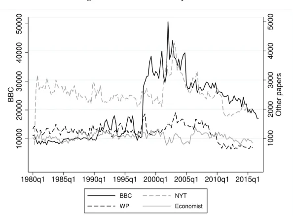
All our text data is downloaded manually from Lexis Nexis. Due to copyright issues the raw newspaper articles cannot be shared. Summarized topics and all other data and codes will be made available upon publication. The key factor in choosing our news sources is that they should be english-speaking, offer as much text as possible and long time-series. We therefore chose the New York Times (NYT), the Washington Post (WP), the Economist and the BBC Monitor (BBC). The latter source tracks broadcasts, press and social media sources in multiple languages from over 150 countries worldwide and produces translations into English.

We download an article if the name of the country or its capital appears in the title of the article. This gives us a panel of articles from all sources for over 190 countries for the period 1989Q1 to 2017Q3. In total we have access to about 700,000 articles from the New York Times, Washington Post and the Economist and 3.1 million articles from the BBC Monitor. This means that the BBC Monitor articles dominate our data. Figure 9 shows the number of articles we have for each quarter. From this is clear that the number of BBC news available from Lexis Nexis increases around 2000. Part of this increase came from a change in the headlines, which around this period often began with the country name followed by a colon and then a traditional headline. This temporary change does not affect the regional distribution substantially. In any case, the increase in the amount of news is only problematic for our forecasting exercise if the increase or decrease in the number of news somehow affects the share of news written on a specific topic. It would then become impossible to use this data effectively for forecasting as the training of the model would not produce useful forecast in the testing sample.

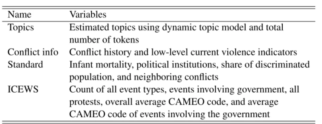
In Table 5 we summarize the different sets of predictors we use. The first model is based on our text data. This includes 5, 10, 15, 30 or 50 topic shares and the log of the word count of that quarter. The word count varies between 5 and 1226371 and is log-normally distributed with

(22)

Fig. 9: Number of Articles by Source 1000 2000 3000 4000 5000 Other papers 10000 20000 30000 40000 50000 BBC 1980q1 1985q1 1990q1 1995q1 2000q1 2005q1 2010q1 2015q1 BBC NYT WP Economist

Note: The y-axis on the left exhibits the quarterly sum of BBC articles, while the y-axis on the right exhibits the quarterly sum of articles from The Economist, New York Times, or Washington Post.

a mean of 4274 words, while the topics sum to one within each country-quarter. The second model is based on the violence data from GED. It includes dummies for the conflict history and dummies for ongoing low-level violence. The third model uses more standard variables in the literature (Goldstone et al. 2010) and includes political institutions dummies based on various dimensions of the Polity IV data, number of neighboring conflicts, the newest data on child mortality from the World Bank and the share of population which is discriminated against using data from the Geographical Research On War, Unified Platform (GROWup) (Girardin et al. 2015).

Finally, we use the ICEWS event database to generate a quarterly panel between 1995Q1 and 2016Q4. We only use events in which the source and the target of the action were in the same country. We then make a count of all 20 event types on the Conflict and Mediation Event

(23)

Table 1: Sets of Predictors

Name Variables

Topics Estimated topics using dynamic topic model and total

number of tokens

Conflict info Conflict history and low-level current violence indicators

Standard Infant mortality, political institutions, share of discriminated

population, and neighboring conflicts

ICEWS Count of all event types, events involving government, all

protests, overall average CAMEO code, and average CAMEO code of events involving the government

Observations (CAMEO) integer scale and another count of all 20 events on the CAMEO scale that involve the government either as target or as source. In addition, we generate a count of all protest events, the average CAMEO code of events involving the government, and the average CAMEO code of all events taking place in the country.

(24)

Rolling Forecast Method

In this step take the perspective of a policymaker who observes all available text and conflict until period T and has to make a forecast for period T + 1. We summarize the K topic shares

and the log of the word count in the vector, θit. We then train a forecasting model with all data

available in T using the model

y_it+1= FT(hit, θit) (1)

where yit+1 is the onset of conflict in quarter t + 1, hitis a vector of dummies capturing

post-conflict dynamics and lower levels of violence. The role of machine learning in this step is to

discipline the regularization of the model FT(hit, θit). We fix the hyperparameters in the first

sample (1989Q1-2000Q1) through cross-validation. The newest conflicts that break out in the training sample are those that break out in T . Note that this implies that, during training, we

only use data for hit and θit available until T − 1. With the resulting model we then produce

predicted out of sample values

ˆ

y_iT₊₁= FT(hiT, θiT).

which we compare to the true values yiT+1.

We then update our topic model with the news written in the next quarter, add the new information on conflicts, retrain the prediction model, and predict the probabilities of outbreaks in the following quarter. For testing, we thereby produce sequential out-of-sample forecasts,

ˆ

y_iT+1, for T + 1 = 2000Q2, 2000Q3, ..., 2017Q4. We then compare these forecasts with the

actual realizations yiT+1. In this way we get a realistic evaluation of what is possible in terms

of forecasting power in actual applications as we never use any data for testing which has been used for training purposes.

To generate FT(.) we tested predictions from k-nearest neighbor, adaptive boosting, random

forests, neural network, logit lasso regression, and ensembles of all previously mentioned mod-els. The hyperparameters are chosen by maximizing the AUC through cross-validation within

(25)

the sample before the year 2000. We found that the random forest model provides the best forecast overall. This is important as it indicates that a method with built-in safeguards against overfitting performs best in our out-of-sample test.

Why the Hard Problem is Important

Prevention is of key interest for the international community. All big international organisa-tions treat fragility and conflict risk as key problems. This is best illustrated by a joint press conference by the UN Secretary-General Antonio Guterres and the President of the World Bank Jim Yong Kim on September 21st 2017. Guterres stressed that “Preventing violent conflict is a universal concern. It is not only for those in a specific region or income bracket. We are all affected, and we must work together to end this scourge” and Kim added “While we have worked to address the impact of conflict, we need to do more early on to ensure that develop-ment programs and policies are focused on successful prevention.” The need to forecast hard cases follows directly from this need to “do more early on”. Once conflict has broken out, pre-vention has failed and so, by definition, conflict prepre-vention requires a risk evaluation for hard problem cases, i.e. cases without a recent conflict history.

Of course, it might be tempting to instead focus on cases that are easier to predict - and indeed this is what the current system of peacekeeping is geared to do. But the conflict trap does not only make prediction outside of it difficult, it is also a serious long-term threat that countries should avoid. Armed conflict has its own dynamics and a simulation of possible futures indicates that prevention in hard conflict cases has extremely high dynamic payoffs. In other words, the expected future outcome when starting from conflict and post-conflict peace are extremely similar but differ dramatically to peace in hard cases. When a country experiences an outbreak of violence in a hard-to-predict scenario its possible future changes much more dramatically. This is much less true for an outbreak of violence post-conflict.

(26)

Discussion of Estimated Topics

In this section we discuss various aspects of the estimated topics. We estimate the topic model repeatedly starting with all text until 2000Q1 and then we update every quarter using a dynamic

topic model ( ˇReh˚uˇrek and Sojka 2010). We allow the weight variational hyperparameters for

each document to be inferred by the algorithm. Before feeding the text to the machine learning algorithm we conduct standard procedures when working with text. We remove overly frequent words defined as stopwords. Then we stem and lemmatize the words before also forming two and three word combinations. Next we remove overly frequent tokens, i.e. those appearing in at least half of the articles. Finally, we also remove rare expressions appearing in less than 100 documents.

In what follows we will focus on topic models estimated in 2017Q3 as these describe all relevant text we use in our forecasting framework. Table 2 summarizes the top 10 terms in the

K = 15 topic model estimated in 2017Q3. There are three topics which are clearly related to

conflict. Topic 1, which we label the military topic, contains terms like army and military and terms indicating fighting. Topic 8, which we label the violence topic, has terms like province and other location indicators mixed with words indicating fighting.

In Figure 10 we show the timeline for these two topics in our sample period for Afghanistan, Angola, Iraq and Ukraine. The aim is to show that the two topics give a fairly good idea of the different conflict histories in the respective countries. In the image for Afghanistan we see that both topic shares fluctuate wildly and are very high throughout the period, accounting for between 6 and 21 percent of all news written on Afghanistan. Most recently, more is written on violence. In Angola writing on conflict topics decreases dramatically following the cease-fire in 2002. In Iraq the invasion of 2003 is very clearly visible. In Ukraine the start of the turmoil in 2014 and outright war later is clearly visible in the news text. Of course, such movements in conflict topics are only helpful for forecasting if they anticipate conflict. In Figure 21 we show this for the military topic.

(27)

Table 2: Top Ten Keywords of 15 Topic Model Using All Text Until 2017Q3

Nr Label Keywords

0 Justice court, case, law, investig, right, human, arrest, offic, human_right, polic

1 Military* forc, militari, armi, oper, border, arm, group, region, secur, troop

2 Media ministri, medium, channel, region, inform, servic, say, head, accord, author

3 Daily life websit, user, school, bit, com, child, time, onlin, woman, work

4 Terror* islam, terror, terrorist, arab, muslim, group, leader, sharif, say, persian

5 Intl relations secur, intern, region, relat, cooper, issu, develop, support, import, council

6 Politics trump, time, polit, war, say, bit, polici, make, want, like

7 Investment project, compani, trade, develop, oil, energi, gas, product, construct, industri

8 Violence* attack, polic, kill, video, provinc, citi, secur, district, area, local

9 Diplomacy beij, cooper, visit, tie, myanmar, bilater, develop, headlin, relat, trade

10 Economics cent, bank, websit, compani, econom, economi, dollar, billion, busi, financi

11 State visits meet, talk, agreement, visit, issu, prime, peac, negoti, discuss, offici

12 Cold war* nuclear, missil, websit, defenc, ukrainian, militari, test, korean, dprk, weapon

13 Elections parti, elect, opposit, polit, vote, parliament, ial, leader, constitut, candid

14 Asia sea, korean, sanction, offici, abe, washington, secur, donald, island, militari

Note: The labels are arbitrary and have no influence on the prediction model. The topics marked by ‘*’ are considered violence topics.

(28)

Fig. 10: Military and Violence Topic Shares Across Time and Countries 0 .05 .1 .15 .2 .25 1990q1 1995q1 2000q1 2005q1 2010q1 2015q1 Afghanistan 0 .05 .1 .15 .2 .25 1990q1 1995q1 2000q1 2005q1 2010q1 2015q1 Angola 0 .05 .1 .15 .2 .25 1990q1 1995q1 2000q1 2005q1 2010q1 2015q1 Iraq 0 .05 .1 .15 .2 .25 1990q1 1995q1 2000q1 2005q1 2010q1 2015q1 Ukraine Military Violence

(29)

Table 3: Models

Technique Brief description

Logit Linear estimation of log-odds

K-nearest neighbor Classifies a vector according to similarity

Neural network Artificial neurons split into layers including feedback effects

AdaBoost Weighted sum of other learning algorithm (‘weak learner’)

Random forest Average over many decision trees

Stacking Ensemble using logit based on five predictions

Prediction Algorithms

To explore the gains from supervised learning we look at five different algorithms specified in Table 3 which are trained with the available data using a Python implementation (Pedregosa et al. 2011). We standardize the data in order to improve the performance of machine learning algorithms such as neural networks.

The five individual supervised prediction algorithms we use are a logistic lasso regression, k-nearest neighbor (kNN), neural network, AddaBoost, and random forest. Providing very brief summaries, the logit lasso estimates the log odds of an event using a linear expression while choosing which variables to include through a penalizing term. kNN is a non-parametric method used for classification in which the algorithm classifies a vector according to similarity. If a vector of predictors looks similar to those with many onsets, then it is more likely to classify a given set of predictors as an onset. Neural networks are a complex web of artificial neurons split into layers which are meant to resemble the functioning of neurons in a brain. Thereby, the technique can capture non-linearities through feedback effects between the multiple layers and because neurons might not fire until reaching a threshold. AdaBoost, which is short for Adaptive Boosting, uses output of other learning algorithms, referred to as ‘weak learners’, aggregated as a weighted sum. In our case, the weak learner is chosen to be a decision tree of depth one. AdaBoost is adaptive in the sense that weak learners are tweaked in favor of instances misclassified by previous classifiers.

(30)

Random forests construct many decision trees at training time and then averages across the predictions of the entire collection of trees, i.e. the forest. This way of modeling risk has the particular appeal that important features like conflict history will be chosen early if available, and the model therefore adapts automatically to the hard problem. We discuss this feature in the main text.

While the final evaluation of our model is carried out strictly out-of-sample, i.e. in the future without using any contemporaneous or future information, the training of the models is per-formed through cross-validation. More specifically, the method used is k-fold cross-validation, where the training set is split into k smaller sets. For each of the k ‘folds’ the following pro-cedure is performed: A model is trained using k − 1 of the folds as training data; using the remaining data a test is carried out by computing our chosen performance measure, the AUC. The performance measure reported by k-fold cross-validation is then the average of the values computed in the loop. Each individual algorithm also requires the specification of hyperparam-eters by the user. For each set of predictors, we choose these hyperparamhyperparam-eters by doing a grid search using the sample until the year 2000 and then selecting the hyperparameters that gener-ate the highest AUC. Note, that this will understgener-ate the performance of the forecasting model slightly if more information leads to a deeper or modified model in later years.

In Table 4 we present the chosen hyperparameters for the random forest. We see that with text alone, random forests tend to be deeper than when adding conflict history and information about current violence.

Additional Results

In the following section we show additional results, including for a greater cut-off of 500 battle deaths. In Figure 11 we see that for the very large cutoff in terms of battle deaths, the onset of conflict becomes relatively easy to predict. The harder it is to predict conflict, the more topics add to the forecasting power. In particular, when forecasting the hard cases of any violence,

(31)

Table 4: Hyperparameters

Predictors Random forest

Depth Trees

Any violence

Text 7 400

Conflict info 4 10

Text & conflict info 7 500

Armed conflict

Text 5 250

Conflict info 4 50

Civil war

Text 5 100

Conflict info 1 150

Note: Hyperparameters chosen through cross-validation within the sample before year 2000.

the text-only model provides a relatively good forecast given the difficulty of predicting these events. When predicting civil war, the presence of any violence or armed conflict are powerful predictors, even in the hard cases, which is why it is difficult to augment the prediction of further escalation even with text. However, one should note that text alone also achieves high levels of accuracy for all and the hard cases.

In Figure 12 we show separation plots for each of the outcomes for predictions using topics and conflict information. The figures order predictions by their rank on the x-axis and plot the predicted level of risk using the red dashed line on the y-axis. The black vertical lines indicate actual onsets. For all outcomes, onsets tend to be bunched on the right side of the panel where the predicted probabilities are highest. But separation plots have the additional advantage of providing an idea of where the model fails to predict conflict. The 5000 lowest risk observations contain only 19 onsets without clear common features.

In Figure 13 we show the AUC for ROC curves computed for every single year for each of the three outcomes. We see that the AUCs stay constant or seem to increase slightly over time

(32)

Fig. 11: ROC Curves of Forecasting Civil War

0.0 0.2 0.4 0.6 0.8 1.0

False Positive Rate

0.0 0.2 0.4 0.6 0.8 1.0 Tru e Po si tive R at e All cases Text (area = 0.92) Conflict info (area = 0.96) Text & conflict info (area = 0.97)

0.0 0.2 0.4 0.6 0.8 1.0

False Positive Rate

0.0 0.2 0.4 0.6 0.8 1.0 Hard cases Text (area = 0.94) Conflict info (area = 0.94) Text & conflict info (area = 0.97)

Note: The random forest has a tree depth of 2 and 125 trees. ‘Text’ contains 15 topics and token counts and ‘conflict info’ contains 4 dummies capturing time passed since the last conflict and a dummy each for the presence of any violence and armed conflict. Hard cases are defined as not having had civil war in 10 years.

especially when using text only. We attribute this positive trend to the increase in the training sample over time.

A problem in Figure 13 is that we have only relatively few onsets, which means that the general trend in model performance is hard to evaluate due to high volatility. In Figure 14 we therefore show the results of a cross-validation exercise in which we fix the number of trees in the forest but run a gridsearch over the optimal tree depth and record the maximal AUC of this cross validation. The results again suggest a clear upward trend in the cross-validated AUC which is in line with the out-of-sample AUC in Figure 13. Interestingly, the cross validation AUC is significantly below the true out-of-sample AUC. This is most likely because the folds in the cross validation do not take the panel structure into account and train models on very different parts of the data. Our out-of-sample always uses the most recent past data to predict one quarter or year ahead which is less challenging. The optimal tree depth fluctuates from quarter to quarter but there are no broader trends in the optimal depth.

(33)

fore-Fig. 12: Separation Plot of Forecasting Violence using Text and Conflict Information 0 2000 4000 6000 8000 10000 12000 Rank of prediction 0.0 0.2 0.4 0.6 0.8 1.0 Pre dict ed risk Any violence 0 2000 4000 6000 8000 10000 12000 Rank of prediction 0.0 0.2 0.4 0.6 0.8 1.0 Armed conflict

Predicted risk Onsets

0 2000 4000 6000 8000 10000 12000 Rank of prediction 0.0 0.2 0.4 0.6 0.8 1.0 Civil war

Note: ‘Text’ contains 15 topics and token counts and ‘conflict info’ contains 4 dummies capturing time passed since the last conflict and dummies for the presence of lower levels of violence.

casting model can be developed as changes in the international context prevent generalization. In both figures forecast performance with text tends to improve with increasing sample size de-spite a dramatically changing international context and a completely new set of violence onsets.

(34)

Fig. 13: AUC by Year of Forecasting Violence 2000 2005 2010 2015

Year

0.65 0.70 0.75 0.80 0.85 0.90 0.95 1.00

AU

C

Any violence 2000 2005 2010 2015

Year

Armed conflict

Text

Conflict history dummies

Text & conflict history dummies

2000 2005 2010 2015

Year

Civil war

(35)

Fig. 14: Cross Validated AUC Over Time .87 .875 .88 .885 AUC 2 4 6 8 Depth 2000q1 2004q3 2009q1 2013q3 2018q1 Cross−validation sample Any violence, 500 trees

.905 .91 .915 .92 AUC 2 3 4 5 6 Depth 2000q1 2004q3 2009q1 2013q3 2018q1 Cross−validation sample Armed conflict, 425 trees

AUC in cross validation Optimal tree depth

Note: Figures show the cross validated AUC as a black solid line and the optimal tree depth as a dashed line. The cross validation sample always runs from 1989Q1 to the time given on the x-axis.

(36)

Table 5: Sets of Predictors

Name Variables

Topics Estimated topics using dynamic topic model and total

number of tokens

Conflict info Conflict history and low-level current violence indicators

Standard Infant mortality, political institutions, share of discriminated

population, and neighboring conflicts

ICEWS Count of all event types, events involving government, all

protests, overall average CAMEO code, and average CAMEO code of events involving the government

In Figure 15 we compare the performance of the topics to standard variables related to pol-itics and economics traditionally used in the literature. Variables such as infant mortality are available for less countries and years. For the sake of comparability, we only use overlapping predictions for evaluation, i.e. country-quarters in which the availability of data allow predic-tions for both sets of variables. The panels on the top depict the ROC curves for all cases while on the bottom we present the curves for the hard cases only. The left panels refer to any violence, the middle to armed conflict, and the right to civil war.

We find that text, in particular for previously peaceful countries, provides superior informa-tion for predicinforma-tion. Moreover, topics have the advantage that they are based on newspaper text which is available on a daily basis. Standard variables, on the other hand, are available with lags up to several years, which we do not consider in this comparison. Therefore, the presented predictive power of these variables can be considered an upper bound.

In Figure 16 we compare the performance of the topics to events from the Integrated Conflict Early Warning System (ICEWS) database. The ICEWS model we build relies on over 40 event counts. We use 20 counts of all CAMEO event categories that have their target on the territory of the country. We also take the 20 counts involving the government. In addition, we add the average CAMEO scale number of all events. Here, again, we find that topics combined with conflict history dummies perform at least as good the event data combined with conflict history dummies for all cutoffs evaluated. Adding events to topics with conflict info only provides

(37)

Fig. 15: AUC Curves of Forecasting Violence Using Text Compared to Standard Variables 0.0 0.2 0.4 0.6 0.8 1.0 0.0 0.2 0.4 0.6 0.8 1.0 Tru e Po si tive R at e

Text (area = 0.75) Text & conflict info (area = 0.87) Standard & conflict info (area = 0.85) Text & Standard & conflict info (area = 0.86)

0.0 0.2 0.4 0.6 0.8 1.0 0.0 0.2 0.4 0.6 0.8 1.0

Civil war (all cases)

0.0 0.2 0.4 0.6 0.8 1.0

Civil war (hard cases)

Note: ‘Text’ contains 15 topics and token counts, ‘conflict info’ contains 4 dummies capturing time passed since the last conflict and dummies for the presence of lower levels of violence, and ‘standard’ contains Infant mortality, political institutions, share of discriminated population, and neighboring conflicts. Hard cases are

defined as not having had conflict in 10 years.

an improvement when forecasting armed conflict. This is interesting because it suggests that ICEWS events provide a good way to capture a situation which might escalate but that the risk of any violence onset is too diffuse to be identified with supervised learning. The unsupervised learning approach we choose instead is more useful here.

We show the performance of each of these individual prediction models using text only (Figure 17) and both text and conflict information (Figure 18). Across all outcomes it seems that the random forest is the algorithm performing best. But it stands out particularly when

(38)

Fig. 16: AUC Curves of Forecasting Violence Using Text Compared to ICEWS 0.0 0.2 0.4 0.6 0.8 1.0 0.0 0.2 0.4 0.6 0.8 1.0 Tru e Po si tive R at e

Text (area = 0.78)

Text & conflict info (area = 0.88)

ICEWS & conflict info (area = 0.86) Text & ICEWS & conflict info (area = 0.87)

0.0 0.2 0.4 0.6 0.8 1.0 0.0 0.2 0.4 0.6 0.8 1.0

Text (area = 0.86) Text & conflict info (area = 0.92) ICEWS & conflict info (area = 0.91) Text & ICEWS & conflict info (area = 0.93)

0.0 0.2 0.4 0.6 0.8 1.0 0.0 0.2 0.4 0.6 0.8 1.0

0.0 0.2 0.4 0.6 0.8 1.0

Note: ‘Text’ contains 15 topics and token counts, ‘conflict info’ contains 4 dummies capturing time passed since the last conflict and dummies for the presence of lower levels of violence, and ‘ICEWS’ contains a count of all event types, events involving government, all protests, overall average CAMEO code, and average CAMEO code

of events involving the government. Hard cases are defined as not having had conflict in 10 years.

predicting any violence with conflict history and text. Here the random forest reaches an AUC of 0.83 whereas the logit lasso only reaches and AUC of 0.68. This is consistent with the idea that the random forest receives an advantage because the model is able to use the information contained in the text conditional on conflict history. This is less important when predicting armed conflict as violence escalation is much more important there.

In Figure 19 we show that the models performance is not specific to 15 topics. The model performs similarly for 5, 10 and 30 topics. For 50 topics, however, the performance starts to

(39)

Fig. 17: ROC Curves of Forecasting Violence with Individual Prediction Models Using Only Text 0.0 0.2 0.4 0.6 0.8 1.0 0.0 0.2 0.4 0.6 0.8 1.0 Tru e Po si tive R at e Any violence Neighbor (area = 0.76) Logit (area = 0.76) Neural (area = 0.76) AdaBoost (area = 0.76) RandomForest (area = 0.78) 0.0 0.2 0.4 0.6 0.8 1.0 0.0 0.2 0.4 0.6 0.8 1.0 Armed conflict Neighbor (area = 0.84) Logit (area = 0.85) Neural (area = 0.85) AdaBoost (area = 0.82) RandomForest (area = 0.86) 0.0 0.2 0.4 0.6 0.8 1.0 0.0 0.2 0.4 0.6 0.8 1.0 Civil war Neighbor (area = 0.89) Logit (area = 0.91) Neural (area = 0.92) AdaBoost (area = 0.90) RandomForest (area = 0.92) 0.0 0.2 0.4 0.6 0.8 1.0

False Positive Rate 0.0 0.2 0.4 0.6 0.8 1.0 Tru e Po sit ive R ate Previously peaceful Neighbor (area = 0.82) Logit (area = 0.83) Neural (area = 0.83) AdaBoost (area = 0.83) RandomForest (area = 0.84) 0.0 0.2 0.4 0.6 0.8 1.0

False Positive Rate 0.0 0.2 0.4 0.6 0.8 1.0 Previously peaceful Neighbor (area = 0.69) Logit (area = 0.81) Neural (area = 0.81) AdaBoost (area = 0.73) RandomForest (area = 0.76) 0.0 0.2 0.4 0.6 0.8 1.0

False Positive Rate 0.0 0.2 0.4 0.6 0.8 1.0 Previously peaceful Neighbor (area = 0.88) Logit (area = 0.91) Neural (area = 0.92) AdaBoost (area = 0.96) RandomForest (area = 0.94)

Note: ‘Text’ contains 15 topics and token counts. Hard cases are defined as not having had conflict in 10 years.

become worse, in particular concerning the hard problem, due to overfitting.

Given our unbalanced sample due to the low frequency of violence, we experiment with upsampling using a Python package (Lemaître, Nogueira and Aridas 2017). We find that in-sample performance is boosted but out-of-in-sample performance is subpar as can be seen in Figure 20, especially when the number of predictors grows. The algorithm tailors predictions to certain events, which then do not generalize, a classical case of overfitting. We observe similar patterns when including continent or region fixed effects without upsampling.

(40)

Fig. 18: ROC Curves of Forecasting Violence with Individual Prediction Models Using Text and Conflict Information

0.0 0.2 0.4 0.6 0.8 1.0 0.0 0.2 0.4 0.6 0.8 1.0 Tru e Po si tive R at e Any violence Neighbor (area = 0.90) Logit (area = 0.90) Neural (area = 0.90) AdaBoost (area = 0.89) RandomForest (area = 0.89) 0.0 0.2 0.4 0.6 0.8 1.0 0.0 0.2 0.4 0.6 0.8 1.0 Armed conflict Neighbor (area = 0.91) Logit (area = 0.92) Neural (area = 0.92) AdaBoost (area = 0.91) RandomForest (area = 0.93) 0.0 0.2 0.4 0.6 0.8 1.0 0.0 0.2 0.4 0.6 0.8 1.0 Civil war Neighbor (area = 0.96) Logit (area = 0.96) Neural (area = 0.96) AdaBoost (area = 0.94) RandomForest (area = 0.97) 0.0 0.2 0.4 0.6 0.8 1.0

False Positive Rate 0.0 0.2 0.4 0.6 0.8 1.0 Tru e Po sit ive R ate Previously peaceful Neighbor (area = 0.73) Logit (area = 0.68) Neural (area = 0.68) AdaBoost (area = 0.75) RandomForest (area = 0.83) 0.0 0.2 0.4 0.6 0.8 1.0

False Positive Rate 0.0 0.2 0.4 0.6 0.8 1.0 Previously peaceful Neighbor (area = 0.69) Logit (area = 0.83) Neural (area = 0.83) AdaBoost (area = 0.75) RandomForest (area = 0.84) 0.0 0.2 0.4 0.6 0.8 1.0

False Positive Rate 0.0 0.2 0.4 0.6 0.8 1.0 Previously peaceful Neighbor (area = 0.93) Logit (area = 0.96) Neural (area = 0.96) AdaBoost (area = 0.93) RandomForest (area = 0.97)

very good predictors of the outbreak of violence. Nonetheless, text summarized by topics adds useful information to predict topics, in particular in countries without current violence or a conflict history.

(41)

Fig. 19: AUC Curves of Forecasting Violence with Random Forest Using Text while Varying Number of Topics 0.0 0.2 0.4 0.6 0.8 1.0 0.0 0.2 0.4 0.6 0.8 1.0 Tru e Po siti ve Ra te

5 Topics (area = 0.72) 10 Topics (area = 0.77) 15 Topics (area = 0.78) 30 Topics (area = 0.79) 50 Topics (area = 0.80) 0.0 0.2 0.4 0.6 0.8 1.0 0.0 0.2 0.4 0.6 0.8 1.0

5 Topics (area = 0.82) 10 Topics (area = 0.86) 15 Topics (area = 0.86) 30 Topics (area = 0.86) 50 Topics (area = 0.86) 0.0 0.2 0.4 0.6 0.8 1.0 0.0 0.2 0.4 0.6 0.8 1.0

5 Topics (area = 0.86) 10 Topics (area = 0.88) 15 Topics (area = 0.92) 30 Topics (area = 0.89) 50 Topics (area = 0.89) 0.0 0.2 0.4 0.6 0.8 1.0

False Positive Rate

0.0 0.2 0.4 0.6 0.8 1.0 Tru e Po sit ive Ra te

False Positive Rate

0.0 0.2 0.4 0.6 0.8 1.0

False Positive Rate

0.0 0.2 0.4 0.6 0.8 1.0

5 Topics (area = 0.87) 10 Topics (area = 0.86) 15 Topics (area = 0.94) 30 Topics (area = 0.89) 50 Topics (area = 0.89)

Note: Predictors include specified number of topics and token counts as well as dummies for time passed since the last conflict and dummies for the presence of lower levels of violence. Hard cases are defined as not having

had conflict in 10 years.

Additional Material on How Onset is Predicted

Dynamic Predicted Risk and Case Studies

As we show in the main text that there are several strong positive and negative associations be-tween different topics and conflict onset. Importantly, these relationships are not only varying between countries but also within countries over time so that meaningful dynamic risk profiles result from our forecasts. To illustrate the dynamic properties of two topics, Figure 21 shows the movement of the economics (left) and military (right) topic shares and the 95 percent con-fidence interval before the onset of armed conflict in the full sample. The figure is based on