HAL Id: hal-00665660
https://hal.archives-ouvertes.fr/hal-00665660
Submitted on 25 Jun 2019HAL is a multi-disciplinary open access archive for the deposit and dissemination of sci-entific research documents, whether they are pub-lished or not. The documents may come from teaching and research institutions in France or abroad, or from public or private research centers.
L’archive ouverte pluridisciplinaire HAL, est destinée au dépôt et à la diffusion de documents scientifiques de niveau recherche, publiés ou non, émanant des établissements d’enseignement et de recherche français ou étrangers, des laboratoires publics ou privés.
Global Identification of Robot Drive Gains Parameters
Using a Known Payload and Weighted Total Least
Square Techniques
Maxime Gautier, Sébastien Briot
To cite this version:
Maxime Gautier, Sébastien Briot. Global Identification of Robot Drive Gains Parameters Using a Known Payload and Weighted Total Least Square Techniques. 16th IFAC Symposium on System Identification (SYSID 2012), Jul 2012, Bruxelles, Belgium. �hal-00665660�
and Weighted Total Least Square Techniques
Maxime Gautiera,b and Sébastien Briota
a Institut de Recherche en Communications et Cybernétique de Nantes (IRCCyN) 44321 Nantes France
(Tel: +33240376960; e-mail: {Maxime.Gautier, Sebastien.Briot}@irccyn.ec-nantes.fr).
b University of Nantes 44321 Nantes France
Abstract: Off-line robot dynamic identification methods are based on the use of the Inverse Dynamic Identification Model (IDIM), which calculates the joint forces/torques that are linear in relation to the dynamic parameters, and on the use of linear least squares technique to calculate the parameters (IDIM-LS technique). The joint forces/torques are calculated as the product of the known control signal (the current reference) by the joint drive gains. Then it is essential to get accurate values of joint drive gains to get accurate identification of inertial parameters. In the previous works, it was proposed to identify each gain separately. This does not allow taking into account the dynamic coupling between the robot axes. In this paper the global joint drive gains parameters of all joints are calculated simultaneously. The method is based on the weighted total least squares solution of an over-determined linear system obtained with the inverse dynamic model calculated with available current reference and position sampled data while the robot is tracking one reference trajectory without load on the robot and one trajectory with a known payload fixed on the robot. The method is experimentally validated on an industrial 6 joint Stäubli TX-40 robot.
1. INTRODUCTION
Several schemes have been proposed in the literature to identify the dynamic parameters of robots (Gautier and Khalil 1990), (Hollerbach et al. 2008), (Khalil and Dombre 2002), (Khosla and Kanade 1985), (Lu et al. 1993). Most of the dynamic identification methods have the following features: - the use of an Inverse Dynamic Identification Model
(IDIM) which calculates the joint force/torque linear in relation to the dynamic parameters,
- the construction of an over-determined linear system of equations obtained by sampling IDIM while the robot is tracking some trajectories in closed-loop control,
- the estimation of the parameter values using least squares techniques (LS). This procedure is called the IDIM-LS technique.
The experimental works have been carried out either on prototypes in laboratories or on industrial robots and have shown the benefits in terms of accuracy in many cases. Good results can be obtained provided two main conditions are satisfied:
- a well-tuned derivative band-pass filtering of joint position is used to calculate the joint velocities and accelerations,
- the accurate values of joint drive gains g are known to
calculate the joint force/torque as the product of the known control signal calculated by the numerical controller of the robot (the current references) by the joint drive gains (Restrepo and Gautier 1995).
This needs to calibrate the drive train constituted by a current
controlled voltage source amplifier with gain Gi which
supplies a permanent magnet DC or a brushless motor with
torque constant Kt coupled to the link through direct or gear
train with gear ratio N. Because of large values of the gear
ratio for industrial robots, (N>50), joint drive gain,
i t
g NG K , is very sensitive to errors in Giand Kt which
must be accurately measured from special, time consuming , heavy tests, on the drive chain (Restrepo and Gautier 1995), (Corke 1996).
Several papers on the topic of the joint drive gains identification have been published in the past (Corke 1996), (Gautier and Briot 2011a,b), (Restrepo and Gautier 1995), but all of them propose to identify each joint gain separately. This does not allow taking into account the dynamic coupling between the robot joint force/torque.
In this paper it is proposed a new method for the global identification of the joint drive gains, using current reference and position sampled data measured while the robot is tracking one reference trajectory without load fixed on the robot and one trajectory with a known payload fixed on the robot. Contrary to the previous works, all drive gains are calculated in one step by the weighted total LS solution (WTLS) of an over-determined system in order to take into account the coupling between the robot axes. The method is experimentally validated on a 6 joint industrial Stäubli TX-40 robot.
2. USUAL DYNAMIC IDENTIFICATION METHOD
2.1 Inverse Dynamic Identification Model (IDIM)
be linearly written in term of a
n1
vector of standardparameters (Hollerbach et al. 2008), (Khalil and Dombre st
2002). The modified Denavit and Hartenberg notation allows obtaining a dynamic model that is linear in relation to a set of
standard dynamic parameters, χst:
( ) ( )
idm q,q,q, st st q,q,q st
(1)
where: idm
is the
n1
vector of the input efforts st is the
n n st
jacobian matrix of τidm, with respect tothe
nst1
vector χst of the standard parameters givenby 1T 2T ... n T T
st st st st
q,q,q are the vectors of the joint positions, velocities and accelerations, respectively.
For rigid robots, there are 14 standard parameters by link and joint. For the joint and link j, these parameters can be
regrouped into the (14×1) vector j
st
(Khalil and Dombre 2002): j j T st XX XY XZ YY YZ ZZ MX MY MZ M Ia Fv Fcj j j j j j j j j j j j j off (2) where: j j j j j j
XX , XY , XZ , YY , YZ , ZZ are the 6 components of the inertia matrix of link j at the origin of frame j .
j j j
MX , MY , MZ are the 3 components of the first moment
of link j , Mj is the mass of link j , Iaj is a total inertia moment for rotor and gears of actuator j .
j
Fv , Fcj are the visquous and Coulomb friction coefficients
of the transmission chain, respectively,
j j j
off offFS off
is an offset parameter which regroups the
amplifier offset offjand the asymmetrical Coulomb friction
coefficient offFSj.
The identifiable parameters are the base parameters which are the minimum number of dynamic parameters from which the dynamic model can be calculated. They are obtained from the standard inertial parameters by regrouping some of them by means of linear relations (Mayeda et al. 1990), which can be determined for the serial robots using simple closed-form rules (Gautier and Khalil 1990), (Khalil and Dombre 2002), or by numerical method based on the QR decomposition (Gautier 1991).
The minimal dynamic model can be written using the nb
base dynamic parameters as follows:
( )
idm q,q,q
(3)
where is obtained from by eliminating the columns st
corresponding to the non identifiable parameters.
Because of perturbations due to noise measurement and
modelling errors, the actual force/torque differs from τidm
by an error, e , such that:
( ) idm τ e q,q,q e (4) where 1 0 0 1 0 0 0 0 n n v g v g v g (5)
v is the (n n ) matrix of the actual current references of the current amplifiers (vj
corresponds to actuator j) and g
is the (n1) vector of the joint drive gains (gj
corresponds
to actuator j). Equation (4) represents the IDIM.
2.2 Least Squares Identification of the Dynamic Parameters (IDIM-LS)
The off-line identification of the base dynamic parameters
is considered, given measured or estimated off-line data for τ and
q, q, q , collected while the robot is tracking some
planned trajectories. The model (4) is sampled and low pass filtered in order to get an over-determined linear system of(n r ) equations and nb unknowns:
ˆ ˆ ˆ
Y τ W q,q,q χ ρ (6)
where
( )ˆq, q, q are an estimation of ˆ ˆ ( )q, q, q , obtained by band-pass filtering and sampling the measure of q (Gautier 1997),
ρ is the (r1) vector of errors,
ˆ ˆ ˆ
W q, q, q is the (r n b) observation matrix.
Using the base parameters and tracking “exciting” reference trajectories, a well conditioned matrix W is obtained. The LS solution ˆχ of (6) is given by:
T 1 T
ˆχ W W W Y W Y (7)
It is computed using the QR factorization of W .
Standard deviations , are estimated assuming that ˆi W is a
deterministic matrix and , is a zero-mean additive
independent Gaussian noise, with a covariance matrix C,
such that:
T 2
( ) r
C E ρρ I (8)
E is the expectation operator and Ir, the (r r ) identity
matrix. An unbiased estimation of the standard deviation
is:
2
2 ˆ ( )
ˆ Y -W r b
(9)
The covariance matrix of the estimation error is given by:
T 2 T 1 [( )( ) ] ( ) ˆ ˆ ˆ ˆ ˆ C E χ χ χ χ W W . ( ) i 2 ˆ Cˆ ˆ i,i
is the ith diagonal coefficient of
ˆ ˆ
C (10)
100
ri i
ˆ ˆ ˆi
% , for ≠ 0 ˆi (11)
The ordinary LS can be improved by taking into account
different standard deviations on joint j equations errors
(Gautier 1997). Data in Y and W of (6) are sorted and
weighted with the inverse of the standard deviation of the error calculated from OLS solution of the equations of joint
j (Gautier 1997).
This weighting operation normalises the errors in (6) and gives the weighted LS estimation of the parameters (IDIM-WLS).
3. GLOBAL IDENTIFICATION OF THE JOINT DRIVE GAINS
3.1 IDIM Including a Payload and Drive Gains
The payload is considered as a link n1 fixed to the link n
of the robot. Only nkL of its parameters are considered
known. The model (4) becomes:
T T T T uL kL uL kL v g e (12) where: kL
is the (nkL1) vector of inertial parameters of the
payload which are estimated with a CAD software or measured with a balance,
uL
is the ((10nkL) 1) vector of the unknown inertial
parameters of the payload, kL
is the (n n kL) jacobian matrix of , with respect to idm the vector , kL
uL
is the (n(10nkL)) jacobian matrix of , with idm
respect to the vector . uL
3.2 Weighted Total Least Squares Identification of the Drive Gains (IDIM-WTLS)
Details on the Total LS (TLS) identification method can be found in (Van Huffel and Vandewalle 1991) and many papers of the same authors. This method has been applied in (Gautier et al. 1994) for the identification of the drive gains and the dynamic parameters on a two degrees of freedom robot (dof) but gives arguable results due to the lack of an accurate scale factor. In this paper three major improvements are proposed:
- the accurate scaling of parameters using the precise
weighed value of an additional payload mass;
- a weighting procedure of rows and columns of the
observation matrix taking into account an a priori confidence on the measures.
- an experimental validation on a 6 dof industrial robot
which shows the efficiency of these approaches.
In order to identify the payload parameters, it is necessary that the robot carried out two trajectories: (a) without the payload and (b) with the payload fixed to the end-effector
(Khalil et al. 2007). The sampling and filtering of the model IDIM (12) can be then written as:
0 T a a T T T uL kL b b uL kL V W 0 Y g V W W W (13) where: a
V is the matrix of v samples in the unloaded case, b
V is the matrix of v samples in the loaded case,
1 1 2 2 0 0 0 0 0 0 j i , i j i , j i i i j n i ,r / n i v V v V V , V v V , with i =a, b (14) j i,k
v is the k-th sample of current reference for actuator j,
a
W is the observation matrix of the robot in the unloaded
case, b
W is the observation matrix of the robot in the loaded case,
uL
W is the observation matrix of the robot corresponding to
the unknown payload inertial parameters, kL
W is the observation matrix of the robot corresponding to
the known payload inertial parameters. Eq. (13) becomes: tot tot W , (15) where 0 0 a a tot b b uL kL kL W V W W V W W is a r( + +11n nb nkL) matrix, and T T T T tot g uL is a ( + +11n nb nkL) vector
and is a scalar which should be equal to 1.
Without perturbation, 0 and Wtotshould be rank deficient
to get the solutions tot 0 depending on a scale
coefficient . However because of the measurement
perturbations, Wtot is a full rank matrix. Therefore, the
system (15) is replaced by the compatible system closest to (15) with respect to the Frobenius norm:
0
tot tot
ˆ ˆ
W , (16)
where Wˆtot is the rank deficient matrix, with the same
dimension as Wtot, which minimizes the Frobenius norm
tot ˆtot F W W , T T T T tot uL ˆ ˆ ˆ ˆg ˆ
is the solution of the compatible system closest to (15).
tot ˆ
W can be computed thanks to the Singular Value
Decomposition (SVD) of Wtot (Golub and Van Loan 1996):
i T tot diag( s ) W U V 0 , (17)
where U and V are (r r and ) ( + +11n nb nkL) ( + +11n nb nkL) orthonormal matrices, respectively, and
i
diag( s ) is a (( + +11n nb nkL) ( + +11 n nb nkL)) diagonal
matrix with singular values si of Wtot sorted in decreasing
order. The solution of (16) is given by:
11 11 11 b kL b kL b kL T tot tot n n n n n n n n n ˆ W W s U V , (18)
where sn n b 11nkL is the smallest singular value of Wtot and
11
b kL
n n n
U (Vn n b 11nkL, resp.) the column of U (V, resp.)
corresponding to sn n b 11nkL. Then, the normalized optimal
solution n tot ˆ ( n 1 tot ˆ
) is given by the last column of V,
11 b kL n tot n n n ˆ V (Gautier et al. 1994).
There are infinity of vectors n
tot tot
ˆ ˆ
that can be obtained
by a scale factor . A unique solution * n
tot ˆ tot
ˆ ˆ
can be
found by taking into account that the last value of *
tot ˆ
should be equal to 1, i.e. ˆ 1/ˆ.
In order to improve the estimation of *
tot
ˆ
, the rows and
columns of Wtot are weighted taking into account the
confidence on the measures. Two types of weighting factors are used:
1. As proposed in IDIM-WLS (Gautier 1997) (section 2.2), to improve the ordinary LS, each row corresponding to joint j equation is weighted by the inverse of ˆj
;
2. It is also proposed to weight the columns of the observation matrix in order to take into account the a
priori relative confidence between the columns. Indeed,
as explained in section 2.2, the coefficients of matrices a
W , Wb, WuL and WkL are calculated with the values of
( )ˆq, q, q estimatedˆ ˆ by band-pass filtering and sampling the measure of q. Therefore, the coefficients of these
columns are considered less accurate than Va and Vb
obtained with the direct measures of v. In order to
increase the confidence on these columns, Va and Vb
are weighted by a factor and the new system becomes:
w w tot tot W (19) where 0 0 a a w tot b b uL kL kL W V W W V W W , and w T T T T tot g / uL .
3.3 Discussion on the A Priori Knowledge of the Payload Parameters and on the Choice of the Weighting Factors
The accuracy of ˆ depends on the accuracy of , kL
depending on the knowledge of the payload parameters.
The most accurate payload parameter is the mass value ML
that can be accurately measured using a weighing machine.
The choice of ˆj
to weight the rows of p
tot
W is physically
meaningful but the choice of parameter is not straightforward. In the remainder, it is proposed to minimize
the relative norm of error ( ) Y( ) W ˆ( ) with
respect to . The value ˆ 5 gives the best results which are presented in the following section.
4. CASE STUDY
4.1 Description of the TX-40 Kinematics
The Stäubli TX-40 robot (Fig. 1) has a serial structure with six rotational joints. Its kinematics is defined using the modified Denavit and Hartenberg notation (MDH) (Khalil and Dombre 2002). In this notation, the link j fixed frame is defined such that the zj axis is taken along joint j axis and
the xj axis is along the common normal between zj and
j 1
z (Fig. 1). The geometric parameters defining the robot
frames are given in Table 1. The payload is denoted as the
link 7. The parameter , means that joint j is j 0
rotational, j and dj parameterize the angle and distance
between zj 1 and zj along xj 1 , respectively, whereas j and rj parameterize the angle and distance between xj 1 and
j
x along zj, respectively. For link 7, j 2 means that the link 7 is fixed on the link 6. Since all the joints are rotational
then is the joint position value qj j given by the CS8C
controller of the TX-40 robot, except for joints 2 and 3 where the MDH notation differs the Staübli variables (Table 1):
5 z 4,5,6 x x x 4 rl 4,6 z z 3 z 3 x 3 d 2 z 3 rl 0,1 z z 0, ,1 2 x x x
Fig. 1. Link frames of the TX-40 robot Table 1.
Geometric parameters of the TX-40 robot with the payload
j j j dj j rj 1 0 0 0 q1 0 2 0 0 q2 0 3 0 0 d3 = 0.225 m q3 rl3 = 0.035 m 4 0 0 q4 rl4 = 0.225 m 5 0 0 q5 0 6 0 0 q6 0 7 2 0 0 0 0
2
2 q2 /
3q3 /2.
The TX40 robot is characterized by a coupling between the joints 5 and 6 such that:
5 5 6 6 qr K 5 0 q qr K6 K6 q , 5 5 6 6 c r c r K 5 K6 0 K6 (20)
where is the velocity of the rotor of motor j, qrj is the qj velocity of joint j, K5 is the transmission gain ratio of axis 5 and K6 is the transmission gain ratio of axis 6, τcj is the motor torque of joint j, taking into account the coupling effect, τrj is the electro-magnetic torque of the rotor of motor j. With the coupling between joints 5 and 6, (5) and (14) becomes:
1 0 0 1 0 0 0 0 0 5 6 5 6 6 v g v v g v g , and 1 0 0 0 0 0 0 0 i i 5 6 i i 6 i V V V V V (21)
The coupling between joints 5 and 6 also adds the effect of the inertia of rotor 6 and new viscous and Coulomb friction parameters fvm6 and fcm6 , to both τc5 and τc6.
We can write: sign( ) 5 c 5 Ia q6 6 fvm q6 6 fcm 6 q6 and
sign( + ) sign( ) 6 c 6 Ia q6 5 fvm q6 5 fcm6 q q5 6 q6 .where τ5, τ6 already contain the terms
j j j j j j
( Ia q fv q fc sign( q )) , for j=5 and 6 respectively,
2 2
5 5 5 6 6
Ia K Ja K Ja and 2
6 6 6
Ia K Ja (22)
Jaj is the moment of inertia ofrotor j .
The TX40 has Ns=86 standard dynamic parameters given by
the 14×6 usual standard parameters, plus fvm6 and fcm6.
4.2 Identification of the Drive Gains
The proposed method is validated using a calibrated payload (Fig. 2).
Its mass has been measured with a weighing machine (ML =
4.59 Kg± 0.05 Kg). The other parameters have been
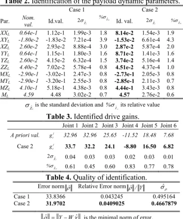
calculated using CAD software. They are given in table 2. Their values are accurate due to the simplicity of the payload shape (Fig. 2).
Two different identifications of the payload inertia parameters are achieved:
- Case 1: the payload parameters are identified using the manufacturer’s drive gains
- Case 2: the drive gains are first identified with the base parameters with IDIM-WTLS using the knowledge on the payload mass. They are then used in order to achieve a new identification of the new the payload parameters and the robot dynamic parameters with IDIM-WLS.
The manufacturer’s drive gains (Case 1) and the identified ones (Cases 2) are given in table 3. For each joint, the
identified values are close for the manufacturer’s values, but the mean error is about 9%. The maximal error grows up to 24%!
The identified values of the payload inertial parameters are presented in table 2. Moreover, the quality of identification is detailed at table 4. It appears that the identified gains lead to the best results. The efficiency and the simplicity of the method are really appealing, especially for industrial robots for which manufacturer’s gains are too often very difficult to obtain.
Finally, in order to validate the new drive gain values a new payload is identified (Table 5). The parameters are very close to the a priori ones in all cases. The torques calculated with the model (12) identified with the gains of Case 2 are presented in Fig. 3. It is possible to conclude that the drive gains have been well identified with the IDIM-WTLS.
5. CONCLUSION
This paper has presented a new method for the global identification of the total drive gains for robot joints. This method is easy to implement and does not need any special test or measurement on elements inside the joint drive train. It
Fig. 2. The 4.59 Kg payload
Table 2. Identification of the payload dynamic parameters.
Case 1 Case 2
Par. Nom. val. Id.val. 2 ˆi %ˆri Id. val. 2
i
ˆ
%ˆri
XXL 0.64e-1 1.12e-1 1.99e-3 1.8 8.14e-2 1.54e-3 1.9 XYL -1.80e-2 -1.83e-2 7.21e-4 3.9 -1.53e-2 6.61e-4 4.3 XZL 2.60e-2 2.93e-2 8.88e-4 3.0 2.87e-2 5.87e-4 2.0 YYL 0.64e-1 1.15e-1 1.80e-3 1.6 8.71e-2 1.41e-3 1.6 YZL 2.60e-2 4.15e-2 6.32e-4 1.5 3.74e-2 5.16e-4 1.4 ZZL 4.40e-2 7.02e-2 5.78e-4 0.8 4.51e-2 4.37e-4 1.0 MXL -2.90e-1 -3.02e-1 2.47e-3 0.8 -2.73e-1 2.05e-3 0.8 MYL -2.90e-1 -3.20e-1 2.55e-3 0.8 -2.85e-1 2.11e-3 0.7 MZL 4.10e-1 5.18e-1 4.38e-3 0.8 4.44e-1 3.43e-3 0.8 ML 4.59 4.48 3.02e-2 0.7 4.57 2.76e-2 0.6
i
ˆ
is the standard deviation and
ri
ˆ
% its relative value
Table 3. Identified drive gains.
Joint 1 Joint 2 Joint 3 Joint 4 Joint 5 Joint 6
A priori val. j g 32.96 32.96 25.65 -11.52 18.48 7.68 Case 2 j g 33.7 32.2 24.1 -8.80 16.50 6.82 2ˆi 0.04 0.03 0.03 0.02 0.03 0.01 ri ˆ % 0.61 0.45 0.60 0.83 0.77 0.78
Table 4. Quality of identification.
Error normˆ Relative Error norm ˆ / Y ˆ
Case 1 33.8366 0.043245 0.495164
Case 2 31.9702 0.0409025 0.4667879
ˆ Y Wˆ
is based on a IDIM-WTLS technique using current reference and position sampled data while the robot is tracking one reference trajectory without load fixed on the robot and one trajectory with a known payload fixed on the robot, whose inertial parameters are measured. The method has been experimentally validated on an industrial Stäubli TX-40 robot. Using the identified drive gains, the identification of the total dynamic model has been improved and another payload has been accurately identified. This shows the effectiveness of the method.
ACKNOWLEDGEMENTS
This work is supported by the French grant FUI IRIMI F1004026 Z.
REFERENCES
Corke, P. (1996). In situ measurement of robot motor electrical constants. Robotica, Vol. 23, No. 14, pp. 433–436.
Featherstone, R. and Orin, D.E. (2008). Dynamics – chapter 2. In Siciliano B. and Khatib O. eds Springer Handbook of Robotics. Gautier, M. (1991). Numerical calculation of the base inertial
parameters. Journal of Robotics Systems, Vol. 8, No. 4, pp. 485–506.
Gautier, M. (1997). Dynamic identification of robots with power model. In: Proc. IEEE ICRA, Albuquerque, USA, April, pp. 1922–1927.
Gautier, M. and Briot, S. (2011). New method for global identification of the joint drive gains of robots using a known inertial payload. Proc. IEEE ECC CDC, December 12-15, Orlando, Florida, USA.
Gautier, M. and Briot, S. (2011). New method for global identification of the joint drive gains of robots using a known payload mass. In: Proc. IEEE IROS, Sept., San Fran., USA. Gautier, M. and Khalil, W. (1990). Direct calculation of minimum
set of inertial parameters of serial robots. IEEE Trans. on
Robotics and Automation, Vol. 6, No. 3, pp. 368-373.
Gautier, M., Vandanjon, P. and Presse, C. (1994). Identification of inertial and drive gain parameters of robots. In: Proc. IEEE
CDC, Lake Buena Vista, FL, USA, pp. 3764–3769.
Golub, G.H. and Van Loan, C.F. (1996). Matrix computation. J.
Hopkins 3rd Ed.
Hollerbach, J., Khalil, W. and Gautier, M. (2008). Model identification – Chapter 14. In Siciliano B. and Khatib O. eds
Springer Handbook of Robotics.
Khalil, W. and Dombre, E. (2002). Modeling, identification and control of robots. Hermes Penton London.
Khalil, W., Gautier, M. and Lemoine, P. (2007) Identification of the payload inertial parameters of industrial manipulators. In:
Proc. IEEE ICRA, Roma, Italy, April 10-14, pp. 4943–4948.
Khosla, P.K. and Kanade, T. (1985). Parameter identification of robot dynamics. In: Proc. 24th IEEE CDC, Fort-Lauderdale, pp. 1754–1760.
Lu, Z., Shimoga, K.B. and Goldenberg, A. (1993). Experimental determination of dynamic parameters of robotic arms. Journal
of Robotics Systems, Vol. 10, No. 8, pp.1009–1029.
Mayeda, H., Yoshida, K. and Osuka, K. (1990). Base parameters of manipulator dynamic models. IEEE Trans. on Robotics and
Automation, Vol. 6, No. 3, pp. 312–321.
Restrepo, P.P. and Gautier, M. (1995). Calibration of drive chain of robot joints. In: Proc. 4th IEEE Conference on Control
Applications, pp. 526–531.
Van Huffel, S. and Vandewalle, J. (1991). The total least squares problem: computational aspects and analysis. In: Frontiers in
Applied Mathematics series, 9. Philadelphia, Pennsylvania:
SIAM. 0 2 4 6 8 10 −100 −80 −60 −40 −20 0 20 40 60 80 Time (s) Motor torque (N ⋅ m) Joint 1 Measure=Y Estimation=W X Error=Y−W X 0 2 4 6 8 10 −150 −100 −50 0 50 100 Time (s) Motor torque (N ⋅ m) Joint 2 Measure=Y Estimation=W X Error=Y−W X 0 2 4 6 8 10 −80 −60 −40 −20 0 20 40 60 Time (s) Motor torque (N ⋅ m) Joint 3 Measure=Y Estimation=W X Error=Y−W X 0 2 4 6 8 10 −15 −10 −5 0 5 10 15 20 Time (s) Motor torque (N ⋅ m) Joint 4 Measure=Y Estimation=W X Error=Y−W X 0 2 4 6 8 10 −40 −30 −20 −10 0 10 20 30 Time (s) Motor torque (N ⋅ m) Joint 5 Measure=Y Estimation=W X Error=Y−W X 0 2 4 6 8 10 −15 −10 −5 0 5 10 15 20 Time (s) Motor torque (N ⋅ m) Joint 6 Measure=Y Estimation=W X Error=Y−W X
Fig. 3. Measured and computed torques of the TX-40 with the payload of 4.59 kg. Table 5.
Identification of the new payload dynamic parameters.
Case 1 Case 2
Par. Nom. val. Id.val. 2 ˆi %ˆri Id. val. 2 ˆi %ˆri
XXL 1.51e-2 1.57e-2 8.75e-4 5.6 1.11e-2 8.07e-4 7.2 XYL -9.06e-4 -2.41e-3 3.16e-4 13.1 -2.08e-3 2.79e-4 13.4 XZL 3.61e-3 4.21e-3 3.34e-4 7.9 4.11e-3 2.94e-4 7.1 YYL 1.51e-2 1.40e-2 8.95e-4 6.4 1.13e-2 7.57e-4 6.7 YZL 3.61e-3 1.93e-3 3.00e-4 15.5 1.49e-3 2.66e-4 17.9 ZZL 3.44e-3 3.88e-3 2.88e-4 7.4 1.34e-3 2.88e-4 21.5 MXL -4.00e-2 -2.37e-2 1.59e-3 4.7 -2.74e-2 1.30e-3 4.8 MYL -3.99e-2 -4.18e-2 1.41e-3 3.4 -3.90e-2 1.31e-3 3.3 MZL 0.15 0.192 2.51e-3 1.3 0.166 2.22e-3 1.3 ML 1.686 1.66 1.74e-2 1.0 1.66 1.73e-2 1.0
i
ˆ
is the standard deviation and
ri
ˆ