Performance enhancement of a BSDF test bench using an algorithm
fed with laser-tracker measurements
L. Clermont*
a, C. Michel
a, E. Mazy
a aCentre Spatial de Liège (CSL), STAR Institute, Avenue du Pré-Aily, 4031 Angleur, Belgium
ABSTRACT
In the field of earth-observation, on-board calibration is often necessary to guarantee the radiometric accuracy of space instruments. A typical method is to use large diffusers in front of the instrument, illuminated with a reference source like the sun [1]. Hence, it is necessary to characterize the scattering properties of the diffuser with excellent accuracy. Given the large size and weight of the diffusers to characterize, CSL have developed a bench which uses a robot arm to manipulate the sample. For the most stringent applications, the typical accuracy of robotic arms is not good enough to measure the BSDF with a satisfactory accuracy. A method have been developed which uses laser tracker measurements of the sample during a calibration phase and compensate for the robot errors. This paper describes the principle of the method and the results obtained. We also present the model of how the orientation error of the sample affects the BSDF relative error.
Keywords: BSDF, BTDF, Bidirectional scattering distribution function, laser tracker, diffuser, calibration
1. INTRODUCTION
In the field of earth-observation, on-board calibration is often necessary to guarantee the radiometric accuracy of space instruments. A typical method is to use large diffusers in front of the instrument, illuminated with a reference source like the sun [1]. Hence, it is necessary to characterize the scattering properties of the diffuser with excellent accuracy. Given the large size and weight of the diffusers to characterize, CSL have developed a bench which uses a robot arm to manipulate the sample. For the most stringent applications, the typical accuracy of robotic arms is not good enough to measure the BSDF with a satisfactory accuracy. A method have been developed which uses laser tracker measurements of the sample during a calibration phase and compensate for the robot errors. This paper describes the principle of the method and the results obtained. We also present the model of how the orientation error of the sample affects the BSDF relative error.
2. BSDF BENCH DESCRIPTION
Experimentally, the BSDF can be measured by illuminating a sample at a given angle of incidence and measuring the scattered light at different angles [2][3]. The equation below is then used, where Sscat is the measured scattering signal, Ssrc is the measured incident beam reference signal and is the solid angle of the detector when viewed from the sample [4]. The angles are considered in spherical coordinates with respect to the sample, as illustrated on Figure 2.
(
)
(
)
(
)
(1)
The 3D CAD model of the CSL BSDF bench is shown on Figure 1. The main elements are the source block, detector block, and the manipulator (robot arm) which holds the sample. The source block generates a quasi-collimated beam to illuminate the sample. The detector block rotates around a vertical axis and is meant to measure the scattered light at different angles from incidence direction. The combination of rotation of the detector and robot motion allows measuring Sscat for different values of (θi, Φi, θs, Φs) [5].
Figure 1: CAD model of the BSDF test bench at CSL
Figure 2: Convention for the definition of the angles (θi, Φi, θs, Φs)
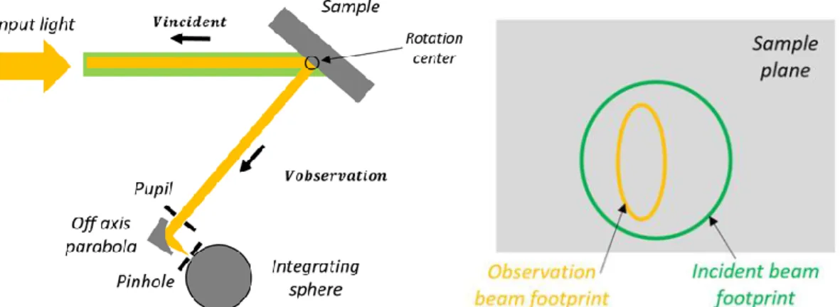
Figure 3-left here-after shows a simplified sketch of the test setup. The detector block uses an off-axis parabola followed by a pin-hole which restricts angularly the light which enters in the integrating sphere and is measured. Furthermore, a pupil is placed in front of the off-axis mirror to limit spatially the zone of the sample at which the BSDF is measured. Consequently, even in the case where the incident beam would have a large footprint at the sample, the pupil restricts the observation beam footprint to a smaller zone (Figure 3-right).
Figure 3 : (Left) Simplified sketch of the BSDF test setup (in reflective configuration, BRDF). (Right) Overlap of the observation and incident beams footprints on the sample
3. ERROR MODEL
If the angles (θi, Φi, θs, Φs) are affected by the errors dθi, dΦi, dθs and dΦs, the absolute error on the BSDF is obtained by computing the total derivative with respect to the angles (angles considered in radians):
(2)
By using equation (1), the expression can be developed as follows:
(
(
)
)
(
)
(3)
The relative error thus takes the following form:
(
)
(
)
(4)
In the expression of the relative error, the first term is the only one to be independent of the scattering profile. This is a term which will always be present, whatever the scattering profile, and represents the minimum error for any scattering profile. In the particular case of a uniform BSDF profile, all the other terms are equal to zero. Already with this term alone, an error on the orientation could lead to a significant relative error on the BSDF. The Figure 4 shows in that case how the relative BSDF error evolves with the incidence angles, considering different values for the error dθi. As it shows, the relative error on the BSDF is very small close to normal incidence but increases very fast with the incidence angle. For example, in the case where dθi=5.8’=350’’, the error on the BSDF would be 0.17% at 45°, 0.47% at 70°.
Figure 4: Relative BSDF error as a function of the incidence angle, for different error on the incidence angle, considering a sample with scattering profile lambertian and with invariant hemi reflectance
For non-uniform BSDF profiles, the other terms will also contribute to an error in a way which is to calculate on a case by case basis as it depends on the type of profile. In particular, the error will be the larger when the profile varies rapidly with the angles. A simple case to derive is the perfect Lambertian emitter. In that case, the profile is symmetrical around the azimuthal direction and thus the terms ⁄ and ⁄ vanishes. Also, the term ⁄ is equal to
zero when the total integrated reflectance is invariant with the incidence angle. In that condition, the last non zero term which depends on the scattering profile is the one involving the derivative with respect to the scattering angle. As
( ) for a Lambertian emitter, the equation below is obtained for the total error. As it shows, the relative
error increases when the incidence angle or scatter angle increases. Figure 5 shows the error as a function of θi and θs, considering an error on both angles of 350’’. In that case, for example, the relative error is 0.24% when θi=θs=45° and reaches 0.66% for θi=θs=70°. Let’s however mention that in practice the errors on the angles are (non-independent) random variables, which means that the sum of equation (5) is actually to be seen as a RSS sum, which will give a result smaller than the algebraic sum.
(
) (
)
(
)
(5)
Figure 5 : Relative BSDF error for a Lambertian sample with invariant total integrated scattering (limited to 75° incidence and scatter angle), considering an error on the angles of 350’’
Typically, the robot arm used at CSL gives orientation errors of more than 350’’. When the desired BSDF required error is supposed to be <0.2%, this means that at large angles it would not be possible to perform the characterization with error low enough if nothing is done to improve the orientation accuracy. This thus justifies the method developed here.
4. BENCH CHARACTERIZATION
4.1 Reference frames
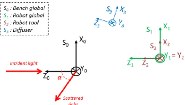
4 orthonormal reference frames are defined and labeled S0 to S3 (Figure 6). By convention, a vector V defined in reference frame Si is labeled Vi. S0 is the reference frame of the BSDF test bench and have its X and Y axis approximately horizontal. This is the frame in which the incident light direction and observation direction is characterized. The robot is placed on the bench and defines a reference frame S1 which is constant in S0. The robotic arm is characterized by reference frame S2 and moves with respect to S1. It is the movement of S2 relative to S1 which is considered when giving the instructions to the robot. The sample to measure is placed on a tool at the end of the robotic arm, it defines a reference frame S3 which is fixed in S2.
Figure 6 : Reference frames in the BSDF bench
Each reference frame is physically represented by at least 3 non co-aligned retro-reflective beads (SMR, spherically mounted retro-reflector). A laser tracker can be used to measure the position of the different SMR, either in interferometric mode or in time of flight mode. From the position of the beads, the axis (X,Y,Z) of a reference frame can be defined systematically. The characterization accuracy of a reference frame thus depends on the accuracy with which each SMR is measured. The error on the position measurement of a SMR depends on parameters such as the size of the SMR or the type and configuration of the laser tracker. Typically, a laser tracker in interferometric mode will measure the SMR position with an error of ±A=10µm, while in time of flight mode A=20µm. A rule of thumb to estimate the orientation error of a reference frame is to use the equation below. This equation indeed calculate the tilt of a straight line between two SMR spaced by L, whose lateral positions are affected by a statistical ±A and thus where the total lateral error is the RSS sum of A, leading to the square root of 2 term.
(
√
)
(6)
(7)
Instruction to the robot are given from S2 to S1, however the incident and observation vectors are known in S0 and the angles (θi, Φi, θs, Φs) defines vectors in S3. Consequently, when calculating the rotation and translation matrix which must be applied to position the sample, the operation is affected by the characterization error of each of the 4 reference frames. The total error is hence obtained by calculating the RSS sum of the error of the individual reference frames, as shown on equation below and gives the performance limit due to characterization.
√∑
√∑ (
√
)
(9)
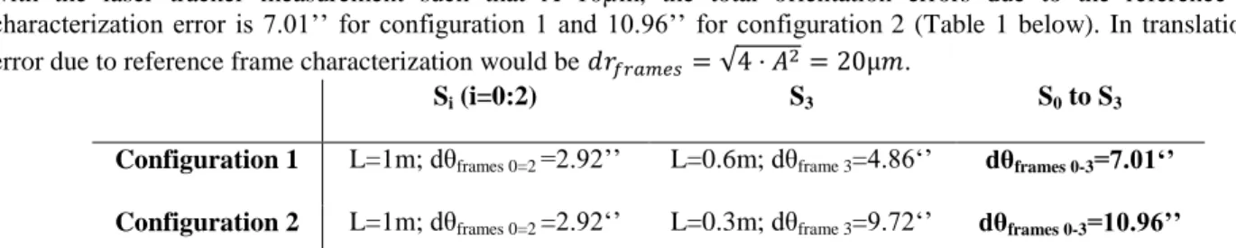
In the case of the CSL bench, the distance L is about 1m for S0 to S2. For the reference frame of the sample, S3, the distance depends on the size of the sample: two configurations are considered, L≈0.3m or L≈0.6m. In that condition and with the laser tracker measurement such that A=10µm, the total orientation errors due to the reference frame characterization error is 7.01’’ for configuration 1 and 10.96’’ for configuration 2 (Table 1 below). In translation, the error due to reference frame characterization would be √ .
Si (i=0:2) S3 S0 to S3
Configuration 1 L=1m; dθframes 0=2 =2.92’’ L=0.6m; dθframe 3=4.86‘’ dθframes 0-3=7.01‘’
Configuration 2 L=1m; dθframes 0=2 =2.92‘’ L=0.3m; dθframe 3=9.72‘’ dθframes 0-3=10.96’’
Table 1 : Accuracy limit due to reference frame characterization orientation error
4.2 Incident and observation vectors
It is necessary to characterize the coordinates of the incident beam direction, , as well as the coordinates of the observation beam direction as a function of the detector block rotation angle β, ( ). The characterization is done at the moment where the test setup is aligned. A theodolite is used which provides the vectors coordinates in its own reference frame.
For the observation direction, the first step of the characterization consists in finding the rotation axis of the detector block. For that, an SMR is placed on the detector block and its position is measured as a function of the detector block angle. The SMR position describes a circle in the 3D space, its center is the rotation center of the block and the normal to the circle is the axis. Tip tilt stages are used to adjust the rotation center on the X axis of S0. The SMR is then placed at the rotation axis, manually moving its position up to the point where it stays constant (within laser tracker measurement accuracy) when the detector block rotates. Next, the detector block is kept at a fixed angle β* and a theodolite is used to point toward the rotation axis, materialized by the SMR, and simultaneously approximately toward the pin-hole of the detector block. At that point, the pin-hole is finely adjusted and the theodolite gives the coordinates of ( ). At other angles β, the wobble is characterized to determine the deviation of the observation
vector normal to the plane of rotation. Ultimately, this characterization step provides the coordinates ( ) as a function of the detector block angle. The incident beam is aligned so that it goes through
the rotation axis of the detector block. Its characterization is then immediate to do with a theodolite and provides . Ultimately it is necessary to get the vector coordinates in the reference frame S0, thus the reference frame of the theodolite is to be measured in S0. This is done by placing a mirror in autocollimation with respect to the theodolite and measuring the position of SRMs with a tracker in direct view and through the mirror. At the end of these operations, the coordinate and ( ) is known, and the angle between these two vectors can be computed as a function of the detector block angle:
( ) (
( ))
(10)
In the theodolite reference frame, the error on the characterization of the incident vector comes only from the error from the theodolite, . For the observation vector, another source of error is the position of the rotation center (±A, the error on the measurement of its position with the laser tracker). Hence, when the theodolite points toward the SRM, the error A induce a pointing error of ( ⁄ ) where l is the distance from theodolite to SRM. Consequently, the observation vector error in the theodolite reference frame is the root squared sum of and as these terms are
independent, while for the incident vector the error is . The error associated to the change of basis from theodolite
reference frame to S0 operation is the RSS sum of (autocollimation error) and ( ⁄ ), where L is the distance
between the SRM and its image through the mirror, and A* is the measurement error. For practical reason, the tracker must be used in time of flight mode, giving a larger error on A* than in interferometric mode. Considering typical values for the BSDF bench at CSL ( , A=10µm; l=2m; A*= 20m; L=2m), the characterization error is dθcharac≈4.5‘’.
5. BENCH CONTROL
5.1 Theoretical alignment
The sample reference frame S3 is initially at home position. From the angle (θi; φi; θr; φr), we define what the coordinates must be for the incident and observation vectors (Vinc, Vobs) in the diffuser reference frame S3:
(
(
) (
)
(
) (
)
(
)
)
(
(
) (
)
(
) (
)
(
)
)
(11)
From there, angle α between these two vectors can be calculated. From the characterization of incident and observation vectors in S0 which gave the relationship between α and β (equation (10)), this directly tells how much the detector block must be rotated.
(
)
(12)
Ultimately, the goal of the operation is to co-align with and with and to position the sample at the detector block rotation center. For the orientation, the process to execute with the robotic arm is the combination of two rotation. A first rotation is meant to align Vinc with Vincident: the diffuser is rotated around a vector perpendicular to these two vectors. Then, a second rotation is performed around Vincident and is meant to align Vobs with Vobservation. Each rotation can be described with a rotation matrix, R1 and R2 respectively: the total operation corresponds to the matrix multiplication Rtot=R1∙R2. If u= [u(1) u(2) u(3)] is the rotation axis and γ is the rotation angle, then the rotation matrix R writes as shown below.
( ( ) ( ( ) ) ( ) ( ) ( ) ( ) ( ) ( ) ( ) ( ) ( ) ( ) ( ) ( ) ( ) ( ( ) ) ( ) ( ) ( ) ( ) ( ) ( ) ( ) ( ) ( ) ( ) ( ) ( ) ( ) ( ( ) ) )
(13)
Where c and s are defined as: ( ) and ( )
The calculation of the rotation matrix is performed in reference frame S1 as this is the reference for the robot. Hence, change of basis is performed for all vectors. Rotation matrices R1 and R2 are obtained with the parameters of table below. The vectors considered for the computation of parameters of the first rotation are the initial coordinates. For the second rotation, the parameters are computed after applying the matrix R1 to vinc and vobs.
Rotation 1:
Rotation 2:
(
)
(
)
(14)
For the translation matrix, the rotation matrix R is applied to the initial position of S3 and the difference with target position (i.e. detector block rotation center) is computed.
(15)
Once the rotation and translation matrix is computed, the robotic arm is moved with those parameters (rotation matrix is entered as Euler angles). At this stage, the geometrical error comes from the error on the characterization of the reference frames, incident and observation angles, center or rotation and of course the robot itself.
5.2 Fine control
Once the theoretical positioning of the sample is performed, the laser tracker is used to measure the actual position and orientation of S3. When the positioning accuracy is not satisfactory, an additional step is added to the previous to compensate from the deviation.
The principle is to calculate the theoretical rotation matrix which should be applied to the real measured coordinates of S3 so that it reaches the desired correct orientation. For that, the same principle as above is computed but considering for S3 the measured coordinates after displacement instead of the home coordinates. If Rcorr is the resulting compensation rotation matrix, the total rotation matrix is then R’=R1R2Rcorr. That matrix R’ is used as the new input for the robot, as it always consider positioning with respect to its home position. If after that step the accuracy is still not satisfactory, the process of compensation can be reproduced iteratively. For the translation error compensation, the principle is simply to add to the translation matrix the difference of coordinates between the target position and the actual position as it is after the iterations of orientation compensation.
(
)
(16)
(17)
The measurement of the BSDF usually implies a very large number of different fields (θi; φi; θr; φr). Hence, it would be time consuming to compute the compensation matrices to apply for every situation. For that reason, the principle is to calibrate only once the compensation matrix for a limited number of fields. Each time a measurement of the BSDF is performed for a given field, the compensation matrix of the closest neighboring field is applied.
After theoretical alignment, the sample is affected by an orientation error which contains both the intrinsic robot error and . After the compensation process, decreases but cannot be lower than as
(18)
Finally, the error on the angles (θi; φi; θr; φr) is affected by both the control error and the characterization error of the incident and observation vectors in S0. Hence, as those errors are independent we write:
√
(19)
6. PERFORMANCE RESULTS
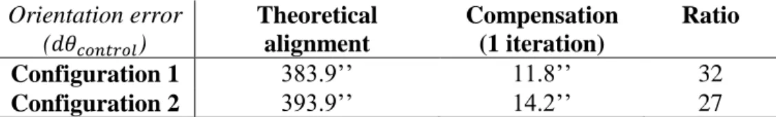
The robotic arm was displaced at different positions, associated to different angles for the BSDF measurement. The reference frame S3 was then measured with the laser tracker to provide the input for the compensation process. Table 2 below shows the orientation statistical error for the theoretical alignment as well as after compensation (errors on the axis (X, Y, Z) which defines S0 and for the different situations of angles considered). As the Table 2 below shows, the initial orientation error is very large with about 390’’. After an iteration of orientation compensation, the error is decreased down by a factor of about 30. If the contribution of is removed from , we get that the robot is able
after 1 compensation to orient a sample with an accuracy of 10’’ for both configuration 1 and 2.
Orientation error
(
)
Theoretical
alignment
Compensation
(1 iteration)
Ratio
Configuration 1
383.9’’
11.8’’
32
Configuration 2
393.9’’
14.2’’
27
Table 2: Orientation error of the sample before and after compensation
By using equation (19) and the value of dθsharac derived earlier, we get that the after compensation the statistical error on the angles (θi, Φi, θs, Φs) is respectively 12.6’’ and 14.9’’ for configurations 1 and 2. This is a significant improvement compared to the situation of the theoretical alignment which yields a significant improvement of the BSDF measurement accuracy. For example, in the case of a Lambertian diffuser at θi=θs=70°, equation (5) gives that the BSDF relative error would be 0.028% if the error is 14.9’’ for both dθi and dθs.
7. CONCLUSIONS
Characterizing the scattering properties of large scale diffusers is necessary when it comes to on-board calibration of space instruments. The large size and weight of the samples to characterize however require hardware materials (robot arm) which intrinsically have insufficient accuracies. We have demonstrated analytically how such errors impact the BSDF measurement. In particular, the relative BSDF error scales linearly with the orientation error of the robot arm. A method have been developed which uses laser tracker calibration measurements to feed an algorithm which compensate for the errors. While the orientation error was very large initially, up to about 390’’, a reduction of the orientation error by about a factor is 30 is obtained.
REFERENCES
[1] L. Clermont et al., "Design and tests of the sun baffle for the Sentinel-4 UVN embedded calibration assembly", Proc. SPIE 10562, International Conference on Space Optics — ICSO 2016, 1056201 (25 September 2017) [2] J. Stover, "Optical Scattering: Measurement and Analysis", SPIE press book (2012)
[3] E.C Fest, “Stray-light analysis and control”, SPIE press
[4] J.Y. Plesseria et al., “Development of a BRDF measurement bench for characterisation of diffuse reflective materials”, Proc. 12th European Conference on Space Structures, Materials & Environmental testing”, 2012 [5] E. Mazy et al., “Recent development in BTDF/BRDF metrology on large-scale lambertian-like diffusers,
application to on-board calibration units in space instruments”, Proc. SPIE 11056-48 (2019) [6] P. A Lightsey, “Systems Engineering for Astronomical Telescopes”, SPIE press book (2018)