2012 — Improving evolutionary algorithms by MEANS of an adaptive parameter control approach

(1)

ÉCOLE DE TECHNOLOGIE SUPÉRIEURE UNIVERSITÉ DU QUÉBEC

MANUSCRIPT-BASED THESIS PRESENTED TO

ÉCOLE DE TECHNOLOGIE SUPÉRIEURE

IN PARTIAL FULFILLEMENT OF THE REQUIREMENTS FOR THE DEGREE OF DOCTOR OF PHILOSOPHY

Ph. D.

BY

Guillaume CORRIVEAU

IMPROVING EVOLUTIONARY ALGORITHMS BY MEANS OF AN ADAPTIVE PARAMETER CONTROL APPROACH

MONTREAL, DECEMBER 7 2012 Guillaume Corriveau, 2012

(2)

This Creative Commons licence allows readers to download this work and share it with others as long as the author is credited. The content of this work can’t be modified in any way or used commercially.

(3)

BOARD OF EXAMINERS (THESIS PH.D.)

THIS THESIS HAS BEEN EVALUATED

BY THE FOLLOWING BOARD OF EXAMINERS

Mr. Raynald Guilbault, Thesis Supervisor

Mechanical Engineering Department at École de technologie supérieure

Mr. Antoine Tahan, Thesis Co-supervisor

Mechanical Engineering Department at École de technologie supérieure

Mr. Robert Sabourin, Thesis Co-supervisor

Automated Production Engineering Department at École de technologie supérieure

Mr. Simon Joncas, President of the Board of Examiners

Mr. Tony Wong, Member of the jury

Mr. Sébastien Adam, External Evaluator LITIS laboratory

Université de Rouen

THIS THESIS WAS PRENSENTED AND DEFENDED

IN THE PRESENCE OF A BOARD OF EXAMINERS AND PUBLIC ON OCTOBER 30, 2012

(4)

(5)

FOREWORD

Since this research is shaped as a manuscript-based thesis, there is some duplication across chapters. In fact, four of the five chapters have already been submitted as self-content papers. Nonetheless, special effort has been paid throughout the writing of these manuscripts to ensuring continuity to the best extent possible. Consequently, from the author’s perspective, these repetitions do not detract from the purpose of the thesis, but rather help to strengthen important concepts.

(6)

(7)

ACKNOWLEDGMENT

I would like to thanks my thesis advisor, Raynald Guilbault, Antoine Tahan and Robert Sabourin, for their technical, financial, and moral support throughout these years. Their guidance was always fruitful and their interest in this research project always encouraged me to push my own limit. I am also grateful for the freedom they provided to me. Many thank to Simon Joncas, Tony Wong, and Sébastien Adam for their participation to the board of examiners.

Also, I am grateful to the Fonds de recherche du Québec – Nature et technologies (FQRNT), Rio Tinto Alcan, and the École de technologie supérieure for their financial contribution to this research project.

Special thank go to Cynthia Orman for her assistance on the language correction. I am beholden to her as well as to Raynald Guilbault for the language quality of this thesis.

In addition, I would like to express my gratitude to my employer, Bombardier aerospace, and more specifically to my immediate superior, Franck Dervault, for the constant support in the last two years. They have shown understanding that led me the required flexibility to successfully complete this research project.

I would like to thank my parents who inspired me with their guidance and open mind. Finally, I am indebted to my beloved partner, Marjorie Leduc, for her patience, support, and encouragement during all these years. I cannot express in word all the gratitude I have regarding the sacrifices she made to follow me in this very demanding adventure. Thank to my daughter, Anaïs, who gave me the motivation during hard days. Together, they have skillfully succeeded to keep me in touch with real life.

With the hope that I will now be able to master the exploration/exploitation balance in my own life!

(8)

(9)

IMPROVING EVOLUTIONARY ALGORITHMS BY MEANS OF AN ADAPTIVE PARAMETER CONTROL APPROACH

Guillaume CORRIVEAU

RÉSUMÉ

Les algorithmes évolutionnaires (AE) représentent une classe de méthodes d’optimisation couramment employée afin de résoudre divers problèmes scientifiques complexes. Cependant, les AE convergent souvent prématurément sur un optimum local, le processus évolutif est coûteux et les paramètres internes des AE sont difficilement réglables. Afin de pallier à ces problématiques et améliorer la performance des AE, il nous apparaît nécessaire d’aborder en premier lieu la question du réglage des paramètres. Pour ce faire, l’objectif de la thèse est de développer une méthode adaptative apte à contrôler l’ensemble des paramètres des AE, et ce, en utilisant comme indicateur de rétroaction le concept d’exploration et d’exploitation permettant d’interpréter le chemin de recherche poursuivi par l’optimiseur. Ainsi, le système adaptatif permettra de guider l’optimiseur vers sa direction de recherche optimale, ce qui offrira la possibilité de réduire le phénomène de convergence prématurée et qui devrait influencer positivement les coûts de calcul du processus évolutif.

Dans un premier temps, afin de caractériser l’exploration de l’espace de recherche offert par l’optimiseur, les mesures de diversité génotypique disponibles sont revues et étudiées. Pour ce faire, un banc d’essai spécialement dédié à cette fin est introduit et trois critères de diversité sont proposés pour évaluer la pertinence de ces mesures en tant qu’indicateur de diversité d’une population. Les résultats de cette étude montrent qu’aucune formulation publiée à ce jour n’est en mesure d’estimer adéquatement la diversité. Ce faisant, une nouvelle formulation génotypique est développée et l’analyse de ses performances révèle qu’elle offre généralement une meilleure description de la diversité malgré le fait qu’elle possède certaines lacunes importantes.

Pour caractériser l’exploitation des zones prometteuses pourvues par l’optimiseur, une étude similaire est conduite. Néanmoins, elle est maintenant orientée sur les mesures de convergence phénotypique disponibles puisque l’exploitation est principalement représentée par la réponse des individus. Encore une fois, l’analyse détaillée révèle qu’aucun descripteur phénotypique publié à ce jour n’est susceptible de représenter adéquatement la distribution de solutions d’une population donnée. Par conséquent, une nouvelle formulation phénotypique est développée dans le cadre de cette thèse et une analyse approfondie montre que cet indicateur exprime parfaitement le comportement escompté, et ce, en suivant une variété de populations.

Inspirés par ces réalisations, nous introduisons un outil de diagnostic basé sur la nouvelle formulation génotypique et phénotypique. L’utilité de cet outil est illustré en comparant l’impact que peut engendrer divers paramètres des AE sur le processus de recherche. Bien

(10)

que le but principal de ce développement soit d’exposer la pertinence d’employer à la fois une mesure génotypique et une mesure phénotypique pour caractériser le processus de recherche, l’outil de diagnostic s’avère être l’un des rares outils à la disposition des utilisateurs des AE permettant d’améliorer le processus de recherche sur des problèmes d’optimisation réels.

Sur la base des connaissances acquises, l’objectif principal de cette thèse est finalement considéré par la mise en place d’une nouvelle approche adaptative permettant de contrôler les paramètres des AE. La proposition est fondée sur l’utilisation d’un réseau Bayesien permettant d’interagir simultanément sur l’ensemble des paramètres des AE. À notre connaissance, il s’agit du premier système adaptatif offrant de telles capacités. En ce qui concerne le schéma de récompense employé par le système pour juger de la productivité des paramètres, les mesures génotypique et phénotypique développées précédemment sont mises à contribution, et ce, en favorisant les paramètres offrant une maximisation de l’exploration et de l’exploitation. La performance de ce système est analysée à l’aide d’un algorithme génétique à état constant (SSGA), et ce, sur un banc d’essai reconnu dans le domaine (CEC’05). De plus, cette nouvelle approche est comparée à sept autres méthodes, dont FAUC-RMAB et G-CMA-ES représentant actuellement l’état de l’art en terme de système adaptatif. Dans l’ensemble, les résultats montrent statistiquement que l’approche proposée est comparable à G-CMA-ES et qu’elle surpasse la plupart des autres méthodes adaptatives. Toutefois, cette étude expose le fait qu’aucune des méthodes considérées n’est capable de localiser l’optimum global sur des problèmes hautement multimodaux. Ceci nous conduit à affirmer qu’il y a sans doute un manque de synergie et de complémentarité entre les différents paramètres impliqués.

Par conséquent, nous recommandons la poursuite des recherches sur ces thèmes avec la perspective d’obtenir de meilleurs algorithmes d’optimisation. Pour ce faire, diverses recommandations sont proposées à la fin de cette thèse.

Mots-clés : contrôle adaptatif des paramètres, mesures de diversité, algorithmes évolutionnaires, équilibre entre exploration/exploitation, convergence prématurée

(11)

IMPROVING EVOLUTIONARY ALGORITHMS BY MEANS OF AN ADAPTIVE PARAMETER CONTROL APPROACH

Guillaume CORRIVEAU ABSTRACT

Evolutionary algorithms (EA) constitute a class of optimization methods that is widely used to solve complex scientific problems. However, EA often converge prematurely over suboptimal solutions, the evolution process is computational expensive, and setting the required EA parameters is quite difficult. We believe that the best way to address these problems is to begin by improving the parameter setting strategy, which will in turn improve the search path of the optimizer, and, we hope, ultimately help prevent premature convergence and relieve the computational burden. The strategy that will achieve this outcome, and the one we adopt in this research, is to ensure that the parameter setting approach takes into account the search path and attempts to drive it in the most advantageous direction. Our objective is therefore to develop an adaptive parameter setting approach capable of controlling all the EA parameters at once. To interpret the search path, we propose to incorporate the concept of exploration and exploitation into the feedback indicator.

The first step is to review and study the available genotypic diversity measurements used to characterize the exploration of the optimizer over the search space. We do this by implementing a specifically designed benchmark, and propose three diversity requirements for evaluating the meaningfulness of those measures as population diversity estimators. Results show that none of the published formulations is, in fact, a qualified diversity descriptor. To remedy this, we introduce a new genotypic formulation here, the performance analysis of which shows that it produces better results overall, notwithstanding some serious defects.

We initiate a similar study aimed at describing the role of exploitation in the search process, which is to indicate promising regions. However, since exploitation is mainly driven by the individuals’ fitness, we turn our attention toward phenotypic convergence measures. Again, the in-depth analysis reveals that none of the published phenotypic descriptors is capable of portraying the fitness distribution of a population. Consequently, a new phenotypic formulation is developed here, which shows perfect agreement with the expected population behavior.

On the strength of these achievements, we devise an optimizer diagnostic tool based on the new genotypic and phenotypic formulations, and illustrate its value by comparing the impacts of various EA parameters. Although the main purpose of this development is to explore the relevance of using both a genotypic and a phenotypic measure to characterize the search process, our diagnostic tool proves to be one of the few tools available to practitioners for interpreting and customizing the way in which optimizers work over real-world problems.

(12)

With the knowledge gained in our research, the objective of this thesis is finally met, with the proposal of a new adaptive parameter control approach. The system is based on a Bayesian network that enables all the EA parameters to be considered at once. To the authors’ knowledge, this is the first parameter setting proposal devised to do so. The genotypic and phenotypic measures developed are combined in the form of a credit assignment scheme for rewarding parameters by, among other things, promoting maximization of both exploration and exploitation. The proposed adaptive system is evaluated over a recognized benchmark (CEC’05) through the use of a steady-state genetic algorithm (SSGA), and then compared with seven other approaches, like FAUC-RMAB and G-CMA-ES, which are state-of-the-art adaptive methods. Overall, the results demonstrate statistically that the new proposal not only performs as well as G-CMA-ES, but outperforms almost all the other adaptive systems. Nonetheless, this investigation revealed that none of the methods tested is able to locate global optimum over complex multimodal problems. This led us to conclude that synergy and complementarity among the parameters involved is probably missing.

Consequently, more research on these topics is advised, with a view to devising enhanced optimizers. We provide numerous recommendations for such research at the end of this thesis.

Keywords: Adaptive parameter control, diversity measures, evolutionary algorithms, exploration/exploitation balance, premature convergence.

(13)

TABLE OF CONTENTS Page INTRODUCTION ...1 0.1 Background ...1 0.2 Research problem ...4 0.3 Objective ...8 0.4 Organization ...9

CHAPTER 1 REVIEW AND STUDY OF GENOTYPIC DIVERSITY MEASURES FOR REAL-CODED REPRESENTATIONS ...13

1.1 Introduction ...13

1.2 Genotypic diversity measure ...16

1.2.1 General concept ... 16

1.2.2 Normalization ... 17

1.2.3 Genotypic diversity measures ... 18

1.2.4 Prior observable flaws on certain GDMs ... 22

1.3 Review of comparative studies ...23

1.4 Benchmark ...25

1.5 Results ...28

1.5.1 Unimodal landscape experiment ... 29

1.5.2 Multimodal landscape experiment ... 32

1.5.3 Stability analysis ... 36

1.5.4 Sensitivity analysis... 37

1.5.5 Effect of outliers ... 40

1.6 GDM comparison over the CEC’05 benchmark ...43

1.7 Discussion ...47

1.8 Conclusion ...50

CHAPTER 2 EVALUATION OF GENOTYPIC DIVERSITY MEASUREMENTS EXPLOITED IN REAL-CODED REPRESENTATION ...51

2.2 Problem statement ...55

2.3 Characterizing population diversity ...59

2.4 Validation of the representative GDMs ...62

2.4.1 Reduced population arrangement ... 62

2.4.2 Controlled cases of population diversity ... 64

2.4.3 Discussion ... 67

CHAPTER 3 REVIEW OF PHENOTYPIC DIVERSITY FORMULATIONS FOR DIAGNOSTIC TOOL ...71

(14)

3.3 Review of phenotypic formulations ...76

3.3.1 General concept ... 77

3.3.2 Normalization ... 77

3.3.3 PCM formulation ... 79

3.4 Validation of phenotypic formulations ...82

3.4.1 Requirements for a suitable diversity measure ... 82

3.4.2 Validation framework for the requirements analysis ... 84

3.4.3 Relevance of the phenotypic formulations ... 85

3.5 New phenotypic formulation proposed ...87

3.5.1 Analysis of the new phenotypic formulation over the diversity requirements ... 88

3.6 Analysis of PCMs over specifically designed landscapes ...89

3.6.1 Linear function ... 90

3.6.1.1 Landscape definition ... 90

3.6.1.2 Behavioral results of the PCMs ... 91

3.6.2 Double-slope landscape ... 93

3.6.3 Saw tooth landscape ... 96

3.7 Assessment of desirable PCM qualities ...100

3.7.1 Definition of desirable PCM qualities ... 100

3.7.2 PCM13 reliability analysis ... 100

3.7.3 PCM13 sensitivity analysis ... 101

3.7.4 PCM13 analysis with outliers ... 102

3.8 Application of the EEB diagnostic tool ...105

CHAPTER 4 EVALUATION OF THE GENERALIZED PHENOTYPIC FORMULATION AS A GENOTYPIC DIVERSITY MEASURE...113

4.2 Generalization of PCM13 as multivariate diversity measure ...113

4.3 Performance evaluation of the proposed GDM ...116

4.3.1 Validation framework ... 116

4.3.2 Unimodal landscape experiment ... 118

4.3.3 Multimodal landscape experiments ... 119

4.3.4 Desirable quality criteria ... 122

4.3.4.1 Repeatability ... 122

4.3.4.2 Robustness ... 123

4.3.4.3 Influence of outliers ... 130

4.4 CEC’05 benchmark GDM comparison ...132

(15)

CHAPTER 5 BAYESIAN NETWORK AS AN ADAPTIVE PARAMETER

SETTING APPROACH FOR GENETIC ALGORITHMS ...141

5.2 Review of adaptive parameter control strategies ...144

5.2.1 Parameters involved ... 145

5.2.2 Feedback indicators ... 146

5.2.3 Credit assignment scheme ... 147

5.2.4 Parameter selection rule ... 147

5.2.4.1 Heuristic rule ... 147

5.2.4.2 Fuzzy Logic Controller (FLC) ... 148

5.2.4.3 Probability Matching (PM) ... 148

5.2.4.4 Adaptive Pursuit (AP) ... 149

5.2.4.5 Multi-Armed Bandit (MAB) ... 149

5.2.4.6 Covariance Matrix Adaptation (CMA) ... 151

5.2.5 Discussion ... 151

5.3 Parameter adaptation through Bayesian network ...152

5.3.1 Graphical model of BNGA ... 153

5.3.2 Credit assignment schemes ... 155

5.3.3 Conditional Probability Table (CPT) ... 158

5.3.4 BNGA process ... 159

5.4 Comparative study ...160

5.4.1 Methodology ... 160

5.4.2 Parameter states involved ... 161

5.4.3 Hyperparameter sensitivity analysis ... 163

5.5 Results ...167

5.5.1 Results of the SSGA parameter setting approaches ... 168

5.5.2 Results of the EA parameter setting approaches ... 171

5.6 Concluding discussion ...174

CONCLUSION ...177

RECOMMENDATIONS ...185

APPENDIX I OVERVIEW OF THE CEC’05 TEST FUNCTIONS CHARACTERISTICS ...187

APPENDIX II SELECTION OF THE CREDIT ASSIGMENT SCHEMES INVOLVED IN THE ADAPTIVE CONTROL SYSTEMS ...189

APPENDIX III BNGA PROCESS ...193

APPENDIX IV SURVEY OF THE PARAMETER STATES USED BY THE VARIOUS ADAPTIVE APPROACHES OVER THE CEC’05 TEST FUNCTIONS...197

(16)

APPENDIX V SUMMARY OF THE EEBs ACHIEVED OVER SOME CEC’05

TEST FUNCTIONS...205 APPENDIX VI RELEVANCE OF THE KNOWLEDGE INTEGRATION

MECHANISM WITHIN BNGA ...213 LIST OF BIBLIOGRAPHICAL REFERENCES ...219

(17)

LIST OF TABLES

Page

Table 1.1 GDMs used for the comparative study ...19

Table 1.2 Stability analysis – unimodal landscape, with n = 2 ...37

Table 1.3 Sensitivity analysis – landscape dimensionality {2, 10, 30}, with N = 100 ...39

Table 1.4 Sensitivity analysis – population size {50, 100, 300, 500}, with n = 2 ...40

Table 1.5 End diversity ratio, with respect to DNPW, in the presence of outliers – unimodal landscape, with n = 2 and N = 100 ...43

Table 1.6 Qualitative ranking of the descriptors (0→Unreliable, 1→Weak, 2→Good, 3→Excellent) ...49

Table 2.1 Desirable GDM quality criteria ...53

Table 2.2 Diversity properties defined by Weitzman (1992) ...60

Table 2.3 Defined requirements for GDM trueness validation ...61

Table 2.4 Behavior of the representative GDMs over the seven frozen cases ...66

Table 2.5 Summary of the fulfillment of the diversity requirements by the representative GDMs (A – Violation identified through the reduced population arrangement framework, B – Violation identified through the controlled cases of population diversity framework) ...68

Table 3.1 PCM formulations used for the comparative study ...80

Table 3.2 Requirements of the phenotypic formulation ...84

Table 3.3 Behavior of phenotypic formulations over the six frozen case framework ...85

Table 3.4 Summary of the diversity requirement fulfillment by the phenotypic formulations ...86

Table 3.5 Diversity level of the new proposal over the validation framework ...89

Table 3.6 Convergence schedules for Group 1 (G1) to Group 5 (G5) over the saw tooth landscape ...97

(18)

Table 3.7 Average range among 96% of the repetition data for PCM13 over

the three landscape designs ...101

Table 4.1 Behavior of DLN over the seven frozen cases ...117

Table 4.2 Stability analysis – unimodal landscape, with n = 2 ...122

Table 4.3 Sensitivity analysis – population size {50, 100, 300, 500}, with n = 2 ...124

Table 4.4 Sensitivity analysis – landscape dimensionality {2, 10, 30}, with N = 100 ...125

Table 4.5 Mean error of the best solutions with respect to the global optimum over the 25 repetitions ...134

Table 5.1 Parameters involved and their potential states ...161

Table 5.2 Hyperparameter values considered for the sensitivity analysis ...163

Table 5.3 Results format ...167

Table 5.4 Results of the SSGA parameter setting approaches over the CEC’05 benchmark ...170

Table 5.5 Statistical comparison by function group ...171

Table 5.6 Results of the EA parameter setting approaches over the CEC’05 benchmark ...173

(19)

LIST OF FIGURES

Page Figure 0.1 Parameter setting taxonomy ...3 Figure 0.2 Survey of the published adaptive control approaches applied to EA

parameter setting ...6 Figure 0.3 Organization of the thesis ...9 Figure 1.1 Population of uniformly distributed individuals (N = 100) on four

optima positions in a 2-D landscape at a given iteration. a) Iteration 1, b) Iteration 15, c) Iteration 30, d) Iteration 45 ...28 Figure 1.2 Mean GDM values of DN2DTAP, DNTD, DNMI, DNPW, and DNVAC for the

unimodal benchmark ...30 Figure 1.3 Mean GDM values of GFN

S and GFNHC (α, M) for the unimodal

benchmark α = {0.1, 0.5, 1.1, 2.0} ...31 Figure 1.4 Mean GDM values of GFNR (α, M), and GFNPW for the unimodal

benchmark α = {0.1, 0.5, 2.0} ...31 Figure 1.5 Simulation with two different populations (black and empty circles) ...32 Figure 1.6 Mean GDM values of DN2DTAP, DNTD, DNMI, DNPW, and DNVAC on a

two optima benchmark ...34 Figure 1.7 Mean GDM values of DN2DTAP, DNTD, DNMI, DNPW, and DNVAC on a

four optima benchmark ...34 Figure 1.8 Effect of the ratio of individuals associated with each optimum on a

four optima benchmark ...35 Figure 1.9 Mean GDM values of GFNS on the unimodal, two optima, and four

optima benchmarks ...35 Figure 1.10 Effect of outliers on DN2

DTAP for the default configuration in a

unimodal landscape (outliers are introduced from the 10th iteration) ...41 Figure 1.11 Effect of outliers on DNTD for the default configuration in a unimodal

landscape (outliers are introduced from the 10th iteration) ...41 Figure 1.12 Effect of outliers on DNPW for the default configuration in a unimodal

(20)

Figure 1.13 Genotypic diversity level of various GDMs for the median repetition of the 10-D F2 function: a) solved with G-CMA-ES, b) solved with SSGA ...45 Figure 1.14 Genotypic diversity level of various GDMs for the median repetition

of the 10-D F10 function: a) solved with G-CMA-ES, b) solved with SSGA ...46 Figure 2.1 Genotypic diversity levels of DNPW and GFNS over the single-site and

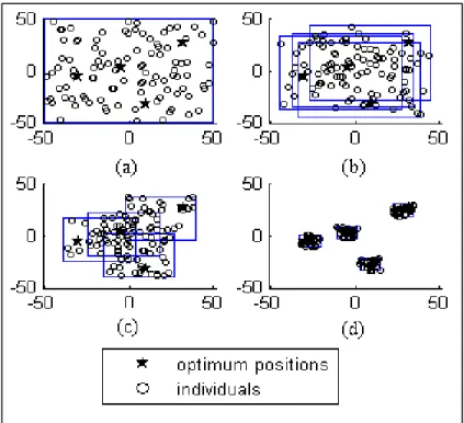
multi-site convergence processes (two and four optima) ...56 Figure 2.2 Representation of a uniformly random population with 100 individuals

bounded between [0, 1]2, where diversity is evaluated by: a) DL –

union of the area associated with each individual, b) DMST – total

length of the MST ...59 Figure 2.3 Diversity on P5 (solid curves) and P4 (dash curves) with respect to the

normalized location of x5 evaluated from: a) DPW, b) GFS, c) DL,

d) DMST ...63

Figure 2.4 Position of the optima for Cases 2 to 5 on: a) two-optima landscape, b) four-optima landscape ...65 Figure 3.1 Orthogonal EEB framework with differentiation into four search

zones ...75 Figure 3.2 Phenotypic diversity level of the new proposal registered over a

population of three individuals: a) Multiplicative formulation, b) Logarithmic formulation, c) Phenotypic convergence level of

PCM13 ...87

Figure 3.3 Fitness functions of the generic benchmark: a) Three translating cases of the linear landscape, b) Double-slope landscape and the saw tooth landscape ...90 Figure 3.4 PCM behavior observed over the linear landscape: a) PCM1,

b) PCM4.4 ...91

Figure 3.5 PCM behavior observed over the linear landscape: a) PCM5.1,

b) PCM10 ...93

Figure 3.6 PCM behavior observed over the linear landscape: a) PCM11,

b) PCM13 ...93

Figure 3.7 PCM behavior observed over the double-slope landscape: a) PCM4.3

(21)

Figure 3.8 PCM behavior observed over the double-slope landscape: a) PCM8,

b) PCM13 ...96

Figure 3.9 PCM behavior observed over the saw tooth landscape: a) PCM1 to

PCM8, b) PCM9 to PCM13 ...99

Figure 3.10 Sensitivity of PCM13 with respect to the population size (N) observed

over: a) Linear and double-slope landscapes, b) Saw tooth landscape ....102 Figure 3.11 Impact of outliers on PCM13 observed over the: a) Linear and

double-slope landscape, b) Saw tooth landscape ...103 Figure 3.12 Impact on PCM13 of outliers that are far away, observed over the

linear landscape: a) 1% outliers, b) 10% outliers ...104 Figure 3.13 Impact on PCM13 of outliers that are far away, observed over the

double-slope landscape: a) 1% outliers, b) 10% outliers ...104 Figure 3.14 Impact on PCM13 of outliers that are far away, observed over the

saw tooth landscape: a) 1% outliers, b) 10% outliers ...105 Figure 3.15 Impact of various selection plans over the EEB: a) 10D-F2,

b) 10D-F10 ...109 Figure 3.16 Impact of various replacement plans combined with FUSS selection

over the EEB: a) 10D-F2, b) 10D-F10...109 Figure 3.17 Impact of various population sizes over the EEB: a) 10D-F2,

b) 10D-F10 ...110 Figure 3.18 Impact of various crossover types over the EEB: a) 10D-F2,

b) 10D-F21 ...110 Figure 4.1 Diversity on P5 (solid curves) and P4 (dashed curves) with respect

to the normalized location of x5 evaluated from DLN ...117

Figure 4.2 Genotypic diversity levels of DNLN and DNPW for the unimodal

landscape ...119 Figure 4.3 Genotypic diversity level of DNLN (black curves) and DNPW

(gray curves) for a uniformly distributed population: a) Average diversity values over the complete process for three different multimodal structures, b) Average end diversity values for

multimodal structures ranging from 2 to 25 optima ...120 Figure 4.4 Genotypic diversity level of DNLN (black curves) and DNPW

(22)

monopolizing scheme: a) Average diversity values over the complete process for three different multimodal structures, b) Average end diversity values for multimodal structures ranging from 2 to 25

optima ...121 Figure 4.5 a) Effect of population size (N) on DNLN for the unimodal landscape,

b) Maximum difference among the four samplings over the unimodal landscape ...125 Figure 4.6 Effect of population size (N) on DN

PW for the unimodal landscape ...126

Figure 4.7 Effect of landscape dimensionality (n) on DNLN for the unimodal

landscape: a) with 1/n in the DNLN formulation, b) without 1/n in

the DNLN formulation ...127

Figure 4.8 Effect of landscape dimensionality (n) on DNLN for the multimodal

landscape (two optima): a) with 1/n in the DNLN formulation,

b) without 1/n in the DNLN formulation ...128

Figure 4.9 Maximum GDM value difference among the three samplings over the unimodal and multimodal (two optimum structure) landscapes: a) with 1/n in the DNLN formulation, b) without 1/n in the DNLN

formulation ...129 Figure 4.10 Effect of landscape dimensionality (n) on DNPW for: a) the unimodal

landscape, b) the multimodal landscape (two optima) ...130 Figure 4.11 Effect of outliers on DNLN for the unimodal landscape ...131

Figure 4.12 Effect of outliers on DNPW for the unimodal landscape ...132

Figure 4.13 Genotypic diversity level of DNLN and DNPW for the 10-D F2

function: a) Median run with 1 and 10 subpopulations, b) Mean of

the end diversity for different numbers of subpopulations ...135 Figure 4.14 Genotypic diversity level of DNLN and DNPW for the 10-D F8

the end diversity for different numbers of subpopulations ...136 Figure 4.15 Genotypic diversity level of DNLN and DNPW for the 10-D F10

the end diversity for different numbers of subpopulations ...137 Figure 5.1 General framework describing the adaptive process (steps in bold

type refer to fundamental components) ...145 Figure 5.2 Graphical model of BNGA ...154

(23)

Figure 5.3 Results of the hyperparameter sensitivity study: a) PM, b) AP ...165 Figure 5.4 Results of the hyperparameter sensitivity study: a) FAUC-RMAB,

(24)

(25)

LIST OF ALGORITHMS

Page Algorithm 1.1 GDMs benchmark ...27 Algorithm 1.2 Statistical procedure for GDMs sensitivity analysis ...39 Algorithm 4.1 Clustering RCGA search procedure ...133

(26)

(27)

LIST OF ABREVIATIONS

AP Adaptive Pursuit

AUC Area Under the Curve

BBOB Black-Box Optimization Benchmarking BGA Breeder Genetic Algorithm

BLX Blended crossover

BN Bayesian Network

BNGA Bayesian Network as Genetic Algorithms parameter adaptation approach CBR Case Base Reasoning

CEC Congress on Evolutionary Computation CMA Covariance Matrix Adaptation CPT Conditional Probability Table

DE Differential Evolution

DMAB Dynamic Multi-Armed Bandit DOE Design of Experiment

EA Evolutionary Algorithms

EDA Estimation of Distribution Algorithms EEB Exploration/Exploitation Balance

ES Evolution Strategies

FAUC Fitness-based Area Under the Curve FLC Fuzzy Logic Controller

FSR Fitness-based Sum of the Ranks FUSS Fitness Uniform Selection Scheme

(28)

GA Genetic Algorithms

GDM Genotypic Diversity Measure

GP Genetic Programming

KMP Klee Measure Problem

MA Memetic Algorithms

MAB Multi-Armed Bandit

MOOP Multi-Objective Optimization Problem NFL No Free Lunch theorem

PCM Phenotypic Convergence Measure

PCX Parent-Centric crossover

PDM Phenotypic Diversity Measure

PM Probability Matching

PNX Parent-centric Normal crossover PSO Particle Swarm Optimization RCGA Real-coded Genetic Algorithms RMAB Rank-based Multi-Armed Bandit RNG Random Number Generator

SLMAB Sliding Multi-Armed Bandit

SOM Self-Organizing Map

SR Sum of the Ranks

SSGA Steady-State Genetic Algorithms

(29)

(30)

(31)

LIST OF SYMBOLS

b Non uniform mutation parameter BEL( ) Posterior probability

BFE Best Fitness Error

C Scaling factor used by MAB approaches C Covariance matrix of the mutation distribution d(xi,xj) Distance function between individuals i and j

D( ) Diversity

D Distance-based diversity measure

D Decay factor used by RMAB

E Set of pairwise connections between individuals F Fitness distribution of a population

f Fitness

f Average fitness

G(X,E) Set of undirected Graph represented by X and E GF Gene Frequency diversity measure

H0 Statistical test null hypothesis

H/C ratio Number of hyperparameter required to control EA parameters J Total number of parameter states

l Length of the side of an hypercube S

LB Lower Bound

LD Length of the landscape Diagonal M Total number of intervals

MBFE Mean Best Fitness Error MST Minimum Spanning Tree n Landscape dimensionality and

Number of time a particular parameter state was selected

(32)

NMDF Normalization with Maximum Diversity so Far p Probability of a given SSGA parameter state p Fraction of N that belongs to an interval

pc Crossover probability

pm Mutation probability

P Population P(r|pi) Likelihood of pi given r

ˆq Empirical quality estimate

r Replacement plan

r Reward

roffspring Reward provided to SSGA parameters involved in offspring creation

rpopulation Reward provided to SSGA parameters involved in population governance

RWD Reward type

S(xi,l) Hypercube bounding the diversity contribution of individual i

SP Success Performance

SR Success Ratio

STD MBFE Standard Deviation

TC Total number of hyperparameters Combinations

u Minimum between M and N used for gene frequency normalization U( ) Uniform distribution

UB Upper Bound

V Volume of the landscape VMD Virtual Maximum Diversity

W Window size used by the reward schedule x Location of the individual on the landscape

ˆx Normalized location on the landscape

k

(33)

α Adaptation rate,

Normalization factor for Bayesian network inference, and Level of significance of a statistical test

β Learning rate

η PNX scattering parameter λ Number of created offspring

λr( ) Message pass from a child node to a parent node

μ Number of selected parents and Total length of the MST

μL Lebesgue measure

πr( ) Message pass from a parent node to a child node

σ Mutation step size

σε UNDX standard deviation parameter of a normal distribution

ση PCX and UNDX standard deviation parameter of a normal distribution

σζ PCX standard deviation parameter of a normal distribution

ˆ_f

σ Standard deviation of the fitness distribution

SUPERSCRIPT

N Normalized measure

t Generation number

* Argument for which the function reach the maximum value and Location of the global optimum

SUBSCRIPT

avg Average fitness of the individuals best Best individual in the population

(34)

i Individual number ∈ {1, 2, ..., N} and Identification number for SSGA parameter j Individual number ∈ {1, 2, ..., N} and

SSGA parameter state ∈ {1, 2, ..., J} k Gene locus ∈ {1, 2, ..., n}

m Interval number ∈ {1, 2, ..., M}

min Minimum probability for each parameter state

max Maximum probability that may reach a particular parameter state offspring Individual created by the generation plan

parent Individual picked from the selection plan s Selected state for a given parameter worst Worst individual in the population

(35)

INTRODUCTION

0.1 Background

Evolutionary algorithms (EA) are commonly used to optimize complex scientific problems. These methods attempt to emulate the theory of evolution through the survival of the fittest concept. Overall, the search process proceeds as follows: A population of N individuals is randomly generated, and then μ parents are selected from that population using strategies that promote fittest individuals. Subsequently, λ individuals, called offspring, are created by modifying the genotypic material of the parents. A number of operators can be used for this operation. They belong either to crossover or mutation operator, and, most of the time, they are activated following a probability pc and pm respectively. Then, some individuals from the

population are temporarily removed to make room for the offspring, and the empty places are filled by the set formed with the offspring and the removed individuals, following a defined update scheme. The evolution process is repeated until a predefined stopping criterion is met. Frequently, elite individuals are retained in subsequent generations to ensure that the best solutions found so far are not lost in the process.

EA offer many benefits, among them the ability to deal with discontinuous, multimodal, noisy, and high dimensionality landscapes, since no particular knowledge about the search space is required. They also face three major challenges:

1. They often converge prematurely over suboptimal solutions; 2. The evolution process is computationally expensive;

3. Their internal parameters are difficult to set.

These challenges have a direct impact on the performance achieved, as they weaken the robustness and efficiency of the EA search process. In other words, they can diminish the overall quality of the solutions found over a wide range of problems and extend the time required to locate them. As a matter of fact, achieving both robustness and efficiency is

(36)

rather difficult. This is demonstrated by the no free lunch (NFL) theorem, formulated by Wolpert and Macready (1997), which stipulates that, globally, no search algorithm dominates across all possible problems. This means that the selection of the most suitable optimizer is problem-dependent. In spite of the glaring conclusion of this result, the major research effort expended on these challenges is justified by the fact that practitioners are often interested in a specific class of problems, or they want to design search algorithms that have greater scope.

In terms of the first challenge, the stochastic nature of EA may help to alleviate the problem of premature convergence, since multiple search repetitions are prerequisite1. However, numerous modifications to the basic EA process have also been proposed over the years to address this problem. For instance, mechanisms for maintaining or promoting diversity inside a population constitute a broad class of mitigation responses (Sareni and Krähenbühl, 1998; Lozano, Herrera, and Cano, 2008; Das et al., 2011). Another important research theme related to premature convergence concerns the improvement of the EA search components. This approach includes the definition of smarter selection methods (Hutter and Legg, 2006), advanced variation operators (Kita, Ono, and Kobayashi, 1998; Deb, Anand, and Joshi, 2002; Beyer and Deb, 2001), and reformulation of the evolution model itself (Satoh, Yamamura, and Kobayashi, 1996). Other indirect alternatives might be beneficial, like assembling various optimizers into a portfolio, with the expectation of minimizing poor performance through the sharing of the computational budget (Peng et al., 2010).

With respect to the computational cost of EA processes, it is possible to attenuate its implications by leveraging the intrinsic population-based characteristic of EA, which allow parallel fitness evaluation of the individuals. Numerous models have been developed to achieve this, such as the master-slave framework and the multiple-deme approaches (Nowostawski and Poli, 1999; Alba and Troya, 2002; Konfrst, 2004; Munawar et al., 2008). Nevertheless, EA are often applied in simulation-based optimization problems, where evaluation of each individual may require a huge amount of computational time. Various

1_{From 30 to 100 repetitions are recommended (Wineberg and Christensen, 2007, p.3787), but, due to the computational burden}

(37)

strategies have been devised to overcome this problem, like the design of surrogate models for estimating the fitness function (Jin, 2005; Jin, Chen, and Simpson, 2001), or simply a prohibition mechanism for obviating the need to evaluate the same individuals multiple times (Corriveau, Guilbault, and Tahan, 2010).

Regarding the third challenge, more than ten parameters could be required from practitioners to carry out an EA process, from population size to the underlying operators of the evolution model. We believe that this is one of the motivations for the development of simplified metaheuristic variants, like differential evolution (DE) (Price, Storn, and Lampinen, 2005) and particle swarm optimization (PSO) (Kennedy, Eberhart, and Shi, 2001). Nonetheless, parameter setting has been a common theme of EA research since the inception of the field (Lobo, Lima, and Michalewicz, 2007). Consequently, many approaches have been developed in recent decades, and all of them can be considered to belong to one or other of the classes depicted in Figure 0.1 (Eiben, Hinterding, and Michalewicz, 1999).

Parameter tuning involves fixing parameters before the optimization process takes place. Practitioners could approach the procedure by applying their experience with similar problems, or by using more rigorous approaches, like design of experiments (DOE). In contrast, parameter control involves modifying the parameters during the course of the

(38)

evolution process. Deterministic parameter control usually relies on iteration-based rules, as no feedback is gathered from the search process. Conversely, in adaptive parameter control methods, the parameters are modified based on feedback from the search process. Finally, in self-adaptive parameter control methods, the parameters are directly encoded in the chromosome of the individuals. Methods in this last category are often considered as “evolution of the evolution”, since the EA process is responsible for modifying its own parameters.

Overall, this suggests that premature convergence, EA computational time, and parameter setting issues are intertwined. They are either a cause or an effect of the search path followed by the optimizer. In fact, parameter setting drives the direction of the search by regulating how resources are allocated. In contrast, premature convergence is a sign that the search path led to a dead end in terms of evolution, while excessive computational time may be evidence that the search path did not follow its optimal path. Consequently, we believe that addressing the parameter setting challenge might help prevent premature convergence, and it could also be the first rational step towards minimization of the search process computational time.

0.2 Research problem

In the previous section, we showed that resolving the parameter setting issue may help overcome the other EA challenges by guiding the search process towards its optimal path. However, this is a complex endeavor. In fact, EA parameters are problem-dependent, since particular parameter settings lead to specific algorithms to which the NFL theorem applies. Furthermore, parameter settings have been shown empirically to be evolution-dependent (Bäck, 1992; Stephens et al., 1998; Eiben, Hinterding, and Michalewicz, 1999; Yoon and Moon, 2002), and to interact in a number of ways (Odetayo, 1997; Darwen, 2000; Rojas et al., 2002; Nannen, Smit, and Eiben, 2008; Diaz-Gomez and Hougen, 2009).

The parameter setting categories identified in Figure 0.1 contain tuning approaches that can give us insight into the behavior of the parameters, and allow us, to some extent, to observe

(39)

the interactions among them. However, the results are valid only over a particular problem. Moreover, by itself, tuning is computationally intensive. In addition, it does not take into account the course of the evolution, because the parameters are set to be constant. In terms of deterministic control, generalization over different problems is troublesome, owing to the parameter setting schedule, which is user defined. Consequently, we believe that these approaches are not suitable responses to the challenges faced by EA.

In contrast, adaptive parameter control can be transferred from problem to problem. The course of its evolution is also taken into account through the information gathered from the search. Furthermore, nothing prevents adaptive control approaches from modeling the interaction among the parameters. However, in spite of these positive characteristics, there are major concerns with the adaptive system. For example, the relevance of the feedback indicator is crucial, and care must be taken to minimize its internal parameters, more commonly known as hyperparameters. As a matter of fact, it is useless to set EA parameters from a system requiring more hyperparameters, although exceptions would be possible if it could be demonstrated that the hyperparameters are far less sensitive than the EA parameters.

Self-adaptive control is attractive, as it is independent of the particular problem addressed. It also takes into account the evolutionary state, and the parameter interactions are implicitly handled. However, this comes at a price: increased dimensionality of the search space, and the process becoming a black box. Furthermore, parameters acting at the population level, like population size or selection method, require a special setting mechanism to aggregate the values proposed by the individuals (Eiben, Schut, de Wilde, 2006). Finally, in the words of Kramer (2010, p. 62), “evolution rewards short term success.” Therefore, parameter setting driven solely by the fitness of individuals, like self-adaptive control, can increase the occurrence of premature convergence.

Based on the above discussion, we believe that adaptive control is the most promising parameter setting scheme. However, as mentioned, an adaptation rule mechanism must be designed to enable all the parameters to be considered together and to involve as few

(40)

hyperparameters as possible. It must also have a proper feedback indicator. In order to investigate the applicability of the published adaptive approaches, we conducted a survey as part of this research, for which we collected and processed more than 100 papers on the topic. The outcomes of this survey are summarized in Figure 0.2.

The chart in Figure 0.2 illustrating the results of our survey shows that 88% of the adaptive parameter control proposals are restricted to two EA parameters or fewer, and no study was found in which more than four parameters were included. This suggests that no adaptive method can tackle all the EA parameters at once. In fact, most of the state-of-the-art adaptive systems are parameter independent (Goldberg, 1990; Thierens; 2005; Fialho, 2011). The lack of parameter interaction dependency makes difficult pursuing the optimal search path.

In terms of the feedback indicator, most of the studies proposing an adaptive mechanism endorse fitness improvement of the offspring. This is not surprising, given that the vast majority of adaptive control applications have been dedicated to setting the genetic operators and their related activation probabilities (see Figure 0.2). However, to expand the scope of

Figure 0.2 Survey of the published adaptive control approaches applied to EA parameter setting

(41)

the adaptive parameter setting process, the search path followed must be accounted for in some fashion.

One way to represent this feature is to measure the emphasis placed on exploration of the search space and exploitation of promising regions by the optimizer. This is a key characteristic which provides a means to interpret the way an algorithm works (Eiben and Schippers, 1998) and is commonly known as the exploration/exploitation balance (EEB). Too much exploration leads to prohibitive computational cost, while too much exploitation leads to premature convergence. Handling the EEB can be a great way to manage the other two EA challenges discussed in section 0.1 with respect to the parameter setting framework. However, Beyer (1998, p. 334) concluded his investigation of the subject by stating that there is no model in existence for conducting a deep evaluation of the relationship between EEB and EA performance. This observation was generalized by Eiben and Schippers (1998, p. 13), who maintain that there is no accepted reading of the EEB, and obviously intensive research is needed to better understand the essence of evolutionary search processes. In fact, exploration and exploitation are either regarded as opposing forces or orthogonal forces (Gupta, Smith, and Shalley, 2006). In the opposing forces framework, diminishing one aspect results in a proportional increase in the other. Conversely, in the orthogonal forces framework, it is possible to maximize both exploration and exploitation, as they are treated independently. Beyond this representational question, a means to assess exploration and exploitation is required.

Population diversity monitoring is the technique predominantly used for this assessment, although there is no consensus in the community about the best way to apply it. Either a genotypic formulation or a phenotypic formulation, or both, can be used (Olorunda and Engelbrecht 2008; Tirronen and Neri, 2009; Herrera and Lozano, 1996). The former is based on the location of the individuals over the search space, and the latter on the fitness distribution of the individuals. On top of that, numerous genotypic and phenotypic expressions have been proposed over the years; however, to the best of the authors’ knowledge, none was ever validated as a true population diversity metric.

(42)

Accordingly, we believe that developing an adaptive control system which supports all EA parameters while at the same time managing the search path through an appropriate feedback indicator remains an open challenge. Fialho emphasized the need for an advanced feedback indicator in the conclusion to his research on adaptive control parameter setting by declaring that (2011, p. 170) “[...] in order to efficiently tackle multi-modal problems, the maintenance of some level of diversity in the population should also be accounted somehow for [sic] in the rewarding of operator applications [...].”

0.3 Objective

That said, the objective of this thesis is to develop an adaptive parameter setting approach for controlling all the EA parameters at once. The work starts with the hypothesis that the search EEB, which serves as the feedback indicator, is most likely handled best by means of the orthogonal framework, where genotypic measurement is used to express the exploration axis, and phenotypic measurement is adopted to characterize the exploitation axis. To achieve the aim of this thesis, the following questions are investigated:

1. What is the best genotypic formulation for estimating the exploration provided by the search process?

2. What is the best phenotypic formulation for outlining the exploitation supplied by the search process?

3. How can the exploration and exploitation knowledge for adapting the EA parameters be converted into a reward?

4. Which adaptive system can best handle the parameter setting dependencies? 5. How can the performance of the adaptive parameter control proposal be assessed?

The core of this thesis is applied to real-coded genetic algorithms (RCGA) for continuous optimization problems. This does not limit the generality of the outcomes, however, as the concepts developed are directly applicable to any real-coded, population-based search process. It is to note also that the aim of this research is to bring flexible EA strategies, like

(43)

RCGA, to the performance level achieved by state-of-the-art EAs, like the covariance matrix adaptation evolution strategy (CMA-ES) (Hansen and Ostermeier, 1996).

0.4 Organization

To achieve the objective stated above, the thesis is divided into five chapters. The first four chapters relate to the assessment of the EEB concept through diversity measurements, while chapter 5 capitalizes on this knowledge with the development of an adaptive EA parameter control system. An overview of the topics covered and the relationships among them is illustrated in Figure 0.3.

In chapter 1, we review the genotypic diversity formulations that have been proposed over the years. From there, we develop a benchmark with various modalities for assessing the

(44)

behavior of these formulations. This study is performed using a controlled evolution process, in order to avoid any bias arising from a particular EA parameter setting system. The outcomes of the analysis enable us to identify similarities and differences in the genotypic formulations, as well as their limitations. This chapter provides the basis for answering question #1. The work described there was published in IEEE Transactions on Evolutionary Computation (Corriveau et al., 2012a).

In chapter 2, a more in-depth investigation of the genotypic diversity formulations is carried out by defining three requirements that must be met by a genotypic measurement in order to accurately estimate population diversity. Validation of these requirements is handled by a reduced population arrangement that we propose and seven cases of controlled population diversity. Four genotypic measures are specifically selected for this analysis. Elements of the response to question #1 are provided in this chapter, and the work described in it has been submitted to Applied Soft Computing for a forthcoming publication (Corriveau et al., 2012b).

In chapter 3, the study of chapters 1 and 2 is repeated, but this time from a phenotypic formulation standpoint. A review of the formulations considered is provided, along with their validation over the three diversity requirements reformulated within the phenotypic context. In addition, the results of this validation analysis are confirmed over a specifically designed benchmark, making it possible to observe the phenotypic formulation behavior over different fitness functions. A new phenotypic formulation is also proposed, and its performance is studied following the same approach. It is worth noting that the hypothesis supporting the usefulness of the phenotypic descriptor was justified in chapter 1 in a discussion about the most suitable EEB representation framework. Chapter 3 provides the answer to question #2. Furthermore, the outcomes of this investigation enable the introduction of an optimizer diagnostic tool dedicated to evaluating the impact of each parameter choice in terms of its EEB footprint. The value of such a monitoring tool lies in its ability to compare for instance, numerous common EA selection schemes, crossover operators, deletion schemes, and population sizes. This work has been published in the Applied Soft Computing journal (Corriveau et al., 2013).

(45)

Chapter 4 is devoted to evaluating a new genotypic diversity formulation introduced within the context of the EEB diagnostic tool presented in chapter 3. The analysis follows the same benchmark and validation framework that was defined in the first two chapters of this thesis, and completes our response to question #1.

In chapter 5, we fulfill the main objective of this thesis, which is the development of an adaptive parameter setting approach for controlling all the EA parameters at once. In order to achieve this, questions #3 to #5 are addressed. The proposed new system, which supports EEB management as the feedback indicator, takes advantage of the findings presented in the previous chapters. A flexible way to translate this knowledge into parameter rewards is also suggested. The key feature of our adaptive system is that all the EA parameters are handled and parameter interactions are supported. This is made possible by the use of a Bayesian network as the foundation for the adaptive control approach. The performance of this proposal is evaluated over a recognized benchmark (CEC’05) and compared with various state-of-the-art adaptive techniques, like G-CMA-ES. This work has been submitted for publication to the Applied Soft Computing journal (Corriveau et al., 2012c).

Finally, a summary of the results achieved is provided as conclusion. This is followed by recommendations for a future research effort towards the development of enhanced optimizers. Overall, the outcomes of this research are intended to provide practitioners with better optimization tools, although we do not claim, under any circumstances, that our approach is the best way to solve complex scientific problems.

(46)

(47)

CHAPTER 1

REVIEW AND STUDY OF GENOTYPIC DIVERSITY MEASURES FOR REAL-CODED REPRESENTATIONS

The exploration/exploitation balance (EEB) is a major concern in the control of evolutionary algorithms (EA) performance. Exploration is associated with the distribution of individuals on a landscape, and can be estimated by a genotypic diversity measure (GDM). In contrast, exploitation is related to individual responses, which can be described with a phenotypic diversity measure (PDM). Many diversity measures have been proposed in the literature without a comprehensive study of their differences. This chapter looks at surveys of GDMs published over the years for real-coded representations, and compares them based on a new benchmark, one that allows a better description of their behavior. The results demonstrate that none of the available GDMs is able to reflect the true diversity of all search processes. Nonetheless, the normalized pairwise diversity measurement (DNPW) proves to be the best

genotypic diversity measurement for standard EAs, as it shows non-dominated behavior with respect to the desired GDM requirements.

This chapter was published in IEEE Transactions on Evolutionary Computation (Corriveau et al., 2012a).

1.1 Introduction

One of the major problems with evolutionary algorithms (EA) is premature convergence (De Jong, 1975; Mauldin, 1984; Goldberg, 1989; Eshelman and Schaffer, 1991). However, no method exists that offers adequate control of this phenomenon. The origin of premature convergence is the exploration/exploitation balance (EEB) (Eiben and Schippers, 1998). Too much exploration leads to random searching and a waste of computational resources, while too much exploitation leads to local searching and premature convergence. This balance could be controlled by setting the EA parameters (Eiben, Hinterding, and Michalewicz,

(48)

1999). Here, we consider parameter-setting in the broad sense of the term. For example, the population number, the type of evolution model, and restart strategies are all possible options for controlling the EEB. It is worth noting that the EEB dilemma is not unique to EAs, as it is essentially a resource allocation problem that any adaptive system must face (Gupta, Smith, and Shalley, 2006; Ishii, Yoshida, and Yoshimoto, 2002; Lee and Ryu, 2002).

The EEB can be viewed conceptually following one of two paradigms. In one of these, exploration and exploitation can be regarded as opposing forces, which means that increasing one reduces the other, while in the other, they can be regarded as orthogonal forces (Gupta, Smith, and Shalley, 2006). This second paradigm offers the possibility of increasing both exploration and exploitation simultaneously.

In fact, the opposing forces paradigm is a special case of the orthogonal forces paradigm, in that, for a unimodal landscape, reducing exploration increases exploitation proportionally. However, the situation is different for a multimodal landscape, where exploration and exploitation can be intensified simultaneously. For instance, to locate each peak of a landscape having uniformly distributed peaks of the same amplitude, and a population size equal to the number of peaks, exploration and exploitation have to be maximized concurrently. With very rugged landscapes, exploration could be in a maximal state, but with poor exploitation. In contrast, if the population converges over a very rugged, restricted region, exploration and exploitation would be in a minimal state at the same time. Finally, a converged population over a small plateau would be characterized by poor exploration and extensive exploitation. From this we can conclude that the orthogonal EEB concept is more suitable than the opposing forces concept to represent any landscape type. It also demonstrates that it could be useful to consider both genotypic and phenotypic diversity to characterize a given landscape effectively.

Exploration is adequately monitored by genotypic diversity evaluation (diversity of solutions), whereas exploitation is better described by phenotypic diversity (diversity of solution responses). These two diversity measurements also refer to the quantity and quality

(49)

of the population diversity respectively (Herrera and Lozano, 1996). In fact, genotypic diversity is built from the spread of the individuals over the search space, and phenotypic diversity is defined by the fitness distribution of the population. This means that phenotypic diversity is synonymous with fitness diversity. With normalized evaluation, unitary genotypic and phenotypic diversity values relate to maximum exploration and exploitation respectively. It is important to note that, unlike genotypic diversity, phenotypic diversity defines maximum exploitation when it is in a state of convergence. Properly evaluating genotypic and phenotypic diversity is difficult, however. Multiple diversity measures have been proposed in the literature without a clearly elucidated study of their differences being performed. This chapter focuses on a comprehensive study of genotypic diversity measures (GDM).

Depending on the problem and the representation used, the number of diversity measures could be infinite (Burke, Gustafson, and Kendall, 2004). It is important, therefore, to clearly define the scope of applicability. First, the diversity measures considered here are those that can be related to the search space location of the individuals in the population. The diversity measures related to the tree structure representation, used in the genetic programming (GP) field, are not covered (Burke, Gustafson, and Kendall, 2004; McPhee and Hopper, 1999; Monsieurs and Flerackers, 2003). Also, the analysis is restricted to real-coded representations.

Diversity assessment is critical to monitoring and/or controlling the EEB. The aim of this chapter is to provide an initial stepping stone toward EEB management, and it does so by studying the similarities and differences among GDMs. Of course, a good GDM should be capable of representing the real genotypic diversity of a population. However, it should also:

1. Demonstrate repeatability with respect to a similarly scattered population;

2. Be robust with respect to the simulation parameters, like population size and landscape dimensionality;

(50)

To perform this comparison task, our complete analysis makes use of a new, simple benchmark that allows clear definition of the tested indicator behavior. Furthermore, we restricted this study to the available GDM formulations provided in the literature. The chapter is organized as follows: the next section, section 1.2, describes the various genotypic diversity measures studied; section 1.3 presents the published comparative studies; section 1.4 discusses the proposed benchmark; section 1.5 presents the results; section 1.6 validates the use of the proposed benchmark; and section 1.7 provides our concluding discussion.

1.2 Genotypic diversity measure

Even though no consensus has emerged on the definition of diversity (Lieberson, 1969; Patil and Taillie, 1982), the concept can be defined as the degree of heterogeneity or homogeneity between individuals in a studied population (Gouvêa Jr. and Araújo, 2008).

1.2.1 General concept

Genotypic diversity can be evaluated using one of two approaches. The first is based on a measurement of the distance between individuals. This distance may be evaluated from the mean spatial position of the population (Ursem, 2002; Abbass and Deb, 2003; Morrison and De Jong, 2002), from the position of the fittest individual (Herrera and Lozano, 1996), or the position of each of the individuals, which in this case would range from the pairwise measure (Olorunda and Engelbrecht, 2008; Barker and Martin, 2000) to the maximum distance between two individuals (Olorunda and Engelbrecht, 2008). The Euclidian distance is more common for distance estimation with real-coded genes, since the landscape is defined in a Euclidian space Rn, where n represents the landscape dimensionality.

The second approach scans gene frequency. This concept is generalized from binary representations, where the probability of the alleles at each locus is calculated within the complete population (Wineberg and Oppacher, 2003). In a real-coded framework, all genes are continuous. Consequently, gene scanning requires gene partitioning. The predefined

(51)

intervals (m ∈ {1, 2, ..., M}) are then considered as possible alleles. Ichikawa and Ishii (1993) applied this procedure to integer representations, and the technique was later generalized to any symbolic alphabet by Wineberg and Oppacher (2003). Nevertheless, the number of intervals (M) involved in the discretization constitutes a severe limitation; they directly influence diversity estimation, which could make it difficult to achieve meaningful usage for a small population size or high dimensionality. Moreover, the gene frequency combination among all landscape variables must be defined. For example, Gouvêa Jr. and Araújo (2008) proposed using a representative gene to characterize the population diversity. In other words, the diversity measure is reduced to the consideration of only one gene or landscape variable characterizing the individuals. As they mentioned, the selected gene has to be a significant one. Therefore, to avoid a misleading diversity estimation, an average evaluation obtained from the diversity measure of each gene may be preferred (Wineberg and Oppacher, 2003). Collins and Jefferson (1991) also used the average gene frequency to determine the population diversity. However, this study was limited to binary representations.

1.2.2 Normalization

Normalization of the various GDMs is preferable for comparison purposes, as the descriptors can then be evaluated on the same basis.

When defined, the maximum value can be used as a normalization factor. In the case of distance measurement, the landscape diagonal (LD), that is, the maximum distance between opposite corners of the landscape, can also be used for normalization. Otherwise, the following simple normalization approach is proposed: the maximum value obtained so far during the evolution process of a given problem could serve as a normalization factor. The first iteration then becomes the reference, until a more diverse population is found. Since the initial EA population is generally created from a random uniform distribution, it is supposed to be the most diverse population. However, as information continues to arrive during the process, the indicator is updated if required. This normalization method is referred to here as

(52)

NMDF (Normalized with Maximum Diversity so Far). NMDF is similar to the normalization used by Herrera et al. (1994).

1.2.3 Genotypic diversity measures

The GDMs based on distance measurements (D) and gene frequency (GF) considered in this chapter are listed in the following table. They are presented in their normalized form. The asterisk following specific equation indicates that the corresponding measure uses a normalization method not defined in its original form.

The 1st GDM in this table corresponds to the diameter of the population (DNDP), which is a

pairwise measure considering only the distance between the two most widely separated individuals in the population.

The 2nd GDM (Olorunda and Engelbrecht, 2008) represents the radius of the population (DNRP), and determines the distance between the individual farthest away and the mean

position of the population. It is possible to generalize DRP to account for only a certain

fraction (f) of the individuals around the mean position. This leads to the 3rd GDM in Table 1.1, DNRP (f), where the population size is sorted in ascending order with respect to the mean

position. Therefore, extreme individuals can be set aside.

The 4th GDM, proposed by Ursem (2002), is the distance-to-average-point measure (DNDTAP), and it represents the mean radius of the population. In this study, a modified

normalization version of this GDM is also considered, that is, DN2DTAP, which is presented as

the 5th GDM in Table 1.1. With this form, the LD normalization factor is replaced by NMDF. This expression can also be considered as the normalization alternative to the DDTAP

measure proposed by Abbass and Deb (2003). No justification was provided in (Ursem, 2002; Abbass and Deb, 2003) to justify the usefulness of DDTAP, except its intuitive

(53)