Object detecion in static image /application to animal detectiom

(1)

Ministry of High Education and Scientific Research

ــــــــــــــــ

ـ

ــــــــــــــــــــــــــــــــــــــــــــــــــــــــــــــــــــــــــــــــــ

Echahid Hamma Lakhder University EL-OUED Faculty of Science Exact

Department of computer science

Graduation Memory

ACADEMIC MASTER

Department : Mathematics and Computer Science

Section : Computer Science

Specialty: Distributed Systems and Artificial Intelligence

Theme

Presented by: GORI Abdessamad

HAMIDANI Djabari

Mr. KHABACH Mohib Eddine MAA Univ. Eloued Rapporter Mr. ZAIZ Fouzi MAA Univ. Eloued President Miss GUETTAS Chourouk MAA Univ. Eloued Examiner

Academic year 2017/2018 .

Object detection in static image :

application to animal detection

(2)

Computer vision is one of the most important fields of artificial intelligence designed to build intelligent applications that are capable of understanding the content of images as understood by humans. Among these applications is detection of in images. One of the most difficult situations is recognizing and locating animals. Because it does not have a specific shape or a fixed position with the change of lighting. In this study we have collected the most important algorithms (HOG,LBP) related to the extraction of properties of objects from images, and used the most important classifiers(SVM,RF)in machine learning, and try to solve the previous problems.

Key words : Computer Vision, Artificiel Intelligence, Object detection, Machine learning, HOG,LBP,SVM,RF, Image treatment.

:صخلملا

لا تلااجم مها نم ةيبوساحلا ةيؤرلا دعت ذ يعانطصلاا ءاك فدهت ىلإ ءانب تاقيبطت ةيكذ ةرداق ىلع مهف ىوتحم روصلا امك اهمهفي ناسنلإا ه نيب نمو , دحا .ةروصلا يف هعقوم ديدحتو نئاكلا فشك تاقيبطتلا هذ ريغت عم ةتباث ةيعضو وا ددحم لكش لمحت لا ةريخلاا هذه اهنلا .تاناويحلا ديدحتو فرعتلا يه تلااحلا بعصا تايمزروخلا مها عمجب انمق ةساردلا هذه يف .ةءاضلاا ةلاح (HOG,LBP) صئاصخ جارختساب ةقلعتملا وصلا نم تانئاكلا تافنصملا مها انلمعتساو ر (SVM,RF) ةدوجوملا يف لذو ةللاا ملعت لحل انم ةلواحم ك .تاناويحلا ديدحت لكاشم ,ةيبوساح ةيؤر ,يعانطصا ءاكذلا ,ةللاا ملعت : ةيحاتفملا تاملك HOG , LBP,SVM,RF ,ءايشلاا ديدحت, روصلا ةجلاعم يئاقتنلاا ثحبلا,ةقلزنملا ةذفانلا, .

Résume:

La vision par ordinateur est l’un des domaines les plus importants de l’intelligence artificielle, conçu pour créer des applications intelligentes capables de comprendre le contenu des images telles qu’elles sont comprises par les humains. Parmi ces applications, on trouve la détection de l'objet et son positionnement dans l'image ou la vidéo. L'une des situations les plus difficiles est l'identification et l'identification des animaux. Parce qu'il n'a pas de forme spécifique ou de position fixe avec le changement d'éclairage. Dans cette étude, nous avons recueilli les algorithmes les plus importants liés à l'extraction des propriétés des objets à partir d'images et utilisé les travaux les plus importants pour apprendre la machine et essayer de résoudre les problèmes précédents.

(3)

General Introduction………..

1

16

4.2.1 Sliding windows……….

16

4.2.2 Selective search………...

17

5. Conclusion………..

17

Chapter II : Related Works

1. Introduction ………...

19

2.Animal Detection………

19

2.1 Related Works………

19

2.2 Challenges and issues……….

21

2.2.1 Animal body vs. animal face………..

22

(4)

32

2.2.1.2 Algorithm selective search………..

32

2.2.2 Avoid false positive……….

33

2.2.2.1 Non maximum suppression………. 33

2.2.2.2 Heat map……….. 34

3. The equipment used for system………..

34 3.1 Platform Anaconda………. 35

3.2 Python ……….. 37

3.3 OpenCV………. 37

4. Conclusion ……….

38 Chapter IV : Experiment and result

1. Introduction………

40 2. Implementation………...

40 2.1 Training……….. 40

2.2 Detection……… 41

2.2.1 Detectors experiment……….. 42

2.2.2 Performance evaluation………... 47

3. Perspective………... 49

4. Conclusion……… 49

General Conclusion……….. 50

(5)

Figure 1.1 Image Classifiction………. 6

Figure 1.2.Object Detection………. 7

Figure 1.3. Image recognition pipeline……… 9

Figure 1.4 .hog………. 11

Figure 1.5. Random Forest……….. 16

Figure 1.6. Image pyramid………

17 Figure 2.1.Various body postures……… 22

Figure2.2.Light conditions………... 23

Figure 2.3.Accuracy of detection………. 23

Figure 2.4.Image samples……… 24

Figure3.1 System Architecture………. 28

Figure 3.1.Positive Database……… 29

Figure3.3.Negative Database………... 29

Figure 3.4.NMS Algorithm……….. 34

Figure 3.5.Heat map………. 34

Figure 3.6 .Anaconda Navigator……….. 36

Figure 4.1 Relationship between detection rate and the number

positive training database

41 Figure 4.2 Exprimental images……… 42

Figure 4.3 Relationship between nombre regions and algorithm

detection

43 Figure 4.4 SW+SVM+HOG………... 43

Figure 4.5 SW+SVM+LBP……….. 44

Figure 4.6 SW+RF+HOG……… 44

Figure 4.7 SW+RF+LBP………. 44

Figure 4.8 SS+SVM+HOG………. 45

Figure 4.9 SS+SVM+LBP………. 45

Figure 4.10 SS+RF+HOG………... 45

Figure 4.11 SS+RF+LBP……… 46

Figure 4.12 Relationship between detectors and false positive of

sliding window

46 Figure 4.13 Relationship between detectors and false positive of

sliding window

(6)

(7)

Table2.1 Overview………... 21

Table 4.1 Trained model………... 40

Table 4.2 Detectors list………. 41

Table

4.3 Test results……… 42

(8)

1 | P a g e

General Introduction

Vision is one of the most powerfull that humans had gifted. That powerfull ability we as human were trying to understand it so we can develop it and heal it an exploit it much more. While trying to understand that ability we known how much powerfull it is, so we jumped to the next step which is given it to the machines that we made.

Today researches about the vision of the machines or as we should call it computer vision are huge and tremendous. We managed to make smart computers and machines. But yet blind, so many solutuions today were proposed but none was enough even with the enormous and huge technological development. There are some performing solutions but in each there is always a lacking; whether its their high price or their poor adaptability. The problem we want to solve is animal detection.

Our objective is to provide an easy using system that, can help keep the roads safer. Yet with protecting animals in the roads, that leads us to ask some questions for the study like, how the system will make the process easier, how the system will make the roads safer and how to protect animals.

The importance of this study resides in prevention of animal- vehicle accidents and will increase human and wildlife safety, it will detect large animals before they enter the road and warn the driver also helps in saving crops in farm from animals.

Researches related to animal’s detection in image processing have been an important aspect to numerous applications. Many algorithms and methods have been developed by human being related this. Intelligent video surveillance systems deal with the real-time

monitoring of persistent and transient objects within a specific environment. The primary aim of this system is to test and compare between different type of algorithm and methods to produce an effective system with fast detection time and better accuracy detection.

Other works similar to our system failed to do an effective automated system and some failed to make a cheap system. Others failed to make a real time detection system.

This report will contains four chapters :

(9)

2 | P a g e Chapter 2 : Will contain other similar works and their evaluation, with Challenges and issues of our study.

Chapter 3 : Contains the architecture of the system and our system phases and algorithmes Chapter 4 : The last chapter will be about the implementation of the system and the

obtained results and our perspectives. Finally the general conclusion.

(10)

Chapter 1

Background and motivation

(11)

3 | P a g e

1. Introduction

One of the important fields of Artificial Intelligence(AI) is Computer Vision. Computer Vision is the science of computers and software systems that can recognize and understand images and scenes . The success of that field was enabled because of the emerge of another huge field of AI which is Machine Learning.

Machine learning uses statistical techniques to give computer systems the ability to "learn", without being explicitly programmed.

Computer Vision is also composed of various aspects such as image recognition, object detection, image generation, image super-resolution and more. Object detection is probably the most profound aspect of computer vision due the number practical use cases. Hence, object detection is typically viewed as a machine learning pattern recognition problem where the goal is to given an image to classify it as an object or non-object.

In this chapter we will be defining the main elements and notions in our project along with the definition of our problem and the represented solutions in today‟s reality, trying to realize a new perception using what the technology is offering.

2. Computer vision

The goal of computer vision is to make useful decisions about real physical objects and scenes based on sensed images. In order to make decisions about real objects, it is almost always necessary to construct some description or model of them from the image. Because of this, many experts will say that the goal of computer vision is the construction of scene description from images [1].

Computer vision is closely linked with artificial intelligence, as the computer must interpret what it sees, and then perform appropriate analysis or act accordingly.

(12)

4 | P a g e Computer Vision is an emulation of human vision using digital images through three main processing components, executed one after the other[2]:

2.1 Image acquisition

:

The general aim of Image Acquisition is to transform an optical image (Real World Data) in to an array of numerical data which could be later manipulated on a computer, before any video or image processing can commence an image must be captured by camera and converted into a manageable entity. The Image Acquisition process consists of three steps [3]:

 Optical system which focuses the energy  Energy reflected from the object of interest  A sensor which measure the amount of energy

2.2 Image processing

:

The second component of Computer Vision is the low-level processing of images. Algorithms are applied to the binary data acquired in the first step to infer low-level information on parts of the image. This type of information is characterized by image edges, point features or segments, for example. They are all the basic geometric elements that build objects in images.This second step usually involves advanced applied mathematics algorithms and techniques [3].

2.3 Image analysis

The last step of the Computer Vision pipeline if the actual analysis of the data, which will allow the decision making. High-level algorithms are applied, using both the image data and the low-level information computed in previous steps [3][2].

Examples of high-level image analysis are: 1. 3D scene mapping

2. Image recognition 3. Object tracking

(13)

5 | P a g e

2.3.1 Image recognition :

Image recognition, in the context of machine vision, is the ability of software to identify objects, places, people, writing and actions in images. Computers can use machine vision technologies in combination with a camera and artificial intelligence software to achieve image recognition.

Image recognition is used to perform a large number of machine-based visual tasks, such as labeling the content of images with meta-tags, performing image content search and guiding autonomous robots, self-driving cars and accident avoidance systems.

While human and animal brains recognize objects with ease, computers have difficulty with the task. Software for image recognition requires machine learning [4].

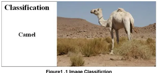
2.3.2 Image classification :

Classification is the process of categorizing a stimuli into a finite set of classes or labels. The process normally involves recognition of the dominant content in a scene.

Classification involves invariant recognition of the image content. In simple terms classification is concerned about what is in the scene and not where it is.figure1.1

(14)

6 | P a g e

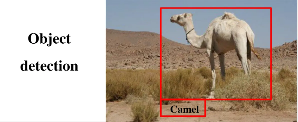
2.3.3 Object detection

The object recognition problem can be defined as a labeling problem based on models of known objects. Formally, given an image containing one or more objects of interest (and background) and a set of labels corresponding to a set of models known to the system, the system should assign correct labels to regions, or a set of regions, in the image [4].

All object recognition systems use models either explicitly or implicitly and employ feature detectors based on these object models. The hypothesis formation and verification components vary in their importance in different approaches to object recognition. Some systems use only hypothesis formation and then select the object with highest likelihood as the correct object [4]. Figure1.2

detection=classification + localization

An object detection system is tasked to categorize and locate all known content in the scene.[4]

Figure 1.2.Object Detection

3. Machine learning :

Machine learning is a subfield of artificial intelligence (AI). The goal of machine learning generally is to understand the structure of data and fit that data into models that can be understood and utilized by people [5].

It differs from traditional computational approaches. In traditional computing An algorithm is a sequence of instructions that should be carried out to transform the input to output.

Object

detection

(15)

7 | P a g e Machine learning is not just a database problem; it is also a part of artificial intelligence. To be intelligent, a system that is in a changing environment should have the ability to learn. If the system can learn and adapt to such changes, the system designer need not foresee and provide solutions for all possible situations [7].

Machine learning is programming computers to optimize a performance criterion using example data or past experience. We have a model defined up to some parameters, and learning is the execution of a computer program to optimize the parameters of the model using the training data or past experience. The model may be predictive to make predictions in the future, or descriptive to gain knowledge from data, or both [5].

Machine learning also helps us find solutions to many problems in vision, speech recognition, and robotics [5].

3.1

Supervised learning :

Supervised learning is based on training a data sample from data source with correct classification already assigned [6].

Supervised learning is the machine learning task of learning a f unction that maps an input to an output based on example input-output pairs [8].

It infers a function from labeled training data consisting of a set of training examples Supervised learning divide into [7]:

3.1.1 Classification :

A classification problem is when the output variable is a category, such as "red" or "blue" or "disease" and "no disease".

3.1.2 Regression :

A regression problem is when the output variable is a real value, such as "dollars" or "weight" [9].

3.2

Unsupervised Learning :

Is to learn using unsupervised learning algorithm. This unsupervised refers to the ability to learn and organize information without providing an error signal to evaluate the potential

(16)

8 | P a g e solution. The lack of direction for the learning algorithm in unsupervised learning can sometime be advantageous, since it lets the algorithm to look back for patterns that have not been previously considered [6].

Unsupervised learning divide into :

3.2.1 Clustering :

A clustering problem is where you want to discover the inherent groupings in the data, such as grouping customers by purchasing behavior .

3.2.2 Association :

An association rule learning problem is where you want to discover rules that describe large portions of your data, such as people that buy X also tend to buy Y [9].

4 Object recognition and object detection :

An object recognition or as some call it image recognition or sometimes you can find it as images classification. An object recognition identifies which objects are present in an image. It takes the entire image as an input and outputs class labels and class probabilities of objects present in that image.

On the other hand, an object detection algorithm not only tells you which objects are present in the image, it also outputs bounding boxes (x, y, width, height) to indicate the location of the objects inside the image.

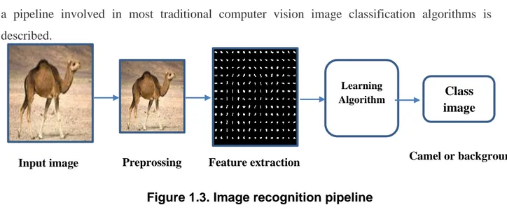
4.1

Image recognition pipeline :

Image recognition algorithms go through some steps which are represented in a pipeline, a pipeline involved in most traditional computer vision image classification algorithms is described. Learning Algorithm Class image Feature extraction Preprossing Input image Camel or background

(17)

01 | P a g e

4.1.1 Preprocessing :

Often an input image is pre-processed to normalize contrast and brightness effects. A very common preprocessing step is to subtract the mean of image intensities and divide by the standard deviation.

As part of pre-processing, an input image or patch of an image is also cropped and resized to a fixed size. This is essential because the next step, feature extraction, is performed on a fixed sized image.

4.1.2 Feature extraction :

Features are functions of the original measurement variables that are useful for classification and/or pattern recognition. Features extraction is the process of defining a set of features, or image characteristics, which will most efficiently or meaningfully represent the information that is important for detection analysis and classification [9]. The purpose of features extraction is to enhance the effectiveness and efficiency of object detection and classification.

Many feature extraction methods focus on object detection and recognition. We will discuss two different types of simple features (or descriptions),which are HOG (Histogram of Oriented Gradient) and LBP (Local binary patterns). All of the two popular features are widely used in object detection or target tracking like human-face (eyes), pedestrian, traffic signs, character recognition, animals in roads ,etc.

4.1.2.1 Histogram of Oriented Gradients :

Histogram of Oriented Gradients (HOG) are another popular image descriptors used in image processing for the purpose of target detection. It is proposed by Dalal and Triggs who focused their algorithm on the problem of pedestrian detection, and had an excellent performance compared with other feature sets. The advantage of HOG descriptor is that it can describe contour and edge feature outstandingly in objects other than human beings, such as bicycles, and cars, as well as common animals such as dogs, camel [10].

(18)

00 | P a g e

Figure 1.4 .hog

Gradient computation :

Before the computation of the gradient values, gamma/color normalization would be applied to improve the performance . After that, the gradient direction and gradient magnitude of each pixel would be calculated [10]. The horizontal and vertical gradient obtained by convolution the simple but best 1-D gradient operator:

horizontal operator:[−1, 0, 1] ,ˆ vertical operator:[−1, 0, 1]T which means, the gradient of pixel (x, y) is:

where, Gx(x, y) and Gy(x, y) are the horizontal gradient and vertical gradient of point (x, y) respectively, H(x, y) is the pixel gray value. Then, the gradient magnitude G(x, y) and gradient direction α(x, y) can be obtained as :

Input image

Gamma & Color normalization

Gradient computation Block & cell

divition

(19)

01 | P a g e

Cell histograms and HOG feature vector generation :

The next step after gradient computation is to create the cell histograms. The image window was divided into several larger spatial regions called “blocks” which contain small spatial regions called “cells”, for each cell accumulating a local 1-d histogram of gradient directions voted by the pixel‟s gradient direction and magnitude in this cell. To calculate the final feature vector for the entire image .

Assume there are N blocks in a image window and each block contains 4 cells divided into 9 bins , The bins of the histogram correspond to gradients directions 0, 20, 40 … 160 degrees . the final HOG feature vectors should be N × 4 × 9 = 36N dimensions. After we extract the HOG feature vectors, a classification algorithm would be applied to detect the target.

4.1.2.2 Local Binary Patterns (LBP) features :

Local Binary Patterns (LBP) introduced as another powerful local descriptor for microstructures of images in computer vision . In general, it is an efficient image feature which transforms an image into an array or image of integer labels describing small scale appearances of the images. These labels or statistic histogram, are then applied for further image analysis. Currently, LBP feature is widely used in texture analysis, target detecting and tracking, face recognition analysis, product quality analysis, surface inspection, etc [11].

Concept :

The LBP feature vector, in its simplest form, is created in the following manner [11]:  Divide the examined window into cells (e.g. 16x16 pixels for each cell).

 For each pixel in a cell, compare the pixel to each of its 8 neighbors (on its top, left-middle, left-bottom, right-top, etc.). Follow the pixels along a circle, i.e. clockwise or counter-clockwise.

 Where the center pixel's value is greater than the neighbor's value, write "0". Otherwise, write "1". This gives an 8-digit binary number (which is usually converted to decimal for convenience).

(20)

02 | P a g e  Compute the histogram, over the cell, of the frequency of each "number" occurring (i.e.,

each combination of which pixels are smaller and which are greater than the center). This histogram can be seen as a 256-dimensional feature vector.

 Optionally normalize the histogram.

 Concatenate (normalized) histograms of all cells. This gives a feature vector for the entire window.

4.1.3 Learning Algorithm For Classification :

In the previous section, we learned how to convert an image to a feature vector. In this section, we will learn how a classification algorithm takes this feature vector as input and outputs a class label ( e.g. camel or background ).

Before a classification algorithm can do its magic, we need to train it by showing thousands of examples of cats and backgrounds. Different learning algorithms learn differently, but the general principle is that learning algorithms treat feature vectors as points in higher dimensional space. Now let us look at some learning algorithms that we are going to use in this thesis, Support Vector Machines ( SVM ) and Random Forest.

4.1.3.1 Support Vector Machines ( SVM ) :

Support Vector Machines (SVM), also called Support Vector Networks, is another famous and powerful pattern recognition classification algorithm improved by Vapnik . SVM has a very wide range of applications in data analysis, regression analysis, pattern recognition, etc. We only focus on its application in image classification and image recognition tasks. A classical application in SVM is pedestrian detection proposed by Navneet Dalal and Bill Triggs. Some improved application based on SVM in traffic sign classification and people & vehicle detection and other objective detection shown SVM has an outstanding ability in image recognition and classification. support vector machine (SVM) is a computer algorithm that learns by example to assign labels to objects [6].

In essence, an SVM is a mathematical entity, an algorithm (or recipe) for maximizing a particular mathematical function with respect to a given collection of data. The basic ideas behind the SVM algorithm, however, can be explained without ever reading an equation.

(21)

03 | P a g e Indeed, to understand the essence of SVM classification, one needs only to grasp four basic concepts: (i) the separating hyperplane, (ii) the maximum-margin hyperplane, (iii) the soft margin (iv) the kernel function.

i. Separating hyperplane :

The separating hyperplane is a line that separates the profile into clusters.

ii. The maximum-margin hyperplane :

The concept of treating the objects to be classified as points in a high-dimensional space and finding a line that separates them is not unique to the SVM. The SVM, however, is different from other hyperplane-based classifiers by virtue of how the hyperplane is selected.

We have now established that the goal of the SVM is to identify a line that separates profiles in this two-dimensional space. However, many such lines exist. Which one provides the best classifier?

If we define the distance from the separating hyperplane to the nearest expression vector as the margin of the hyperplane, then the SVM selects the maximum margin separating hyperplane. Selecting this particular hyperplane maximizes the SVM‟s ability to predict the correct classification.

iii. The soft margin :

we have assumed that the data can be separated using a straight line. Of course, many real data sets cannot be separated as cleanly instead, where the data set in real world contains „error‟, Intuitively, we would like the SVM to be able to deal with errors in the data by allowing a few anomalous expression profiles to fall on the „wrong side‟ of the separating hyperplane. To handle cases like these, the SVM algorithm has to be modified by adding a „soft margin‟ Essentially, this allows some data points to push their way through the margin of the separating hyperplane without affecting the final result.

iv. The kernel function :

It computes the similarity of two data points in the feature space using dot product. • The selection of an appropriate kernel function is important, since the kernel function defines the feature space in which the training set examples will be classified.

• The kernel expresses prior knowledge about the phenomenon being modeled, encoded as a similarity measure between two vectors.

(22)

04 | P a g e • A support vector machine can locate a separating hyperplane in the feature space and classify points in that space without even representing the space explicitly, simply by defining a kernel function, that plays the role of the dot product in the feature space [9].

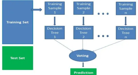
4.1.3.2 Random Forest :

Random forests, like decision trees, can be used to solve classification and regression problems but it is able to overcome the drawbacks associated with single decision trees while maintaining the benefits. The random forests model calculates a response variable (e.g., land cover, percent tree cover) by creating many (usually several hundred) different decision trees (the forest of trees) and then putting each object to be modeled (in our case the object is a multi-layered pixel) down each of the decision trees. The response is then determined by evaluating the responses from all of the trees. In the case of classification the class that is predicted most is the class that is assigned for that object (Leo Breiman & Cutler A.) [11]. In other words, if 500 trees are grown and 400 of them predict that a particular pixel is forest and 100 predict it is grass the predicted output for that pixel will be forest. In the case of regression the resulting value for an object is the mean of all of the predictions. Since predictions from random forests are derived using a forest of trees it is not possible to easily illustrate how the predictions are made.

It works in four steps:

1. Select random samples from a given dataset.

2. Construct a decision tree for each sample and get a prediction result from each decision tree.

3. Perform a vote for each predicted result.

(23)

05 | P a g e

4.2 Object detection

:

At the heart of all object detection algorithms is an object recognition algorithm. Suppose we trained an object recognition model which identifies camels in image patches. This model will tell whether an image has a camel in it or not. It does not tell where the object is located.

To localize the object, we have to select sub-regions (patches) of the image and then apply the object recognition algorithm to these image patches. The location of the objects is given by the location of the image patches where the class probability returned by the object recognition algorithm is high.

Sliding window and selective search These techniques give us all the possible location in input the image.

4.2.1 Sliding windows :

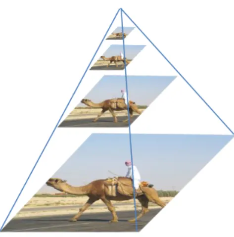
In the sliding window approach, we slide a box or window over an image to select a patch and classify each image patch covered by the window using the object recognition model. It is an exhaustive search for objects over the entire image. Not only do we need to search all possible locations in the image, we have to search at different scales (image pyramid) . This is because object recognition models are generally trained at a specific scale (or range of scales). This results into classifying tens of thousands of image patches.

(24)

06 | P a g e image pyramid is created by scaling the image. Idea is that we resize the image at multiple scales and we count on the fact that our chosen window size will completely contain the object in one of these resized images.

4.2.2 Selective search :

Selective Search is a region proposal algorithm used in object detection. It is designed to be fast with a very high recall. It is based on computing hierarchical grouping of similar regions based on color, texture, size and shape compatibility.

Selective Search starts by over-segmenting the image based on intensity of the pixels using a graph-based segmentation method by Felzenszwalb and Huttenlocher [12]. Selective Search algorithm takes these over segments as initial input and performs the following steps :

1. Add all bounding boxes corresponding to segmented parts to the list of regional proposals 2. Group adjacent segments based on similarity

3. Go to step 1

5 Conclusion

In this chapter we had defined the main elements and concepts involved in this projects. Trying to clarify and offer a background, by discussing the different technologies involved. Problems we talked about are just a piece of the big picture, but we did focus on the important ones. Many solutions and systems were provided either manual or automated, but each still miss something.Next chapter we will provide a better look into existing systems. Going through they‟re architectures and how they works, depending on the criteria points.

(25)

Chapter 2

Related Works

(26)

91 | P a g e

1. Introduction

The existing of an animal detection system is necessary. Because of, firstly, the roads accidents, also protecting the animals lives. Secondly, make the life safer and easier. Also have safer roads and secure rare desert animals that can be killed every day in roads. Finally

exploiting the technology to provide for better purpose.

In this chapter we will discuss some related works, trying to demonstrate the points that others failed to cover and the strong points in those systems. Showing the differences between those systems, and what will our system include eventually.

2. Animal Detection :

A natural way to detect animals using cameras is through one of the existing detection schemes, especially those applied for pedestrian detection such as detection through texture features, color features or gradient features (which are robust to illumination changes and hence more applicable to nighttime conditions). Unfortunately, directly applying one of these schemes, developed initially to detect other object such as pedestrian or TS, has apparent difficulties. This is due to the fact that animals have their specific properties including height, shape, texture and different views (rear-view, front view and side-view), which distinguish them from other objects, such as pedestrian. That is, an adaptation of the current detection schemes is mandatory.

In this section we review some schemes related to the detection and recognition of animal in, which might help to design animal detection and recognition schemes. We focus only on algorithms applied on large animal.

2-1 Related Works :

Table 2.1 gives the summary of active animal detection system based on image processing technology.

(27)

02 | P a g e

Year

Reference

Technique

Advantages

Disadvantage

2006 Tilo Burghardt and Janko Calic. Real-time face detection and tracking of animals [12] 1 Haar-like features based on AdaBoost and image feature based tracking -Real-time 2 -Smooth and accurate -tracking included

-Some false positive -Only focus on face detection 2009 Chen Peijiang. Moving object detection based on background extraction [13] Background subtraction method after getting the background image -Very fast 3 -Can detect any King of animals -The background must be stable 4 -Cannot work as on-vehicule system 2011 Weiwei Zhang, Jian Sun, and Xiaoou Tang. From tiger to panda: Animal head detection.[14] Haar of oriented gradient -Various animal head (cat, fox, panda, wolf, etc.)

-Slow

5 -Only front face

2012 Debao Zhou. Infrared thermal camera-based real-time identification and tracking of large animals to prevent Thermal camera and GNT+HOG

-Fast to get ROIs

6 -High detection rate -plenty of deer postures included

-Only deer detection

7 -Cannot work in

strong light intensity environment

(28)

-09 | P a g e animal-vehicle collisions (avcs) on roadways [15] Misidentification (car, human) 2013 2-stage: LBP+AdaBoost and HOG+SVM trained by separate databases [16] 2-stage: LBP+AdaBoost and Hog+SVM trained by separate database -Real-time 9 -Variety of animals -Low false positive rate 10

-Different

weather conditions

-Only consider two types animals postures 2016 Automatic animal detection using unmanned aerial vehicles in natural environments [17] -Hog , knn , svm, sliding window , color histogram - The detector run offline 11 -locate objects in real-time

-Only consider one face animal postures

2-2 Challenges and issues :

Comparing with human-face, pedestrian or traffic sign detection, a number of challenges and difficulties have to be addressed in animal detection. For instance, human-face has relatively stable texture feature which can be appropriately described by Haar feature. HOG descriptor is applied to pedestrian detection since the human body’s outlines are nearly invariable even when they are walking into different directions. On the other hand, traffic sign has distinct color characteristic, which can be recognized by certain color segmentation. However, with animal detection (Camel, horse, etc.), too much differences in color, outline, shapes and other variations are perceived. Moreover, different kind of animals can appear under any imaging conditions

(29)

00 | P a g e such as different illumination lighting, and blurred and complex backgrounds. The following challenges are addressed in this section:

2.2.1 Animal body vs. animal face :

Animal’s faces are stereo instead of human face (lion-face and cat-face) which are flat. The face is invisible when a Camel is crossing the road; on the other hand, it is not easy to detect the face from the same color body even if the face is observable. Moreover, most of animal bodies are unicolor and have similar outlines. Furthermore, human-face can be characterized by a skin texture, while animal-face textures are variable and more complicated. To sum up, choose body as our detecting target is a more feasible choice.

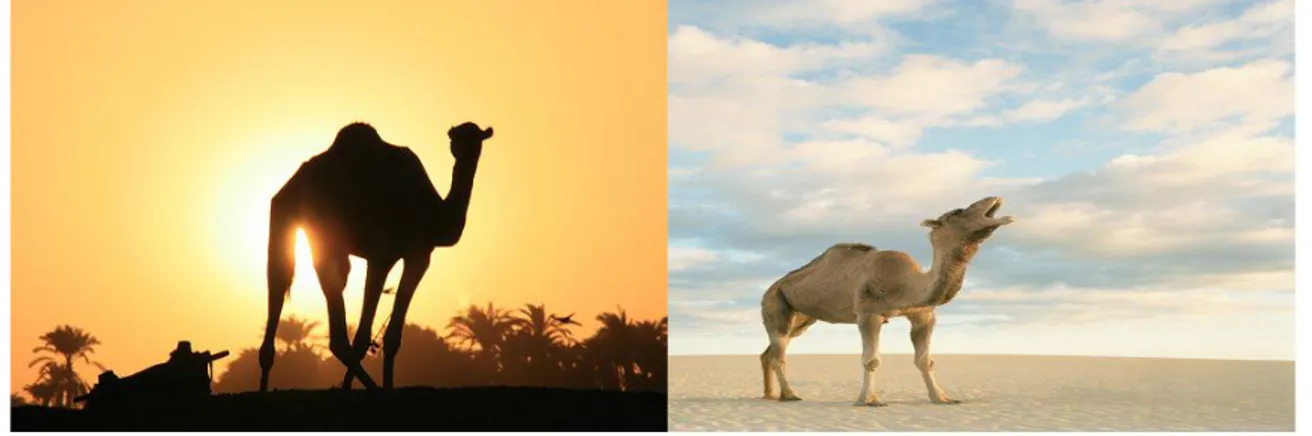
2.2.2 Various body postures :

The body postures of road side animals exhibits very high variability within the same class, and between different classes. Compared to human-face and body, which are almost standard and unique, the animal body have higher appearance variations. It is almost impossible to detect all animal shape categories from one detector based on current image processing technology.

2.2.3 Light conditions (illumination) :

As we know, the image color is very sensitive to the variation of the illumination intensity and lighting directions. The illumination of the outdoor environment is changeable and

(30)

02 | P a g e uncontrollable since it changes along with the vehicle’s lighting, different time of a day, different seasons, and different weather conditions. In addition, the light from the sun or other light source will reflected by the surface of the road or other object, the light will obviously affect the video

and the image quality which may miss our target.

2.2.4 Accuracy of detection :

Accuracy includes minimizing false negative rate and false positive rate. The false positives (a) happen when the system triggers a false giving without any animal. On the other hand, Indicates a false negative (b) when the system does not specify animals that are not in the image.

Figure2.2.Light conditions

(a)

(b)

(31)

02 | P a g e

3. Animal Database Creation

To the best of our knowledge, there is no public animal database which exists in the literature. Hence, a new database for large animal is constructed. The quality of our database directly affect the classifier’s final performance. In order to build a better database, the following critical problems need to be considered:

. Animal species. . Animal origin.

. Image size and proportion. . Animal shapes categories.

we built our database from a large set of images and videos collected mainly from record videos directly from nature or zoos and Internet. and converted to image format using the ratio 1 per 4 continuous frames to avoid repeated sampling. After finishing the video collection, we cut the standard image from the sampled video frames using the constant proportion window (width : height = 10 : 8.5),the window size was determined by the animal body size.

In fact, the hardest problem of animal body detection is the various body postures. It is unrealistic to build an omnipotent classifier which can recognize all kind of animals with random pose.

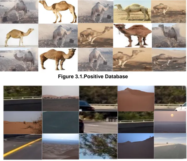
3-1 Positive animal database images :

Each sample positive is a squared image with the size of a typical object in a frame. All sample images will be of the same size. Some noise is present in the form of background pixels in the positive sample images. In order for the classifier to be trained properly, enough of these samples need to be extracted. For the positive samples this is a fixed amount determined by the

(32)

02 | P a g e size of the labeled dataset. There are two factors that determine the amount of these samples in the dataset:

 taking the various of the illumination intensity and lighting directions.  The amount of samples that are taken from the various body postures.

3-2 Negative animal database images :

A good negative (background) database can improve the final detector’s performance to some extent, especially for the detector in the specific detecting environment (driving on the road). Here are some principles of negative dataset creation:

- The most crucial point is that the target object (i.e., animals) can not be contained in the database.

- Any other animals like dog, cat, etc. are excluded from the negative dataset, since they may have similar shapes with big animals.

- Images containing road-objects such as vehicles, pedestrian, traffic sign, road surface, forest, grass, house, tree, etc. constitute the main database.

- Weather, illumination and other environment conditions should be considered as well.

4. Conclusion

In this chapter we had an overview on related works. By going through systems classification, and the objectives that every animal detection system is trying to achieve.

In this same chapter we classified some similar systems. Representing their methods, approaches, advantages and disadvantages.

In the next chapter, we will present our system. The method and the approach we used, trying to highlight the software of this project.

(33)

Chapter 3

System Architecture

(34)

72 | P a g e

1. Introduction

A good architecture leads to a good system. Its advantage appears in the control of the actions or in the automation. Each system can measured from the its architecture and the idea that defines how it work.

In this chapter we will work through the process of designing step by step to achieve the final system. Showing the architecture of the system and system phases (Training, Detection … ect), then passing to equipment and software used to realize this system.

2. System Architecture:

In the architecture of our system, we proposed that work be divided into two phases. The first phase is Training phase, the input in first phase is a dataset and the output is a learned model.

As for the second phase is the use of the result obtained in the first phase in order to access the detection of the object. The input in detection phase is an image and the output is the result of the detection select the object in the image

(35)

72 | P a g e T rai n ing D at a Posi ti v e im ag es Feat u re ext rac ti on Feat u res f us ion dim ensi on reduc ti on C lass if ie r T rai n ing SV M RF Input _imag es Featu res fus ion di m ens ion reduc ti on N eg at iv e im ag e HOG LB P opt iona l T rai n ed Mode l Sli d ing w indow / R eg ions pr o posa ls Feat u re ext rac ti on Reg ions cl as si fi ca ti on N .M.S / Hea t m ap D et ec ti o n res u lt s T rain in g p h ase De te ction p h ase

(36)

72 | P a g e

2.1 Training phase :

2.2.1 Training database :

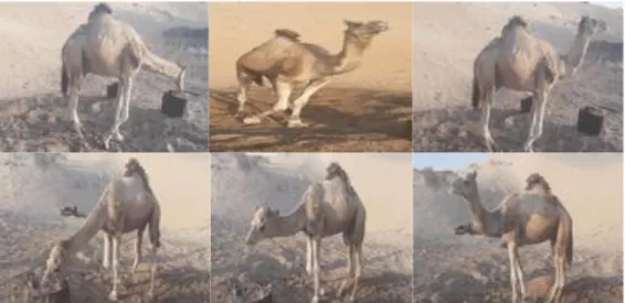
we create a positive database contained 1084 animal images include camel, Figure 3.1

gives some positive images for the various of the illumination intensity and the various body postures. And we create a negative database contained 887 background image , Figure3.2 gives some negative images .All images in database with size 120*100 pixel.

2.2.2 Feature extraction :

The classifier will be trained on features that are extracted from the positive and negative image samples.The quality of these features determines for a large part the performance of the detector. There are many different types of feature extractors that can be used for object

Figure 3.1.Positive Database

(37)

03 | P a g e detection in images. For this thesis two popular feature extractors are compared: the Local Binary Pattern (LBP) and the histogram of oriented gradients (HOG).

All of these three extractors transform an input sample (an image cutout) into a descriptive feature vector that can be used as input for The classier.

2.2.2.1 HOG parameters

The HOG feature descriptor requires several parameters to be tuned in order to obtain the best performance:

Window_size : The size of the window that is used as input. E.g. 64 by 64 pixels. Blocks :

Size: number of cells contained in a block. 16*16 Stride: number of cells overlapped by blocks 8*8

Cells :

Size: number of pixels contained in a cell.8*8 Bins: the number of orientation bins in 0◦ − 180◦ .9

2.2.2.2 LBP parameters :

We initialize our Local Binary Pattern descriptor using a numPoints=24 and radius=8, so that :

 numPoints The number of points in a circularly symmetric neighborhood to

consider (thus removing relying on a square neighborhood).

 Radius The radius of the circle , which allows us to account for different scales.

2.2.3 Classifier training :

Machine learning provide an effective method for processing nondeterministic models which contain incomplete information by describing and predicting a probability density over the variables in questions. Specific to our image target detection, machine learning focuses on prediction (detection), based on known properties learned from the training data. The aim of training process (i.e., learning) is to select suitable features and inform the system which of these features have common characteristic from the positive samples.

(38)

03 | P a g e

2.2 Detection phase :

The detectors are trained on features from images with a fixed size (120x100 pixels). Each of these images contains either an object (filling that image) or not. Since objects can be located anywhere in the image, the entire image needs to be inspected by the detector.

2.2.1 Techniques detection :

Sliding window and selective search These techniques, play an absolutely critical role in object detection and image classification.

Input : Training data

Output : Trained classifier model

Read training data positive images and negative images.

For image in Positive images

Extract features (image).

Add vector features in list vectors images positive. Add value 1 in list labels images positive.

End

For image in Negative images

Extract features (image).

Add vector features in list vectors images negative. Add value 0 in list labels images negative.

End

Concatenate list vectors images positive with list vectors images negative. Concatenate list labels images positive with list labels images negative. Split up data into randomized training and test sets.

Training classifier (X-Train, Y-Train). Test Accuracy (X-Test, Y-Test).

(39)

07 | P a g e

2.2.1.1 Algorithm sliding window:

Sliding windows play an integral role in object classification, as they allow us to localize exactly “where” in an image an object resides.

Utilizing both a sliding window and an image pyramid we are able to detect objects in images at various scales and locations. Most commonly, the image is downsampled(size is reduced) until certain condition typically a minimum size is reached. On each of these images, a fixed size window detector is run (120*100).Now, all these windows are fed to a classifier to detect the object of interest.

2.2.1.2 Algorithm selective search :

Selective Search is a region proposal algorithm used in object detection. It is designed to be fast with a very high recall. It is based on computing hierarchical grouping of similar regions based on color, texture, size and shape compatibility.

Input : Image

Output : List regions of animal detect

Choose a trainer model to detect and classify. Read image input.

Size window (120, 100).

While Size image < Size window

For window in image

Extract features window.

If Classifier (vector features window) predict positive Insert window in list regions detect .

End

Window slid. End

Reduce size image pyramid . End

(40)

00 | P a g e

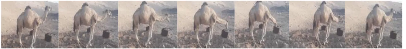
2.2.2 Avoid false positive :

For some images you’ll notice that there are multiple, overlapping bounding boxes detected for each camel in image. In this case, we can apply non-maxima suppression and suppress bounding boxes that overlap with a significant threshold.

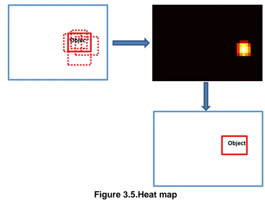
To avoid false positives, a heat map was used. A hit map adds up windows and overlapping windows have a higher value. The values over a certain threshold are kept as true positives.

2.2.2.1 Non maximum suppression :

Because of the sliding window approach, multiple positive detections may be found for a single object. As the window moves step by step over the image, at some point an object might be detected, while at the next step the same object is detected. When the detections are visually analyzed, it is clear that there are margins around each of the objects when there are multiple detections for that object. Non-maximum suppression (NMS) is used to reduce these margins by choosing the detections that are expected to cover the object the best (i.e. the detection located in the center). This method has already provided good results in for example human detection using histograms of oriented gradients and other object detection tasks . Figure 3.3 shows how the suppression algorithm reduces the amount of detections that are found by a detector in an image.

Input : Image

Output : List regions of animal detect

Choose a trainer model to detect and classify. Read image input.

Run selective search segmentation on input image to get list of regions proposal .

For region in Regions Proposal

Extract features region.

If Classifier (vector features region) predict positive Insert region in list regions detect .

End

(41)

03 | P a g e

2.2.2.2 Heat map :

To avoid false positives, a heat map was used. A hit map adds up windows and overlapping windows have a higher value. The values over a certain threshold are kept as true positives.

3. The equipment used for system:

The system we proposed was developed and tested under a rather powerful computer that has the following characteristics:

 Processor: Intel® Core— i7 – 5500U 2.40GHz  Installed memory (RAM): 12 GB

Object Object N M S Objec t Object Figure 3.4.NMS Algorithm

(42)

03 | P a g e

 Graphics Chipset: AMD Radeon R9 4G and software environment:

 Microsoft Windows 10 64-bit Professional with Service Pack 1  Platform Anaconda

 Python 3.6.4  OPENCV 3

3.1 Platform Anaconda :

The open source Anaconda Distribution is the fastest and easiest way to do Python and R data science and machine learning on Linux, Windows, and Mac OS X. It's the industry standard for developing, testing, and training on a single machine.

Anaconda Enterprise is an AI/ML enablement platform that empowers organizations to develop, govern, and automate AI/ML and data science from laptop through training to production. It lets organizations scale from individual data scientists to collaborative teams of thousands, and to go from a single server to thousands of nodes for model training and deployment.

Anaconda distribution comes with more than 1,000 data packages as well as the Conda package and virtual environment manager, called Anaconda Navigator , so it eliminates the need to learn to install each library independently. The open source data packages can be individually installed from the Anaconda repository with the conda install command or using the pip install command that is installed with Anaconda. Pip packages provide many of the features of conda packages and in most cases they can work together.

You can also make your own custom packages using the conda build command, and you can share them with others by uploading them to Anaconda Cloud, PyPI or other repositories. The default installation of Anaconda2 includes Python 2.7 and Anaconda3 includes Python 3.6. However, you can create new environments that include any version of Python packaged with conda .

Anaconda Navigator is a desktop graphical user interface (GUI) included in Anaconda distribution that allows users to launch applications and manage conda packages, environments

(43)

03 | P a g e

Figure 3.6 .Anaconda Navigator

and channels without using command-line commands. Navigator can search for packages on Anaconda Cloud or in a local Anaconda Repository, install them in an environment, run the packages and update them. It is available for Windows ,macOS and Linux.

Navigator is automatically included with Anaconda version 4.0.0 or higher. The following applications are available by default in Navigator :JupyterLab, Jupyter Notebook, QtConsole, Spyder, Glueviz, Orange, Rstudio and Visual Studio Code .

3.2 Python :

Python is an interpreter, object-oriented, high-level programming language with dynamic semantics. Its high-level built in data structures, combined with dynamic typing and dynamic binding, make it very attractive for Rapid Application Development, as well as for use as a scripting or glue language to connect existing components together. Python's simple, easy to learn syntax emphasizes readability and therefore reduces the cost of program maintenance. Python supports modules and packages, which encourages program modularity and code reuse. The Python interpreter and the extensive standard library are available in source or binary form without charge for all major platforms, and can be freely distributed.

(44)

02 | P a g e Often, programmers fall in love with Python because of the increased productivity it provides. Since there is no compilation step, the edit-test-debug cycle is incredibly fast. Debugging Python programs is easy: a bug or bad input will never cause a segmentation fault. Instead, when the interpreter discovers an error, it raises an exception. When the program doesn't catch the exception, the interpreter prints a stack trace. A source level debugger allows inspection of local and global variables, evaluation of arbitrary expressions, setting breakpoints, stepping through the code a line at a time, and so on. The debugger is written in Python itself, testifying to Python's introspective power. On the other hand, often the quickest way to debug a program is to add a few print statements to the source: the fast edit-test-debug cycle makes this simple approach very effective.

3.3 OpenCV :

OpenCV (Open Source Computer Vision Library) is an open source computer vision and machine learning software library. OpenCV was built to provide a common infrastructure for computer vision applications and to accelerate the use of machine perception in the commercial products. Being a BSD-licensed product, OpenCV makes it easy for businesses to utilize and modify the code.

The library has more than 2500 optimized algorithms, which includes a comprehensive set of both classic and state-of-the-art computer vision and machine learning algorithms. These algorithms can be used to detect and recognize faces, identify objects, classify human actions in videos, track camera movements, track moving objects, extract 3D models of objects, produce 3D point clouds from stereo cameras, stitch images together to produce a high resolution image of an entire scene, find similar images from an image database, remove red eyes from images taken using flash, follow eye movements, recognize scenery and establish markers to overlay it with augmented reality, etc. OpenCV has more than 47 thousand people of user community and estimated number of downloads exceeding 14 million. The library is used extensively in companies, research groups and by governmental bodies.

4. Conclusion

In this chapter we saw the architecture of the system and its various components, and system phases (Training, Detection … ect), then passing to equipment and software used, also the general architecture and each step of it.

(45)

02 | P a g e We also discussed how each algorithm works in detail with a pictures clarifying the result that the algorithm give.

In the next chapter we will discuss the implementation and more deep stuff about the system and its functionality.

(46)

Chapter 4

Expriment and result

(47)

04 | P a g e

1. Introduction

:

In this chapter we are going to walk through the implementation of the different classifiers and detectors. Along with the comparison of each result and uses and performances.

2. Implementation

:

After going through the platform and defining it in the previous chapter, now we will explain the implementation of the system. Our system contains two main parts : training and detection .

2.1 Training :

After we did the training we got four trained models which are as follows : SVM+HOG, SVM+LBP, RF+HOG, RF+LBP.

Algorithm For Classification _{Feature extraction} _{Trained Model}

SVM HOG LBP SVM+HOG SVM+LBP RANDOM FOREST HOG LBP RF+HOG RF+LBP Tableau 4.1 Trained model

After that we evaluate the performance of each classifier based on test images and draw Figure 4.1 to show the relationship. This figure indicates that the detection rate increases rapidly when the number of positive sample increases from 100 to 1000.

(48)

04 | P a g e 0 0.1 0.2 0.3 0.4 0.5 0.6 0.7 0.8 0.9 200 400 600 800 1000 1200

Detection rate

2.2 Detection :

After we did implemented algorithm sliding window and algorithm selective search we got eight detector classifier table 4.2 .

Algorithm Trained Model Detector Classifier

Sliding Window SVM+HOG SVM+LBP RF+HOG RF+LBP SW+SVM+HOG SW+SVM+LBP SW+RF+HOG SW+RF+LBP Selective Search SVM+HOG SVM+LBP RF+HOG RF+LBP SS+SVM+HOG SS+SVM+LBP SS+RF+HOG SS+RF+LBP

Table 4.2 Detectors list

Figure 4.1 Relationship between detection rate and the number positive training database

(49)

04 | P a g e

2.2.1 Detectors experiment :

We tried these detectors on three images (Figure 4.2) to various illumination intensity and the various body postures to see the results table 4.3 :

Sliding windows /

regions proposal Region positive N . M . S Heat map

1

2

3

1

2

3

1

2

3

1

2

3

SW+SVM+HOG SW+SVM+LBP SW+RF+HOG SW+RF+LBP SS+SVM+HOG SS+SVM+LBP SS+RF+HOG SS+RF+LBP 151 151 151 151 698 698 698 698 156 156 156 156 1104 1104 1104 1104 132 132 132 132 509 509 509 509 87 75 13 151 408 299 149 698 116 156 35 156 815 960 376 1104 86 27 47 132 322 206 141 509 11 10 3 10 7 4 20 8 11 8 5 8 4 7 18 6 13 13 6 13 2 12 1 1 1 1 1 1 1 1 5 1 1 1 1 1 1 1 4 1 1 1 1 1 1 1 0 0

Tableau 4.3 Test results Figure 4.2 Exprimental images

(50)

04 | P a g e We see in figure 4.3 that the average of regions given by selective search is way more than the ones given by sliding window , This increases the detection time.

All the results of the eight detectors shown in table 4.3. Are represented in the figures were each figure contain how the detectors detect the animal in the experimental images that we talked about previously in Figure 4.2 .

0 100 200 300 400 500 600 700 800 900 Sliding Window Selective Search

Figure 4.3 Relationship between nombre regions and algorithm detection

(51)

00 | P a g e

Figure 4.5 SW+SVM+LBP

Figure 4.6 SW+RF+HOG

(52)

04 | P a g e Figure 4.8 SS+SVM+HOG Figure 4.9 SS+SVM+LBP Figure 4.10 SS+RF+HOG

(53)

04 | P a g e

Figure 4.11 SS+RF+LBP

Figure 4.12 Relationship between detectors and false positive of sliding window

(54)

04 | P a g e

2.2.2 Performance evaluation :

we evaluated the performance of our classifiers following two main criteria: detection speed and detection rate.

Time

Accuracy

1 2 3 1 2 3 SW+SVM+HOG SW+SVM+LBP SW+RF+HOG SW+RF+LBP SS+SVM+HOG SS+SVM+LBP SS+RF+HOG SS+RF+LBP 0.458 2.03 1.33 3.04 3.81 11.85 7.85 15.82 0.54 2.11 1.31 3.14 5.42 20.45 13.07 26.79 0.44 1.76 1.15 2.49 2.90 8.61 5.73 11.36 0.5 0.6 0.85 0.2 0.1 0.45 0.6 0.1 0.15 0.15 0.8 0.2 0.6 0.1 0.45 0.35 0.3 0.1 0.65 0.15 0.3 0.6 0.1 0.1

Figure 4.13 Relationship between detectors and false positive of selective search

(55)

04 | P a g e In the last table we have seen some value that represent the performance evaluation which we will present it in the next charts.

As we see in time of the detection the faster is SVM+HOG and it doesn't really matter with SS or SW. The next chart is about Accuracy.

0 2 4 6 8 10 12 14 16 18 20 Detection time SW+SVM+HOG SW+SVM+LBP SW+RF+HOG SW+RF+LBP SS+SVM+HOG SS+SVM+LBP SS+RF+HOG SS+RF+LBP 0 0.1 0.2 0.3 0.4 0.5 0.6 0.7 0.8 Accuracy SW+SVM+HOG SW+SVM+LBP SW+RF+HOG SW+RF+LBP SS+SVM+HOG SS+SVM+LBP SS+RF+HOG SS+RF+LBP

Figure 4.14 Detection time

(56)

04 | P a g e For the accuracy we notice that the most accurate one RF+HOG but with SW it is way more accurate than using it with SS.

What we can notice in those results that the common point is Sliding window and HOG in both accuracy and time.

3. Conclusion

In this chapter we did go through the implementation with both of it’s part

training and detection. Describing the algorithms we worked with. Passing by the uses to the result ending with discussion, clarifying which algorithm gave the best result.