Dryout droplet distribution and dispersed flow film boiling

AA

Wayne S. Hill

Warren M. Rohsenow

Report No. 85694-105

Contract No. CME-76-82564

Heat Transfer Laboratory Department of Mechanical Massachusetts Institute o A02 Engineering f Technology Cambridge, Massachusetts 02139 August 1982 ENGINEERING PROJECTS NG PROJECTS 4G PROJECTS N4G PROJECTS N4G PROJECTS NG PROJECTS NG PROJECTS NG PROJECTS NG PROJECTS IG PROJECTS PROJECTS PROJECTF ROJEC" )JEr TT .NGINEERI IGINEERI IINEERI NEERI 'EERI ERI RI I

TECHNICAL REPORT No. 85694-105

DRYOUT DROPLET DISTRIBUTION AND DISPERSED FLOW FILM BOILING

by Wayne S. Hill

Warren M. Rohsenow

Sponsored

National Science

Contract No. NSF Grant

D.S.R. Project by Foundation CME-76=82564 A02 No. 85694 August 1982

Department of Mechanical Engineering Massachusetts Institute of TEchnology Cambridge, Massachusetts 02139

ABSTRACT

Dispersed flow film boiling is characterized by liquid-phase droplets

entrained in a continuous vapor-phase flow. In a previous work at MIT, a

mo-del of dispersed flow heat transfer was developed, called the Local Conditions

Solution, which is amenable to hand calculation of wall temperatures. This

solution identifies a single nonequilibrium parameter which depends solely on conditions at dryout, particularly a characteristic droplet diameter. Pre-vious to the current study, no simple model including mechanisms occurring

upstream of dryout had succeeded in predicting the droplet distribution at dryout.

The Local Conditions Solution is rederived to identify which droplet diameter characterizes the distribution of droplets at dryout for purposes

of dispersed flow heat transfer analysis. Based on mechanisms of droplet

entrainment and deposition, the dryout droplet distribution is derived.

This distribution is integrated to obtain the characteristic droplet

dia-meter. A simple method of calculating the characteristic droplet diameter

is presented.

With the droplet distribution model, the Local Conditions Solution

is compared with three correlations and seven data sets. In general, the

Local Conditions Solution predicts wall temperature data to within about

5% better than the three correlations.

It is found that some data display a type of behavior not predicted by the Local Conditions Solution. This may be caused by the enhancement of

ACKNOWLEDGEMENTS

The authors are grateful to Professors Peter Griffith, Borivoje

Mikic, and Ain Sonin for their help and advice. Thanks are also due to

Dr. Lawrence Hull for his comments and suggestions. The typing was done

This research was supported by a grant from the National

Science Foundation.

TABLE OF CONTENTS Abstract 2 Acknowledgements 3 List of Figures 7 Nomencl ature 8 CHAPTER I: INTRODUCTION 12

1.1 Dispersed Flow Heat Transfer 12

1.2 Review of Related Work 18

1.3 Objectives of Research 21

CHAPTER II: BASIC PRINCIPLES OF TWO PHASE FLOWS 23 CHAPTER III: REDERIVATION OF THE LOCAL CONDITIONS SOLUTION 30

3.1 Liquid Mass Balance 30

3.2 Evaporation of Droplets 31

3.3 Flow Heat Balance 32

3.4 Droplet Slip

3.5 Drag Coefficient 35

3.6 Droplet Nusselt Number 36

3.7 Nusselt Number Droplet Diameter 37

3.8 Droplet Reynolds Number 39

3.9 Characteristic Droplet Diameter 40

CHAPTER IV: DERIVATION OF DRYOUT DROPLET DISTRIBUTION 42

4.1 Entrained Droplet Diameter 43

4.2 Deposition 48

4.3 Droplet Entrainment Rate 53

4.4 Dryout Droplet Distribution 55

4.5 Characteristic Droplet Diameter 57

4.6 Examination of Assumptions 60

CHAPTER V: APPLICATION TO DISPERSED FLOW FILM BOILING ANALYSIS 65

5.1 Nonequilibrium Parameter 65

5.2 Actual Quality 66

5.3 Vapor Temperature 66

5.4 Wall Temperature 69

5.5 Varying Heat Flux 70

CHAPTER VI: COMPARISON WITH OTHER MODELS AND PUBLISHED DATA

6.1 Dougall-Rohsenow

6.2 Groeneveld and Delorme 6.3 Chen et al

6.4 Comparison with Data

6.5 Summary of Comparisons CHAPTER VII: APPENDICES SUMMARY APPENDIX I: APPENDIX II: APPENDIX III:

ANNULAR FLOW MODEL

DRYOUT FILM SLIP RATIO AND RELATIVE VELOCITY SAMPLE CALCULATION

REFERENCES

99

102

LIST OF FIGURES

Figure Page

1-1 Inverted Annular Flow 14

1-2 Annular Flow 15

1-3 Limits of Complete Equilibrium and Complete Nonequilibrium 17

3-1 Comparison of Nusselt Number Correlations 38

4-1 Results of Annular Flow Model for Relative Velocity

Between Vapor and Film 46

4-2 Four Regimes of Deposition Velocity 49

4-3 Droplet Deposition Mass Balance 51

4-4 Distribution Factor for xb = 0.20 61

4-5 Distribution Factor Multiplier for Dryout Quality 62

4-6 Mass Distribution vs. Droplet Diameter for

Xxb = 3, Web = 105, and xb = 0.5 63

5-1 Tangent Approximation to Actual Quality vs.

Equilibrium Quality, for K = 0.5 67

5-2 Actual Quality vs. Equilibrium Quality 68

6-1 Comparison with Bennettetal, Case I 79

6-2 Comparison with Bennett et al, Case II 80

6-3 Comparison with Bennett et al, Case III 82

6-4 Comparison with Bennett et al, Case IV 83

6-5 Comparison with Groeneveld [5] 85

6-6 Comparison with Era et al [3] 86

6-7 Comparison with Hynek [1] 87

A3-1 Actual Quality vs. Equilibrium Quality for

NOMENCLATURE

A Cross-sectional area (ft 2)

Ac Dimensionless acceleration group (Eq.(2-9))

B Mass transport number

Cd Droplet mass concentration in the core flow (lbm/ft3₎

CD Droplet drag cofficient

C, iDroplet correlation coefficient

C Specific heat at constant pressure (Btu/lbm*R)

p2

d Droplet mass deposition rate (lbm/hr ft2)

D Droplet diameter (ft)

D Characteristic droplet diameter (ft)

Dy TTube diameter (ft)

e Mass entrainment rate (lbm/hr ft2)

E Mass entrained per unit change in quality per unit time (lbm/hr)

f Distribution factor for xb = 0.2 (Eq. (4-45)) f Friction factor (Eqs. (Al-5), (Al-6))

F Distribution factor

g Gravitational acceleration (ft/hr

)

G Mass flux (lbm/hr ft2)

Gr Dimensionless gravity group

h Heat transfer coefficient (Btu/hr ft 2* R)

ig Heat of vaporization (Btu/lbm)

k Thermal conductivity (Btu/hr ft0R)

kd Deposition velocity (ft/hr)

K Nonequilibrium parameter (Eqs. (3-23), (5-1))

L Length (ft)

m Droplet mass (lbm)

n _{Droplet site distribution (hr~} ft~)

Nu Nusselt number

p Pressure (lbf/in

)

q d Heat transfer to a droplet (Btu)

d Average heat transfer rate to a droplet (Btu/hr)

q " Wall heat flux (Btu/hr ft2₎

rb Radius of curvature at dryout (Eq. (5-4))

Re Reynolds number

Re Reynolds number defined by Eq. (3-18)

Reb Dryout Reynolds number (Eq. (4-12))

s Slip ratio t Time (hr)

T Temperature (*F or *R)

u* Friction velocity (Eq. (4-15))

V Velocity (ft/hr)

We Weber number

Web Dryout Weber number (Eq. (4-11))

x Quality

z Axial position (ft)

Greek

a Void fraction

n Entrainment fraction

A Deposition parameter (Eq. (4-23))

y1 Viscosity (lbm/hr ft)

p Mass density (lbm/ft3)

a Surface tension (lbm/hr2)

T Shear stress (lbf/ft2

)

T+ Dimensionless relaxation time (Eq. (4-16))

Distribution factor multiplier for dryout quality (Eq. (4-46)) Nonequilibrium variable of Groeneveld and Delorme [10],

(Eq. (6-5))

Subscripts

b Burnout or dryout

c Core

Dropl et Equilibrium Film Saturated vapor Homogeneous Film-vapor interface Liquid Nusselt Number Relative Saturation Steady State Total Tube Vapor Wall Arithmetic Mean Area Mean Volume Mean

CHAPTER I INTRODUCTION

1.1 DISPERSED FLOW HEAT TRANSFER

Dispersed flow film boiling is a regime of two phase heat

trans-fer occurring in such applications as once-through steam generators,

cryogenic machinery, and in the hypothetical loss-of-coolant accident (LOCA) in nuclear reactors. It is characterized by a dispersion of liquid-phase droplets entrained in a continuous vapor-phase flow.

Because the liquid phase is not in physical contact with the

heated wall surface, dispersed flow film boiling can result in high wall

temperatures. Even in low pressure steam-water flows, wall temperatures

can become high enough for the heated wall material to melt.

Conse-quently, a great deal of effort has been expended in recent years to model dispersed flow heat transfer, particularly for nuclear reactor safety analysis.

Dispersed flow heat transfer can occur in a wide variety of physical geometries, most notably in the complicated geometries of

reactor core rod bundles. The most commonly studied geometry for

funda-mental research, the simplest geometry, is vertical upflow in circular tubes with constant wall heat flux. This is the geometry considered in this study.

pre-cede the formation of dispersed flow [1]. The wall heat flux and/or the initial wall temperature determines which of these flow regimes occurs.

If the initial wall temperature is high, or the imposed heat flux is very high, inverted annular flow may precede dispersed flow.

This pattern is shown in Figure 1-1. In inverted annular flow, the

point at which the liquid leaves contact with the wall, the dryout

or burnout point, is very near the beginning of the heated section. Wall temperatures are high enough to cause the liquid to form a core in the center of the tube, with a vapor annulus next to the wall.

Be-cause of the high density ratio between the liquid and vapor, vapor

velocities are much greater than the liquid velocities, and eventually

the liquid core becomes unstable. Once the core flow ruptures,

drop-lets are rapidly formed, and dispersed flow is established.

If the inital wall temperature is not very high, or if wall heat fluxes are not very high, annular flow precedes dispersed flow. This pattern is shown in Figure 1-2. As liquid entering the bottom of the tube is heated, vapor bubbles begin to form at the walls. In the nucleate boiling region, liquid remains in contact with the walls,

re-sulting in good heat transfer and low wall temperatures. Because of

the low wall temperatures, the liquid and vapor are essentially at saturated conditions. As more vapor is generated, the vapor collects in the center of the tube, surrounded by a liquid film in contact

0 0 00 0 0

vapor

Dryout

l

liq

uid

liquid

fIt

Figure 1-2. Annular Flow

with the wall. The vapor velocities are again much larger than the liquid velocities. Instabilities occurring at the liquid-vapor inter-face cause droplets to be torn from the film and entrained in the vapor

core. Eventually, evaporation and entrainment deplete the liquid film,

and dryout or burnout occurs. In this study, it is presumed that

an-nular flow precedes the establishment of dispersed flow.

The most serious complicating factor in the analysis of dis-persed flow film boiling is the presence of the liquid droplets in the

otherwise continuous vapor flow. Because the liquid is essentially at

saturation, while the vapor can be considerably superheated, the drop-lets behave as a distributed heat sink in the vapor flow. While the

droplet volume flow rate is virtually negligible compared to the vapor

volume flow rate (void fractions are on the order of .90 to 1.0), the liquid mass flow rate can be comparable to the vapor mass flow rate (dryout qualities can be as low as about .05). Thus, the magnitude of

the distributed sink can be considerable. Since most of the heat

trans-ferred to the droplets must first be transtrans-ferred to the vapor, the flow is generally not in complete thermal equilibrium. Thus, the flow is

generally somewhere between thermal equilibrium and nonequilibrium,

as illustrated qualitatively in Figure 1-3. The degree of thermal

non-equilibrium depends on the individual mechanisms that occur in

dis-persed flow. The analysis becomes even more complicated when the

ef-fects of radiation from the wall to the droplets and direct drop-wall

Complete

Dryout

1.2 REVIEW OF RELATED WORK

EXPERIMENTAL

Experimental data for dispersed flow heat transfer are

avail-able for many fluids over a large range of flow conditions and

dif-fering physical and flow geometries.

Quite a lot of data have been

1000 psia. Forslund [4] and Hynek [1] have presented data using

nitrogen at low pressures.

Groeneveld [5] and

Cumo et al [6] have

published data using Freon 12, while Koizumi et al [7] used Freon

113.

There are basically two types of approaches which have been

utilized in analyzing dispersed flow heat transfer data. These can

be divided conveniently into correlative and phenomenological analyses.

CORRELATIVE

Correlations .usually begin with an assumption of the general

form of the behavior of the flow. Many correlations begin with an

ac-cepted equation for pure vapor heat transfer, such as the McAdams or

Dittus-Boelter correlation, which is then modified to account for

such behaviors as thermal nonequilibrium, droplet slip, and entrance

length effects.

Free parameters are then evaluated using data from a

While these solutions are usually simple to apply and are, therefore, attractive, they are generally not valid outside of the data base from

which they were developed.

A large number of correlations have been presented in the litera-ture, a partial list of which is presented by Groeneveld and Gardiner [8].

Two correlations which will be considered in this study (see Chapter VI) are those of Chen et al [9] and Groeneveld and Dolorme [10].

Both of these correlations explicitly account for nonequilibrium in the flow, and were developed by back-calculating vapor temperatures from wall temperature data, knowing wall heat flux and assuming a

single-phase wall heat transfer coefficient.

PHENOMENOLOGICAL

Most phenomenological models begin with an assumed model of the

heat transfer processes occurringin the flow. Using correlations to

characterize individual mechanisms, the models follow the flow as it

moves down the tube. This usually requires a step by step solution scheme that must be implemented on a computer. The advantage of this

approach is that, because specific heat transfer mechanisms are

modeled, these models sometimes do better over a wider range of

con-ditions than do correlations.

One of the first of these models, by Dougall [11], (the

assump-tion of thermal equilibrium. Originally, this equaassump-tion was shown to be

an asymptote at high quality for film boiling data at low quality. It

was not intended for prediction at low quality. Since this correlation,

though not recommended, is still used widely, results of this study

are compared with those of Dougall 's equation in Chapter VI.

A discussion of the development of phenomenological models of

dispersed flow film boiling is presented by Yoder [12]. Yoder created

a computer model of dispersed flow heat transfer which included five

types of heat transfer interactions. These were: convection from the

tube wall to the vapor; convection from the vapor to the droplets; radiation from the wall to the droplets; direct drop-wall interaction;

and axial conduction along the tube wall. In general, excellent

re-sults were obtained using this model. Yoder found that ignoring

radia-tion, drop-wall interacradia-tion, and axial conduction did not result in a serious loss of accuracy of the model's predictions.

This led him to develop a new phenomenological model, based on

a,two-step heat transfer process. Heat was assumed to be transferred from the wall to the vapor only, and from the vapor to the droplets. This model results in a single differential equation for actual quality

vs. equilibrium quality, a measure of thermal nonequilibrium. While

this differential equation cannot be analytically integrated, it

de-pends on only one parameter, denoted the nonequlibrium parameter K,

which is constant for a given flow situation. Given the conditions at

quality, the vapor temperature calculated, and the wall temperature

pre-dicted at any position downstream of the dryout location. This model

was called the Local Conditions Solution.

The

main difficulty of the Local Conditions Solution, and most

other phenomenological models of dispersed flow heat transfer, is its dependence on the knowledge of a characteristic droplet diameter at the dryout point. Most researchers simply back-calculate the droplet

diameter from other considerations. Yoder's model of the dryout

drop-let diameter was tedious to apply and initially required numerical ex-perimentation to find an optimal value of a critical Weber number for

droplet entrainment.

The purpose of the present study is

to develop a phenomenological

model of annular flow to predict the characteristic droplet diameter at dryout.

1.3 OBJECTIVES OF RESEARCH

In order to include properly the pertinent physical mechanisms in annular flow which give rise to the droplet distribution at dryout,

the phenomenological approach was used in this research. The objectives

were as follows:

* To rederive the Local ConditionsSolution to determine which

dryout for purposes of dispersed flow heat transfer.

" To develop an analytical model based on mass, momentum,

and energy conservation equations and recent correlations which describe specific mass transfer mechanisms to

pre-dict the droplet distribution at the dryout point.

" To apply this model and appropriate simplifications to

the Local Conditions Solution, to result in a simple, accurate model for predicting dispersed flow heat

trans-fer behavior.

" To apply the LocalConditions Solution to published data and

CHAPTER II

BASIC PRINCIPLES OF TWO PHASE FLOWS

In order to clarify later discussion of the mechanisms occur-ring in annular and dispersed flows some basic principles and nomen-clature of two phase flows are described here.

The total mass flow rate is usually represented by the flow rate

per unit cross sectional area, the mass flux.

G - - (2-1)

AT

The vapor and liquid mass flow rates are sometimes expressed in terms of separate mass fluxes,

w G -t and (2-2) AT w G z - .(2-3) AT

The vapor and liquid flow rates are related to the total flow rate by

the quality (or actual quality).

w

x w- (2-4)

(1 - x) - (2-5) wt

Thus, the vapor and liquid mass fluxes are

G = xG , and (2-6)

G = (1- x) G (2-7)

The equilibrium quality xe is the quality that would occur if the

liquid and vapor are in thermodynamic equilibrium. A simple heat

balance shows that

I'

4 q

x (z - z ) , (2-8)

GDT _Ifg

where q is the wall heat flux (constant), z is the axial position

along the tube, and z is the location where the enthalpy is the saturated liquid enthalpy, or x = 0.

Defining the acceleration group Ac as

11

Ac q , (2-9)

Gi fg

4

Ac

Xe

=-

(z

-

Because the liquid and vapor are essentially at saturation in

annular

flow, the actual quality and equilibrium quality are equal in

annular

flow. However, significant superheating of the vapor can occur in

dispersed flow, so the actual and equilibrium qualities are not equal

in

dispersed flow. It

is

the prediction of this departure from

equi-librium which is the ultimate purpose of this study.

In

annular flow, it

is

often necessary to distinguish between

the liquid in

the film and the liquid entrained as droplets in

the

vapor core. This is

done using the entrainment fraction

wentrained

(2-11)

The fraction of the tube cross section that is

covered by vapor is

termed the void fraction

A

1

A =- 1 + ,V ( 2-12)

AT 1 + s

where the slip ratio s is the ratio of average vapor and liquid

velocities.

V

In dispersed flow, the slip ratio is an average droplet slip ratio,

V

s = (2-14)

d - V

Because sd = 1, the void fraction in dispersed flow is approximately

the homogeneous void fraction,

+l1-x Pv (2-15)

x p

Because the liquid in annular flow is distributed between the liquid film and droplets entrained in the core flow, speaking of a single slip ratio in annular flow does not seem to be physically meaningful.

Conse-quently, the core and film void fraction are sometimes differentiated in

annular flow. The core void fraction is

A 1

-= =. (2-16)

c _{c 1 + n s}

Neglecting the droplet area in the core (ac= 1), the film void fraction is approximately

A 1

a f _c 0 , (2-17)

AT

_x

_pt

_f

s V

sf-

1 9 (2-18)

It is often necessary to express the vapor velocity or the rela-tive velocities between the vapor and a droplet or the liquid film. The vapor velocity is

Gx

V

v v

(2-19)

where a c f _{in annular flow, and a ~ h}

The relative velocity between the vapor and

V(r v :1 G x

rf _vec

bete

and similarly the relative velocity between

in dispersed flow.

the liquid film is then

1)

(2-20)

the vapor and a droplet is

Vrd

v(l

(-

-2-)

sd va sd

(2-21)

Because sd is near unity, (1 - -) (sd - 1). This approximation will

d

prove to be useful later on.

While quality, void fraction, and slip ratio (and entrainment

fraction in annular flow) are interrelated, considerations of mass and

energy conservation are not sufficient to determine completely the inter-relationship. To close the set of equations requires consideration of momentum conservation. In dispersed flow, this comes in the form of

a droplet drag coefficient. In annular flow, the situation is further

complicated by separate liquid film and droplet flows. A model has been written for this study based on that of Wallis [13]. In this model, the pressure gradients of the core flow and total flow are modeled separately and equated to yield another relation. With the addition of an assumed entrainment fraction profile, the set of equations is closed. Two

ver-sions of the model have been written, one without accelerational effects, and one including accelerational terms, and are described in Appendix I. Unfortunately, neither modelyields an explicit analytical result, but

requires computer solution.

While the numerical results of both models are of questionable

accuracy in describing the phenomena modeled, they do indicate the proper

trends, and gi.ve some indication of the importance of accelerational

ef-fects. In general, the results of both models are quite similar. Film

void fractions predicted by both models agree to within one percent,

and relative velocities between core and film generally agree to within

about six percent. Thus, by and large, accelerational effects can be

ignored.

One interesting result is obtained analytically from the

non-accelerational model. Near dryout, where both a and n approach

unity, L'Hopital's rule can be used to obtain the result

s -

W

Sx - 1

This result, derived in Appendix II, will prove useful in describing the

CHAPTER III

REDERIVATION OF THE LOCAL CONDITIONS SOLUTION

The droplets in the core flow are not all of one

size:

an entire distribution of droplets is entrained. Until it is known which droplet diameter properly chatacterizes the distribution for

pur-poses of dispersed flow film boiling analysis, the problem description is incomplete.

In order to answer this question, the Local Conditions Solution is derived here including the behavior of a distribution of droplets.

Wherever the diameter per se of a droplet is intended, D₁ (the

arith-metic mean diameter) is inserted: similarly, whenever the surface area

or volume of a droplet is intended, D₂ or D₃ (the surface mean or

volume mean diameter) is inserted, respectively. Thus, when the

deriva-tion is complete, the characteristic droplet diameter, D*, will be

ap-parent.

3.1 Liquid Mass Balance

The liquid mass flow rate crossing a plane is

w = - n p D = - DT G(1 - x) .(3-1) A m6 ta n 4 T

drop-lets crossing a plane per unit time, n , is constant. From this, it is clear that (3-2) 1 x 1/3 D3 -- D 3 b (1 _{~ b)} Differentiating Equation (3-1), dw Tr

2Gdx

1-x

From Equation (3-2), then

dwz dz .6 F' P D3b 1 : x) I x (1 -Xb 1/3 dx (3-3) 3.2 Evaporation of Droplets

The time required for a droplet to travel a distance Az is

At = Az/Vd. The heat transferred to a droplet in a distance Az is

thus

qd = TrD hd(Tv - Ts A) Vd

so that the mass evaporated from a droplet in traveling a distance Az isAqd -TD2_hd(Tv - Ts )Az ifg _*1 fg Vd

Assuming that droplet velocity is independent of diameter, and

inter-grating over all droplets,

dw . I D2 hd(T - T

- -d (3-4)

dz _{i fg Vd}

Equating this to Equation (3-3),

dx D₂2 hd(Tv _- TS) -= 6 ₂ d dz D 3 Y2fg Vd

1

x

1/3

3.3 Flow Heat Balance

Because some heat goes into superheating the vapor, the actual vapor flow rate is less than that which would occur in an equilibrium situation. Thus, wq 2 < Wv =- D T Gxe and equil1 4 vactual = A DT Gx

w 'actual1 iT ₂₀ =-D ( 4 z equil 4 DT 2_{G (1 - xe)}

A simple heat balance yields

(i _{- i )(w} or uw ) _i i -i 1_fg Assuming that x _e equil -1 i - ig = C p (T

Substituting this into Equation (3-5),

dx D2 hd 1 - x

-- = 6 ₂

dz D3 2 P2pv d D3b

Identifying, from Equation (2-10),

and defining and 1/3

~

is the characteristic droplet diameter for the droplet

actual) ' (3-6) T )19 TV - T =cs Cpv (Xe x 1).(3-7) (e

-

/

Nusselt number, 2 1 D₃bD₃2 _DNu - x = - -- _{2 2} 3 D T _{D 2} Pz Re D x 1 3 Ac Pr - /3 b) 3v Nu(1 - x (3-9) dx dxe 3.4 Droplet Slip

Based on a force balance on a droplet, Yoder [12] found

D3 Vd dVd _ dz 6 D3g(pk - v) 7T ₂ + -D 8 CD v 2d d

where CD is the droplet drag coefficient. Assuming that

dx dx _ e dz dz

d

1

the following result is obtained. 4 3 G2 CD

_(3-10)

Of the previous assumptions, Yoder supports the second rather con-vincingly. The first assumption is only valid in annular flow. In

- 1)2 and dx e dx 16 D --1 + V , -(l

dispersed flow, the accuracy depends rather strongly on the degree of

departure from thermal equilibrium and will, in some cases, cause

signif-icant errors. However, without this assumption, no result could be

ob-tained in closed form. Thus, this model is used in the present work with

some reservations.

The effect of gravity is negligible if k «1.

CD G2 x2

This is usually the case except at low qualities. Equation (3-10) then simplifies to

s= + Ac -- - . (3-11)

3 p v _{x CD DT}

The term under the radial is usually small compared to one, so the

droplet slip ratio is usually near unity.

3.5 Drag Coefficient

Yoder used the drag coefficient of Ingebo [14] for accelerating spheres,

27

CD= _{Red .84}

CDmi _n = 0.40 .

However, because the accelerations encountered in annular flow are

sig-nificantly smaller than those in Ingebo's experiments, the hard sphere correlation used by Hynek [ 1 ] was used in this study.

C

~ 24 ( 1

+

.142 Re .698

3.6 Droplet Nusselt Number

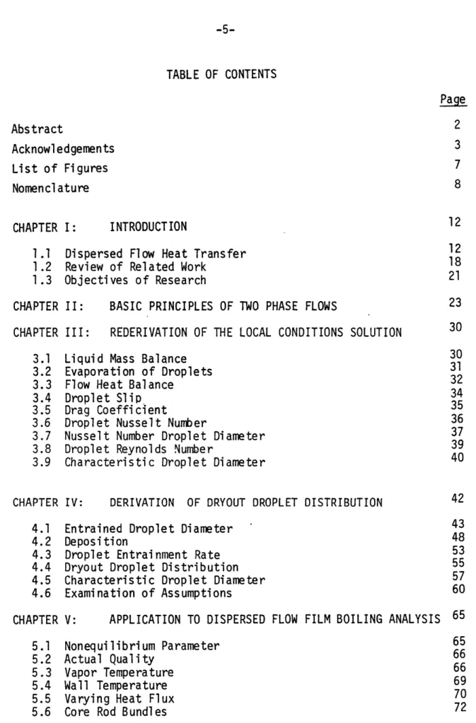
As in Yoder, the droplet Nusselt Number will be characterized by the Ranz and Marshall hard sphere correlation [15],

Nud = 2 + .6

1/2 Prvf1/3

modified by Yuen and Chen [16] to account for mass transfer by

1 + B = 1 + C P(T -Ts

)

Since the droplet slip ratio is near unity,

1 16 p 1 D - 1 -- Ac- -sd 3 pV x CD DT so G x 16p , 1 D V -~ Ac -- . (3-14) r vah 3 pv x CD DT

It would be convenient if Nud could be approximated using a constant

drag coefficient, say CD = .40. As shown in Figure 3-1 , the Nusselt

number is well chararacterized by

.63 G x D 6 p 1 1/3 Nud = - Ac - - Pr 1 p - Ts( V 3 pk .4 x Dvf fg From Equation (3- 7), C pv(T -T) e 1 + ~ = - e fg X so 16 9 1 D 1/2 1/3

Nud = .63 -Ac -- ) Pryf (3-15)

x e ( 11ah 3 p v .4 x D T

3.7 Nusselt Number Droplet Diameter

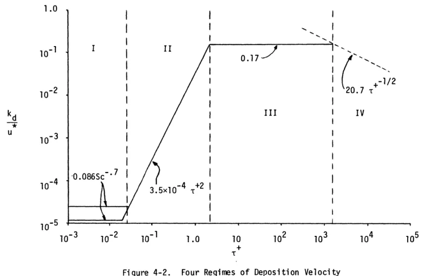
The Nusselt numberdroplet diameter is defined so that the heat

transfer to a droplet of diameter DNu is the average heat transfer per

U 4-Q) 0 r 10 Nud = 2 + 0.6(RedHS Pr S.. co 5 0 aNu = 0.63(Red )//2 Pr1/3 c3 d dCd 4) 10 100 1000

Red Based on Cd o'40

Nud(DNu )k V(T - Ts D~uS 2 Nu(D)k 7rD D v(T -T)n(D)dD

f

n(D)dD

where n(D) is the droplet size distribution. Since, from Equation (3-15),

Nud Il the above relation suggests that

DNu7/4 n(D)D 7/4dD n (D) dD

(3-16) DNu 7/4 D2

Since void fraction is close to unity, the variation of void fraction

with quality may be neglected. Then, from Equation (3-15),

Nud ~ 23/4 (3-17)

3.8 Droplet Reynolds Number

From the definition of the droplet slip ratio,

V Gx

sd Pvahsd

Neglecting droplet slip,

, GxD

ReD Th (3-18)

2

Again neglecting the variation of void fraction with quality,

Re ~ x

Equations (3-17) and (3-19) yield

ReD _~ e 1/4 3/4 Nud X X b D3/ 4 R 2b db D234Nu _db (3-20)

3.9 Characteristic Droplet Diameter

Sustituting Equations (3-20) into Equation (3-9) results in

21 D3bD0 DN 3 _D D22 D2b3/4 D23/4 1 -xb)

1/3

Assuming that all droplet diameters vary, like D3, as (1 - x )1/3

Equation (3-21) may be written with x = xb = Xe at dryout, as follows:

x3/4x d X3/ Xe dx K 7/2 X - x

(1 -

Nud at dryout from Equation (3-15), the nonequilib-(3-19)

* 5/4 P9 3/4 2/3

D w (Ac -) Pr

K= .554 pv 5/12v 1 /2 Reb ,3-23)

DT b xb

where the dryout Reynolds number is

G _{xb DT}

Reb = , (3-24)

and where the characteristic droplet diameter is identified to be

D D 12/5

S( 3-25)

02

Once the characteristic droplet diameter is known, the non-equilibrium parameter can be calculated, and Equation (3-22) can be

CHAPTER IV

DERIVATION OF DRYOUT DROPLET DISTRIBUTION

Four distinct mechanisms can be identified which could conceivably have an impact on the droplet distribution at dryout. These are:

- Droplet entrainment from the liquid film, - Coalescence of droplets in the free stream, - Break-up of droplets in the free stream, and - Deposition of droplets back onto the liquid film.

Droplet evaporation does not play a part, because the vapor and drop-lets are essentially saturated upstream of dryout. Because of the high core void fractions common in annular flow (generally > .90) droplet coalescence probably does not occur to a degree great enough to affect substantially the droplet distribution.

The break-up of droplets in the free stream is apparently controlled by a critical Weber number criterion [17],

2

p VrdD G2_x2_{D(l -} 1

_/sd(

We crit < v CTrg c d.(-) Pyaa

Since the entrainment of droplets from the liquid film is largely con-trolled by a Weber number criterion as well (as will be shown in the next section), and the film slip ratio is large compared to the droplet slip ratio, droplets entrained at one point travel a long distance be-fore break-up. From Eq. (4-1),

xbreak-up _{__s}

.

(4-2)

Xentrain ₁

-s d

Consequently, if any droplet break-up occurs at all, it is the large droplets that were initially entrained (many of which have already been redeposited) that break up first. Thus, for now, break-up will be ignored, an assumption to be reexamined later.

Thus, the mechanisms that are considered here are the entrainment of droplets from the liquid film to the vapor core and the deposition of droplets back onto the liquid film.

4.1 ENTRAINED DROPLET DIAMETER

While several mechanisms of droplet entrainment have been identified (e.g., wave undercutting, droplet impingement, and liquid bridge dis-integration), it is generally believed that the shearing off of roll wave tops is the predominant mechanism occurring in annular flow.

Kataoka, et al. [18] expressed the distribution of droplets entrained at a point (translated into the current nomenclature) as a modified Weber number criterion. D. p G x DT 2/3 _{p 1/3 y /} D, _S Ci Gz _{i Gx} ( ₁₁ ) ( ) ( - ) , (4.3) v _{v l} where C1 = .0031 for Di , (4-4) C₂ = .0040 for D2 , and (4-5) C₃ = .0053 for D3 - (4-6)

This correlation was developed from adiabatic air-water data, where the large density ratio results in void fractions near unity and very large film slip ratios, and consequently

Gx (l__) Gx (4_7)

V rf ~~ v a sg fpv

Because the area of application of this study is largely in high pressure applications, where smaller density ratios result in smaller void

frac-tions and film slip ratios, this relative velocity effect requires further investigation.

Yoder used Ahmad's slip ratio [19] to characterize film slip.

(

P.205 -G DT -.016

sf = ) (-)

However, this slip ratio was derived from void fraction data at low qualities. Because void fraction is quite insensitive to slip ratio, but slip ratio is sensitive to void fraction, the application of this correlation to relative velocity estimation is of questionable validity.

Instead, for this study, an analytical result from the void frac-tion model, derived in Appendix II, will be used. The dryout film slip ratio is

sfb b

G x G xb Vrfb = p b b v v fb v p X b - xb + 1 v (4-8)

In Figure 4-1, Vrf /Vrfb is plotted against x/xb for two cases of practical interest. These data are results of the annular flow model with no acceleration. As is apparent from the figure, Vrf/V rfb is not a strong function of the gravity group,

Gr

- PP g D T

Picking an average case, a curve fit yields

V _rf g_b

V

1+1.23(x/xb)

(4-9)

For high pressure applications, Eq. (4-3) is modified by replacing

V2 (Gx/p )2 with V2 found from Eqs. (4-8) and (4-9). This leaves

rf v rf op _{GxDT 2/3} b "v pt- 1/3 Pv b + -)2 -2+2.46( )2) Pt xb Xb yv 2/

Bennett et al [2] Case III: Gr=0.063 Bennett et al [2] Case IV: Gr=0.0018 0.9 0.8 0.7 0.6 0.5 0.4 0.3 0.2 0.1 0 0.5 0.6 0.7 0.8

Figure 4-1. Results of Annular Flow Model for Relative Velocity Between Vapor and Film

Vrf Vrfb 2 Vrf _ x

1+1.23/\2

or D. C. p 1/3 yi 2/3 (p - b + 1)2 (Re 2_/

_{(_)}

₍

lb

(/3

where the dryout Weber number is

We G2_{xDT (4-11)}

Wb Pv a

and the dryout Reynolds number is

Reb GxbDT (4-12)

biv

One reassuring feature of this droplet correlation is that, because, from Eqs. (4-10), (4-11) and (4-12),

D 1

IT'

T DT

it is unlikely that a droplet diameter will be predicted to be larger than the tube diameter, thus averting a preposterous limiting behavior.

Consideration of the rate at which entrainment occurs will be de-layed until after droplet deposition is considered.

4.2 DEPOSITION

Droplet deposition is usually characterized by a deposition velocity kd

d = kdCd (4-13)

where d is the mass deposited per unit film area per unit time, and Cd is the droplet mass concentration in the-core flow,

C = Entrained Mass Flow Rate

d Core Area-Droplet Velocity

6p D3 2 2 P9 D3

= = - _(4-14)

T

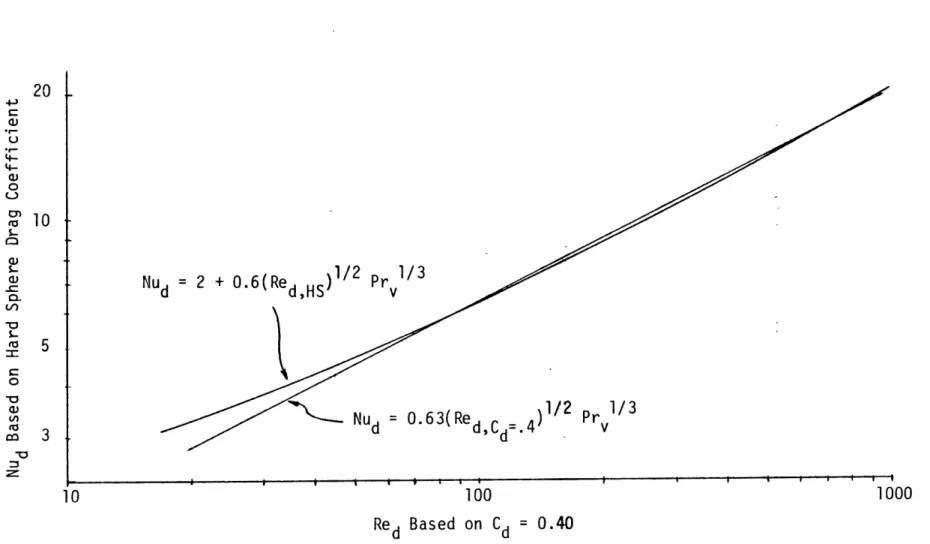
D

where n is the number of droplets crossing a plane per unit time. McCoy and Hanratty [20] identified four regimes of deposition velocity, Figure 4-2. In the graph, u* is the friction velocity,

(Gx)71 4

y

u*2= .03955 p2 D1 v , (4-15)

v T

and T+ is the dimensionless relaxation time

+ D 2 PvP1u*2 -3 PRID2(Gx) 7/

8

= 1pu = 2.20x10 4 4 . (4-16)

v pv D T I'v

The first regime is controlled by Brownian motion, and thus occurs only in submicron particles. The second regime also occurs only in small

|0+-1/2

10-2

20.7

I-3

10- 3

10-

10~

1.0

10

102

10

₁₀₄

₁₀₅

particles or in low speed flows. In fact, results of the annular flow model described in Appendix I indicate that only the third and fourth

regimes occur in annular flow, and the third regime appears to be strong-ly predominant.

Thus, it is assumed for purposes of this study that only the third regime occurs, so that kd/u* = 0.17 , or with Eq. (4.15)

(Gx)7/8 1l/8

kd .0338 1/8v (4-17)

Assuming that the core void fraction ac 1 , and neglecting droplet slip,

Gx

Vd , (4-18)

d _{pv af}

so the droplet deposition rate, from Eqs. (4-13), (4-14), (4-17), and (4-18), is

2 .0338 iD3A1

3 GxD 1/8 _D2

(

Pv

Consider the deposition of a packet of droplets of diameter D travel-ing in the core flow, Figure 4-3. A mass balance gives

d - ₃ D a .0338 i

= - 3 T ~ 18(4-20)

2D3

2

d7DT

a

E -

Thus, the number deposition rate is independent of droplet diameter. Assuming the film void fraction can be approximated by

1/4

af ( x ) (4-21)

(an assumption not inconsistent with the results of the annular flow model),

dn _ .0338 Ai _- - Xn _(4-22)

dx

_G

(

)

Ac

l1v

where the deposition parameter is

.0338 (4-23)

G

( )1 Ac

lEv

Since the number deposition rate is independent of droplet diameter, the average droplet diameter of a distribution of droplets initially en-trained at some initial quality xi is the same as the average of those droplets surviving to some later quality xf . Thus, it is not

necessary to keep track of the changing shape of a distribution of droplets entrained at a given point. Instead, a distribution entrained at a point can be characterized by an average diameter D(x) and a number ;(D). By integrating Eq. (4-22),

I -X(x-x )

(D)

ek~

where ; (D) is the number flow rate of droplets entrained at x. ,

and n(D) is the number flow rate of droplets entrained at x. that survive to x .

It now only remains to characterize the droplet entrainment rate, before the droplet distribution at dryout is determined.

4.3 DROPLET ENTRAINMENT RATE

Because it cannot be measured directly, droplet entrainment rate can only be inferred from entrainment fraction and deposition rate

measurements atsteady state in an adiabatic flow. In this case entrain-ment and deposition rates must be equal,

ss ss =kd Cdss , (4-25)

where e is the mass entrainment rate per unit film area per unit time. In terms of flow variables, with Eq. (4.18),

7TD _{2G(1- ns}

~ _(-x

Cdss .-rr 2T~~ (vx s , (4-26)

D af Vd x

where droplet slip ratio sd is assumed unity, and -where nss is the steady state entrainment fraction. Assuming that the entrainment and deposition mechanisms are independent,

in general, not just at steady state conditions. Recalling from Eq. (4-17) that 7/8 1/8 kd = .0338 v v T results in .0338 (Gx)7/8 P1/8 01/8 T 1 -x x IIss (4-28)

The mass entrained per unit change in quality per unit time,

E

-Dx

= (TDT DT ) . (4-29)

1/4 As in Eq. (4..21), assuming that a

(

xb

= _{4 T}D G(1-x) Xns

, this results in

(4-30)

where X is defined in Eq. (4-23). Some characterization of nss is still needed.

Ishii and Mishima [21] correlated nss as

= 7 G2x2DT p - p 1/3 5/4

tanh(7.25x10

(

T(

)

1

ss _{V Pv (4-31)}

G(1-x)DT 1/4

This correlation was based on air-water data at low pressure, but results in unreasonably low values of ass at higher pressures. The data of Cousins and Hewitt [22], upon which the correlation was based in _{part, indicate that for large enough liquid Reynolds numbers, nss} is independent of Reynolds number; therefore, the data of Cousins and Hewitt were reevaluated to produce an alternative entrainment fraction correlation,

-.01935 Re.630 6

s = (1 - e z ) tanh(5.341x10- 5 We1.277) (4-32)

Equations (4-31) and (4-32) both agree well with the data. In most cases in annular flow, liquid Reynolds numbers are large enough that they have no effect on nss . Combining Eqs. (4-30) and (4-32) for the case where exp(-0.01935 Re0.6306 )«l

E

4.4 DRYOUT DROPLET DISTRIBUTION

Determining the droplet distribution at dryout is now a relatively simple problem. The number flow rate of droplets entrained between x and x+Ax is

n = E , (4-34)

where D(x) is found from Eq. (4-10). The number flow rate of droplets of size between D(x) and D(x) + AD entrained at x is then

(4-35)

Tp

_{dD (x)}

-69Dx dx

where the minus sign appears because

dD

(4-24), then, the number flow rate of droplets between D and D + AD surviving to dryout is

dD

(

Dx)

d x(D)

-x(xb - x(D))

e

where x(D) is the quality at which droplets of diameter

(4-36)

D are en-trained. Substituting Eq. (4-33) for yields the dryout droplet distribution, 1.277

)

)

)

y(

_P

S

C

-6p

where

= .0031 _{for DI}

= _{.0040 for 02}

= _{.0053 for}

D3

4.5 CHARACTERISTIC DROPLET DIAMETER

Recall from Eq. (3-25) that the characteristic droplet diameter was identified as

D 12/5 0* = _37/

D7/5 02

This can be represented with Eq. (4-10) , as

D (F) .00786 (Reb2/3 9 1/3

T b bv

where the constant

C12/5 .00786 =C /5 2 and 2/3 ₇ b + _2, v _{v Py} F4/5 (* -(4/3 + 2.46(x*Ixb) 2 xb , and (4-38) (4-39) (4-40)

where x* is the quality at which D* is entrained, and where the distribution factor F takes into account the shape of the dryout droplet distribution. The volume and surface mean diameters are de-fined by 1/3

[

J

f

(D)D~dD

(D)

dD

{(D)D'dD

J

A(D) dD

Equations (4-41) and (4-42) are evaluated using A(D) from Eq. (4-37) and D.(x) and dD(x)/dx from Eq. (4-10). Substituting this result in-to Eq. (3-25) in-to find D* , and solving Eq. (4-38) for the distribution factor F results in Eq. (4-43) on the next page. None of the integrals required to calculate F can be solved analytically, so numerical inte-gration is required. Because the distribution factor is a function of three independent variables, an infinite number of graphs would normally be needed to represent F completely. As it turns out, however, F can be approximated with only a few percent error as

1 X )x t anh 31 i-5(e 1. X, Xk b tah531 Wb) ( )1.277 )e Xb Xb 1 1x 1.277 -Xx (1

-j-x

F ~ (Web' Xb) f(Web' XXb) (4-44) where

f = F(Web' XXb, at xb = 0.2) (4-45)

F(Web' XXbs Xb) _(4-46)

F(Web' XXb, at xb = 0.2)

The functions f and $ are plotted in Figures 4-4 and 4-5. Thus,

using Figures 4-4 and 4-5 and Eq. (4-38), the characteristic droplet diameter can be calculated relatively simply.

4.6 EXAMINATION OF ASSUMPTIONS

In Figure 4-6, the mass distribution iD is plotted against

D/D for the case Axb = 3, xb = .5 , Web =10 . As is clear from the figure, large droplets account for a very small percentage of the droplet mass flow. Numerical experimentation shows that droplets entrain-ed before x/xb = .5 have little effect on D* . Thus, unless such a large amount of droplet break-up occurs that a droplet of diameter D*

is in danger of breaking up at dryout, droplet break-up can be ignored altogether. In none of the cases investigated in Chapter VI did a droplet

of diameter D* suffer a free stream Weber number large enough that it was in danger of breaking up (assuming, after Yoder [121, that

Wecrit = 6.5).

In Figure 4-4, it is apparent that f is relatively insensitive to Xxb . Consequently, the assumptions required to characterize droplet

Figure 4-4. Distribution Factor for Xb = 0.20 4.0 3.0 2.0 1.0 0.3 0.5 1.0 2.0 3.0 5.0 10 20 30 Xxb

2.0 1.9 1.8 1.7 1.6 $ 1.5 1.4 1.3 1.2 1.1 1.0 1.0 -.90 .80 .70 .60 .50 .40 .30 6

_Xb

Distribution Factor Multiplier for Dryout Quality

6D3

1 2 D* 3 4 5 6 7 8 9 10

Db D/ D b

1 .9 .8 .7 .6 .5 .4 .3 .2

X/xb

Figure 4-6. Mass Distribution vs. Droplet Diameter for

deposition (namely, a (x/xb) sd ~ 1 , and deposition is characterized by the third regime only) are justified.

It is not really possible to determine the accuracy of either the entrained droplet size correlation or the entrainment rate characteriza-tion. While Cumo, et al. [23] and Ueda [24] have performed experiments to measure entrained droplet diameters, the accuracy of these measure-ments is inherently poor, and insufficient information was given to com-pare their results with those predicted here. Consequently, the only method available for verification of this model is comparison of results of the Local Conditions Solution with published heat transfer data.

CHAPTER V

APPLICATION TO DISPERSED FLOW HEAT TRANSFER ANALYSIS

5.1 NONEQUILIBRIUM PARAMETER From Eq. (3-22),

x3/4

K e dx

(1-x)

_e

where Eq. (3-23) gives

- Xe - x D*5/4 K _{.554 (} -) T Introducing K T .0013 (Ac 9,) 3/4 Pr 2/3 p v V(R 5/12 1/2 (Reb)

(1-xb

D*/DT from Eq. (4-38) yields

fAc 3/4Pr _{2/ v/} /3 Re4/3 + 5/2 b ( r~Xb) l) We5/

_b

_v

where f and $ are found from Figures 4-4 and 4-5,

q" Ac - G i G xb DT GT

Reb

y h

T7

(xb

G

x

Equation (3-22) is integrated from xb = X = X e for a given value of K . In general, x is a function of three independent variables,

Xbs K , and xe , so that an infinite number of graphs should be required to represent all cases of the integral. Differentiating Eq. (3-22) with dx/dxe = 0 at dryout yields the radius of curvature of x vs. xe

near dryout,

K x

rb _ b

7/12

(-xb

As shown in Figure 5-1, for a given value of K , solutions for all values of xb approach one another for large values of xe . Thus, at a given dryout quality, an arc of radius rb can be constructed. A line tangent to this arc and to the solution for xb = .1 is a good approximation to the exact integral. Thus, the integrals in Figure 5-2, with xb = .1 and many values of K , are all that is needed to accurately predict actual quality from K , xb , and equilibrium quality. 5.3 VAPOR TEMPERATURE

Arcs of Radius rb

... Tangent Lines

Exact Integrals

1.0

Xe

Tangent Approximation to Actual Quality vs.

2.0

1.0 1 .5

Figure 5-2. Actual Quality vs. Equilibrium Quality 0.5 0.60 0.80 1.0 1.5 2.0 2.5 0.5 2.0

H~iiiilllliHliiiil!iiitiiiil ii4im lHTll!!iT!Ni _{liiili4itMolH!H-iiHH!!!###iIil!!! Fiiii1illH~}

_l

HiilHIiliilllliliiiili!!iiHHii!iiiHi!HiiHH!!!iiiH!f|~ l!!HHiiiniIHHHHoTHHi

HIHiIH~ liiinii21 l Hi~n!ii!i~iiii~iHiiin!Nid!HiiidHHHHHHIiHH I MHHH 11HHH

41 T V aMN~!H~iiinHHidHHillHiiiHHiilHHHHIHHMll i MHH H~lHHiiiinH~lilm~in!d!HiiH~iiHiiillil1111iinnlil!HH1011HHH11HHItR11

HIRIHHHHiilill~iliH!ill!~iiilli!Nil!Hi!!illiillH!H~ iliinn H~iH~in!Ii!Hin!HMEH~! -HITIHM I

IMM~iiiinilnilNI~iiM~!H~illiin~illHH~i~illMI~niMHH~ii~i~lHHii111il1H It M111

HHH~iiillm~iieiG~lliiiinil~illllHHHINN IH~iiiHI1lHoft:INHiHIJ!HlMin!IM1H1HH|IH ME

IHHHHHHH~lllHl!iiiinHMIi~lliillil!ilOiWH l Ii N Mi!iinIHH~N: HIMIMHE

HHH~~illip!2!Hii~~~iiiHIMMI~M illIH!1 ilHDI fIlMMMHMMH~nH~nnHHiH

HI!HtallniIHHH~iMM inM44t-1IM tIHHHMlii MiM-1HHHHHH

Ill~iIHHH~iiHHHHH~lillHHHiln~lHHH!"I Hi-n!HIMEMIMMMNH

I~iSRIMH~iillHHHHHHH~iiH-11 14HH.INH.2i. -in-I-HHHHHHHHHI

H!H!iH~iil!!~i!i!HHH!ip!!!H.HH!HiHIHHINIHHRI~~iiHHH H!!liliii!!!iiiiiiii!!Hi~iiiiiiinHHHH!!.Hiiiiiiiiii

IH~iiHIliilili~llliiiiiHIIIii!H~iHiH~HHH!iiHliiiii!H~iilHiiHH+H iTuH~!!!.iiin

inp'Hi!H ...i.. +iiiiii v~ !!il" Ip !!!n H IHH iH!Hi!!iiHN!'ilti:n!!iiiil Hi!H iililH!!H iiii!!

lii|I~iiiiii

-HiiiiillliiiI~iHHiiH~i!iiiiHilli~

l

tiii!!

iinT !H!iiiin!!!iiiiiH

IHH~iiiiiilliII~IIIII~lnHHHHiilIIH

il!il!iiliiiHNHH!HiH!H!!Niiil!!~ ii!!HHiiiTMIHIHH!H-ii

HHI~l~ililiiiili!~iliin~lililiilliiM~li~!Hiii!HiHHH!Hiiii!!Hiiill!!!Hiii!H~iiiiiHHHHHHH!!HiiiiiiHHH

t!!!ijl

found from Eq. (3-6),

v 1 (5-4)

fg

5.4 WALL TEMPERATURE

Knowing the vapor temperature, tube wall temperature is found from

Tw - T - , _(5-5)

w

where hw is the vapor single phase heat transfer coefficient. Follow-ing the lead of Groeneveld and Delorme [10], Hadaller's heat transfer coefficient [21] is used,

kv P 61 2 G x DT .8774

h = .008348 ( _fPr.6112 T )7 (5-6)

w D T i 1vf a h

where the subscript f indicates evaluation of a property at the film temperature, Tf = j(T + Tw) . Because it is assumed that q" is

f v w w

known, but Tw is not, some iteration is usually required to obtain Tw _'

Just downstream of dryout, the presence of liquid droplets in the vapor flow suppresses the development of the thermal boundary layer. Consequently, a single phase entrance length correlation will

under-estimate the wall heat transfer coefficient, so no entrance length correla-tion was used in this work. In another work on the M.I.T. Dispersed

Flow Project, Hull [25] has developed a model of the effect of droplets on the thermal boundary layer growth.

In Appendix III, one of the cases presented in the next chapter is worked out in a sample calculation.

5.5 VARYING HEAT FLUX

The current model is not strictly applicable to cases where the wall heat flux is not constant, because the acceleration group

q"

Ac = G 1

fg

is assumed constant in calculating the nonequilibrium parameter K In problems of practical interest, though, wall heat flux generally varies both with position and time, so some means of modifying the model for these cases is necessary.

VARIATION WITH POSITION

Upstream of dryout, variation of heat flux with position will only affect the analysis by way of its effect on the deposition parameter

Xxb , Eq. (5-2). Since the characteristic droplet diameter is relative-ly insensitive to Xxb (Figure 4-4), the anarelative-lysis will usualrelative-ly be affected only by very strongly varying wall fluxes.. In cases where the wall flux varies by as much as a factor of two between x e = 0

and dryout, the average heat flux between x/xb = .75 and x/xb = 1 should be used to calculate Xxb . Inspection of Figure 4-6 suggests

that the droplets entrained in this region contribute most to the

deter-mination of the characteristic droplet diameter.