Delineating soil management zones using a proximal soil sensing system in two commercial potato fields in New Brunswick, Canada
I. Perron1, A.N. Cambouris1*, K. Chokmani2, F. Vargas Gutierrez1,2, B.J. Zebarth3, Gilles Moreau4, A. Biswas5 and V. Adamchuk6
1Agriculture and Agri-Food Canada, Quebec Research and Development Centre, 2560 Hochelaga Boulevard, Quebec City, QC G1V 2J3, Canada.
2Institut national de la recherche scientifique, Centre – Eau Terre Environnement, 490, rue de la Couronne, Quebec City, QC G1K 9A9, Canada.
3Agriculture and Agri-Food Canada, Fredericton Research and Development Centre, 850 Lincoln Road, Fredericton, NB E3B 4Z7, Canada.
4McCain Foods (Canada), 8800 Main St, Florenceville-Bristol, NB E7L 1B2, Canada, (retired)
5School of Environmental Sciences, University of Guelph, 50 Stone Road East, Guelph, ON N1G 2W1, Canada.
6Department of Bioresource Engineering, McGill University, 21,111 Lakeshore Road, Sainte-Anne-de-Bellevue, QC H9X 3V9, Canada.
*Corresponding author: Athyna.Cambouris@agr.gc.ca
Key words: soil electrical conductivity, unsupervised fuzzy k-means clustering, VERIS,
variance reduction, precision agriculture, proximal soil sensor
Abbreviations: ECa, apparent soil electrical conductivity; MZ, management zone; PA,
precision agriculture; PSS, proximal soil sensing
ABSTRACT
Stagnating potato (Solanum tuberosum L.) yields in eastern Canada have resulted in loss of competitive advantage in global potato markets. Therefore, there is a need to investigate the potential to increase yield by adopting precision agriculture technology. This study evaluated the efficiency of an apparent soil electrical conductivity (ECa) sensor to delineate management zones (MZs) in two commercial potato fields in New Brunswick, Canada using an unsupervised fuzzy k-means clustering algorithm. Georeferenced soil samples from 0-15 cm depth were analyzed for physicochemical properties. Tuber yields were recorded using a yield monitor. The two MZs delineated using soil ECa differed significantly in soil physicochemical properties for both fields, however, tuber yield differed significantly between MZs only in Field 1. The yield difference (7.1 Mg ha–1) in Field 1 was attributed to a difference in soil moisture (23.5 vs 28.5%) resulting from a difference in clay content (141 vs 189 g kg–1). The lack of a yield difference between MZs in Field 2 may reflect relatively low within-field spatial variability. The soil ECa sensor showed promise for use in commercial potato production in New Brunswick, especially in fields with high spatial variability.
INTRODUCTION
The goal of precision agriculture (PA) is to increase profitability of crop production and improve product quality, while protecting the environment (Adamchuk et al. 2004). This goal may be achieved by modifying management practices in response to spatio-temporal variability in soil and crop properties. Recent technological advances in PA have made it possible to identify, analyze and manage such variability at the field scale. Despite the importance of within-field variability, the conventional practice still consists in managing fields uniformly without considering the spatial variation of soils and crop performances. Conventional management limits crop yield below potential, reduces crop quality, and results in unnecessary losses of agricultural inputs to the environment (Corwin and Lesch 2010).
One approach to implement PA is through the use of management zones (MZs) (Mulla 1989). This agricultural concept is based on the existence of within-field spatially structured soil and crop variability (Cambouris et al. 2006). This approach requires identification of subfield regions with homogeneous characteristics (Peralta and Costa 2013), such that the within-region variability is minimized while the among-region variability is maximized (Tripathi et al. 2015). Subdividing a field into MZs found to be an effective way of controlling the spatial variation of various factors (i.e., soil, climate, management, pests and crops) that affect crop yield (Corwin and Lesch 2010). Use of MZs has been shown to be a promising approach to fertilizer management in intensive potato (Solanum tuberosum L.) production in Quebec, Canada (Cambouris et al. 2006; 2014). The high cost of crop inputs, and the sensitivity of potato tuber yield and quality to
crop management and environmental conditions, have resulted in increased producer interest in variable within-field crop management (Allaire et al. 2014; Morier et al. 2015). One of the biggest limitations to adoption of PA is the inability to measure soil characteristics rapidly and inexpensively (Adamchuk et al. 2004). Intensive soil sampling, which is time-consuming, costly (Shaner et al. 2008) and also limited to point measurements (Toy et al. 2010), is not practical for identification of MZs. Commercially available proximal soil sensing (PSS) instruments allow rapid and inexpensive mapping of soil properties at relatively high spatial resolution, and are therefore suitable for delineation of MZs.
Most PSS systems rely on electrical, electromagnetic, optical, radiometric, mechanical, acoustic, pneumatic, and electrochemical measurement concepts (Adamchuk et al. 2015). Commercial sensors based on electromagnetic induction are among the most commonly used PSS systems in agriculture (Sudduth et al. 2001). Electromagnetic induction instruments provide efficient, non-contact, on-the-go means to measure apparent soil electrical conductivity (ECa) representing different depths of investigation depending on the geometry of primary and secondary inductors, their relative position, height above ground and electric frequency of operation. Such ECa measurements are usually temporally stable (Cambouris et al. 2006) and may be related to numerous soil physical and chemical properties including texture, organic matter, soil moisture, salinity, pH, nitrogen, P, K, and Al (Sudduth et al. (2003). Although the relationships between soil ECa and soil nutrient contents are indirect and limited to very specific crop production settings, several studies have shown the effectiveness of using soil ECa in combination with remotely sensed soil topography imagery and other spatial data to delineate MZs for
studying the effect of soil variability on crop response to management practices, such as fertilization. For example, Cambouris et al. (2014) used MZ to manage P, K and N fertilizer in potato production and Peralta et al. (2015) delimited MZs to optimize nutrient management in wheat.
Although the use of PSS systems to map soil ECa had been used successfully in many regions, the relationship between soil properties and soil ECa measurements varies considerably across locations (Mueller et al. 2003). Potato is the most important agricultural crop in New Brunswick, grown on over 20,000 ha and with a total value of over $150 million (Agriculture and Agri-Food Canada 2017). Over half of the potato crop is grown for French fry production, and exported primarily to eastern US. However, stagnating potato yields in eastern Canada have resulted in loss of competitive advantage in global potato markets, and therefore there is a need to investigate the potential of PA technology to improve the competitiveness and sustainability of the potato industry, as well as to mitigating adverse environmental impacts from production (Canadian Potato Council 2016). Moreover, the potential to map the spatial variability of soil properties of fields under potato production in New Brunswick has not been extensively examined. The aim of this study was to characterize soil spatial variability, and examine the potential to use an electromagnetic induction based PSS system to delineate MZs in two commercial potato fields in New Brunswick, Canada.
MATERIALS AND METHODS Experimental site
The study was conducted in two commercial fields under intensive potato
referred to as Field 2), New Brunswick, Canada. The 30-year (1981-2010) mean annual air temperature is 4.4 and 7.0 °C, the mean annual precipitation is 1099 and 966 mm, and the mean growing season precipitation is 640 and 600 mm at Field 1 and Field 2, respectively (Environment Canada 2016).
Soils in Field 1 are classified as Holmesville (Orthic Ferro-Humic Podzol), Undine (Orthic Humo-Ferric Podzol), Johnville (Gleyed Humo-Ferric Podzol) and Siegas (Brunisolic Gray Luvisol), which are good to poorly drained, sandy loam to clay loam, and of glacial till origin (Fig. 1a; (Langmaid et al. 1980). Soils in Field 2 belong to the Caribou (Podzolic Gray Luvisol) and Carleton (Orthic Humo-Ferric Podzol) soil series, which are moderately well drained, loam to silt loam, and of glacial till origin (Fig. 1b; (Fahmy and Rees 1996). Both fields are gravelly, with coarse fragments representing approximately 15 to 35% of the soil volume. According to Milburn et al. (1989), soil depths varied from 0.30–0.65 m for all soil series, except for Caribou, which varied from 0.65–1.00m. The slope varies from 0.5 to 5.0% at Field 1 and from 0.5 to 9.0% at Field 2. Field 1 has greater pedodiversity [i.e., greater variation of soil properties (McBratney 1992)] than Field 2.
The fields were planted with potato cv Russet Burbank on 10 May 2013, 15 May 2014 and 20 May 2016 for Field 1, and 30 May 2014 and 21 May 2016 for Field 2. Crop management and fertilization followed recommended New Brunswick potato industry practices (New Brunswick Government 2001). Weed, insect and disease pests were controlled following grower standard practices. No irrigation was applied as is common in this rain-fed production area.
Soil sampling and analyses
A triangular grid with a sampling interval of 33 m on 12 ha (center of Field 1 and east side of Field 2), and of 71 m on the rest of the field, was established in each field (Fig. 1). The sampling grid was designed with the ET Geowizards tool in ArcGIS version 9.3.1 (ESRI, Redlands, CA, USA). The average soil sampling density was 7 samples per hectare for Field 1 (154 samples) and 10 samples per hectare for Field 2 (141 samples).
One composite sample was collected from each sampling location on 22 Sept 2015 and 23 Sept 2015 for Field 1 and 2, respectively. Each composite sample consisted of five soil cores from 0–15 cm depth, and within 1.5 m radius of each sampling point, collected using a 0.05-m diameter Dutch auger. A subsample of each sample was oven-dried at 105 °C for 24 h to determine gravimetric water content (soil moisture), and the rest of the sample was air-dried, ground and sieved through a 2-mm sieve. Soil pH (1:2 water) was measured according to Hendershot et al. (2008). Soil particle size distribution was determined using the pipette method following organic matter removal (Kroetsch and Wang 2008). The particle size analysis was completed for one out of four samples totalling 41 and 37 soil samples for Field 1 and Field 2, respectively (Fig. 1). Soils were extracted with a soil solution ratio of 1:10 using Mehlich-3 solution (Ziadi and Tran 2008), and the concentrations of P, K, Ca, Mg, and Al in the extract were determined by inductively-coupled plasma optical emission spectroscopy (ICP–OES; Model, 4300DV, Perkin Elmer, Shelton, CT, USA). Total nitrogen and carbon content were measured with an Elementar varioMAX CN analyzer (Elementar Analysensysteme GmbH, Hanau, Germany).
Data collection using proximal soil sensing
Apparent soil electrical conductivity (ECa) measurements were carried out during the fall of 2015 after harvest of cereal crops with a Veris® mapping unit (Veris-MSP3, Veris Technologies, Inc., Salina, KS, USA), which consists of three sensor systems, including a galvanic contact resistivity sensor with six coulter electrodes (in Wenner array configuration). The system simultaneously recorded soil ECa from two depths: 0– 0.3 m (ECa0–0.3m) and 0–1.0 m (ECa0–1m) (Kweon et al. 2012). The data were collected along parallel transects spaced approximately 10 m apart with 1 Hz logging frequency, corresponding to a measurement every 2 to 3 m when operating with the speed approximately 10 km h–1. The data density was about 400 measurements per hectare. A Global Positioning System (GPS) receiver (Garmin 17x HVS; Garmin International, Inc., Olathe, Kansas, USA) was used to obtain geographic coordinates for each measurement. As proposed by Sanches et al. (2018), any measurement deviating from the mean by more than three standard deviations was treated as an outlier and was removed from the dataset.
Tuber yield
Spatial distributions of tuber yield were measured mechanically on 29 September 2013, 19 September 2014 and 2 October 2016 for Field 1 and on 10 October 2014 and 9 October 2016 for Field 2. Two four-row harvesters equipped with yield monitors worked in tandem across each field. In Field 1, tubers from the six rows on each side of the four row harvest area were deposited into the harvest area just before harvest using a six-row side digger, such that tuber yield was monitored on a 15 m width (i.e., 16 rows x 0.91 m). A similar approach was used in Field 2, except that a four row side digger was used, and
yield was monitored on an 11 m width (i.e., 12 rows x 0.91 m). The RiteYield system (Greentronics, Inc., Elmira, ON, Canada) yield monitor was installed on harvesters in both fields. The tractors pulling the harvesters were equipped with RTK (real time kinematic) GPS systems (Trimble Navigation, Ltd., Sunnyvale, CA, USA), which supplied the GPS signal to the Trimble FmX potato yield monitor data unit. Yield monitors were calibrated once against weighed truckloads of tubers at the beginning of the harvest season, and then the yield monitor load cells were re-zeroed (tared) each morning.
Statistical and geostatistical analysis
Descriptive statistics were carried out with the MatLab® version 8.3 (MathWorks, Inc, Natick, MA, USA) software package. According to the chi-square goodness-of-fit test, the non-normal distributed data were transformed using logarithmic or Box-Cox to stabilize the variance. The Pearson correlation coefficient (r) between the soil ECa, tuber yield, elevation and physicochemical soil properties measurements were conducted using MatLab's ‘corr’ function. The correlations were performed using the average value of soil ECa, tuber yield and elevation measured within a 5-m radius of the soil sampling locations.
Geostatistical Analyst in ArcGIS version 10.4.1 (ESRI, Redlands, CA, USA) was used to perform all the geostatistical computations and model validations. The spatial structure of different properties was evaluated via isotropic and anisotropic semivariograms. Experimental semivariograms, the main component of kriging, are an effective tool for evaluating spatial variability (Wu et al. 2009). Semivariogram parameters for each theoretical model (spherical, exponential and Gaussian) were
generated. The corresponding sill, nugget, and range values of the best-fitting theoretical model were calculated. Nugget ratio, expressed as the percent of the total semivariance, was used to define for spatial dependency of soil variables. Semivariograms with nugget ratio of ≤ 25%, 25 to 75%, or ≥ 75% were considered to have a strongly, moderately or weakly dependent spatial structure, respectively (Cambardella et al. 1994). After selection of the suitable theoretical model for each dataset and the corresponding semivariogram parameters, spatial variability maps were generated using ordinary kriging. Kriged map reliability was evaluated using cross-validation analysis (R2CV) (Kravchenko et al. 2002). Then, leave-one-out cross-validation procedure was used as a method of validating the kriging predictions.
The soil ECa dataset was used to delineate the MZs using naturally occurring clusters in the data (Chang et al. 2014). A k-means clustering with a no-spatial constraint of proximity was carried out using FuzME software (Minasny and McBratney 2002). Cluster analysis based on Mahalanobis metric distance was used to determine the similarity between two random multidimensional variables taking into account the correlation between the variables. The methodological details of fuzzy clustering and the application of generalized fuzzy k-means has been described by McBratney and Gruijter (1992). As described by Cambouris et al. (2006), the variance reduction due to zone partitioning (stratified vs simple random sampling) was used to determine the optimal number of MZs in the experimental field. One-way analysis of variance (ANOVA) and multicompare statistical test using MatLab's Multcompare function were performed to determine statistically significant differences ( ≤ 0.05) between MZ averages by using the multiple comparison test (LSD).
RESULTS AND DISCUSSION Explanatory data
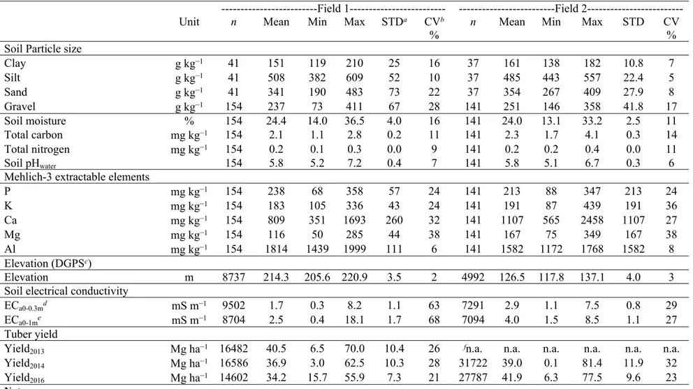
Most soil physicochemical properties had CV values within the range of 5 to 38% for both fields (Table 1). The greatest variability (38%) was obtained for soil Mg content, while the lowest variability was observed for soil Al content and soil pH (6 to 8%). Other studies evaluating spatial variation also found lowest variability for soil pH (Cox et al. 2003; Farooque et al. 2012), which is due to the logarithmic scale of pH measurement.
Overall, Field 1 showed greater variability in soil physical and chemical properties than Field 2. This is probably due to the greatest pedodiversity of Field 1 as suggested by the observed high variation in soil drainage and texture classes of the different soil series (Fig. 1). The CV values of soil texture parameters and soil moisture content were greater in Field 1 than in Field 2. In contrast, soil K content had low and moderate variability in Field 1 and Field 2, respectively. Previous studies evaluating spatial variation reported moderate to high CV values of soil properties (Case 2000; Farooque et al. 2012) in New Brunswick and Nova Scotia, whereas CV values in the current study are generally lower.
The CV values for soil ECa were greater in Field 1 than in Field 2 (Table 1), probably due to the greatest pedodiversity within Field 1, and in particular to greater variability in soil texture and soil moisture content. Tuber yield varied moderately with CV values ranging from 21 to 28% and 23 to 32% for Field 1 and Field 2, respectively (Table 1). Average tuber yield for Field 1 was 40.5 Mg ha–1 in 2013, 36.9 Mg ha–1 in 2014 and 34.2 Mg ha–1 in 2016. The tuber yield variability among years in this field may reflect variation in growing season (May to September) precipitation; growing season
precipitation was 684 mm in 2013, 430 mm in 2014 and 459 mm in 2016 (New Brunswick Government 2016). Similarly for Field 2, greater tuber yield in 2016 over 2014 (41.9 Mg ha–1 vs 39.0 Mg ha–1) is consistent with greater growing season precipitation in 2016 over 2014 (721 mm vs 561 mm) (New Brunswick Government 2016).
Greater within-field variability would require more samples to achieve good prediction accuracy (Nyiraneza et al. 2011). In this study, the moderate variability of the soil physicochemical properties was promising for mapping these agricultural fields. The CV values were generally good indicators of the degree of variability, but not of its nature (i.e., structured or randomized variability; (Cambouris et al. 2006).
Spatial variability
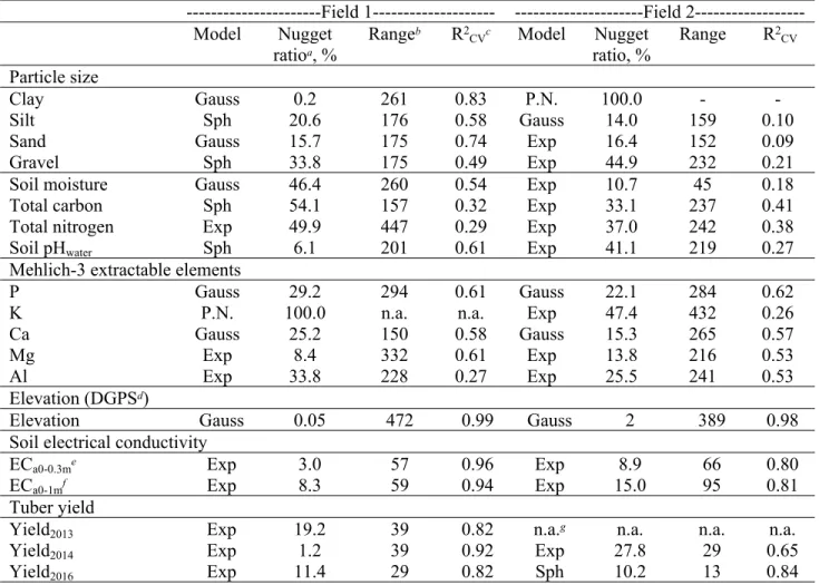
Among the available models for fitting with experimental semivariogram, Gaussian, spherical, and exponential models were the best fit for most of the soil physicochemical properties and elevation in both fields (Table 2). However, the pure nugget models were the best fit for soil K content in Field 1 and clay content in Field 2. The pure nugget effect may be a result of sampling errors, random inherent variability, and/or short-range variability and indicated a complete lack of spatial structure. Spatial ranges for measured soil properties varied from 45 to 447 m. The spatial ranges of the soil properties were greater than the 33 m grid spacing, indicating that the grid sampling intensity used to characterize the spatial variability of both fields was appropriate in this study. Except for the pure nugget semivariogram models, most soil property nugget ratio values indicated moderate to strong spatial dependence.
The best fit semivariogram models for soil ECa and tuber yield were generally exponential and spherical, respectively (Table 2). For soil ECa measurements, the range varied from 57 to 95 m and the nugget ratio was ≤ 15% for both fields (Table 2). This suggested that the nugget effect (random variance) was very low and reliably modelled by the sampling strategies (434 soil ECa measurements per ha–1) (Cambouris et al. 2006; Simard et al. 2001). Similar results were reported by Moral et al. (2010) for soil ECa in silt loam soils from southwestern Spain. The tuber yield nugget ratio varied from 1 to 28% and the spatial range varied from 13 to 39 m for both fields. These results also indicated that soil ECa and tuber yield are strong spatially dependent properties and are probably controlled by intrinsic factors (e.g., soil texture, structure, mineralogy and microorganisms) (Cambardella and Karlen 1999; Cambardella et al. 1994).
High R2CV values (i.e., > 0.60) indicated that good fits were obtained for most of the densely measured properties (i.e., elevation, soil ECa, and tuber yield) for both fields (Table 2). This suggests that these properties can then be used to delineate MZs. Good fit models were also obtained for the soil particle size distribution and soil moisture in Field 1 (R2CV = 0.49 to 0.83), whereas the fit was relatively weaker in Field 2 (R2CV = 0.03 to 0.21). In contrast to Field 2, the R2CV values suggested that the spatial dependence of properties in Field 1 could be influenced mostly by intrinsic soil factors (Cambardella and Karlen 1999).
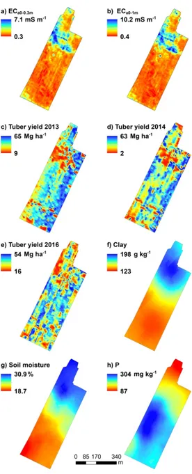
Soil ECa values were generally greatest in the northern part of Field 1, with lower soil ECa values in the central and southern parts of the field (Fig. 2a, b). There was a consistent and constant variability of tuber yield in 2013, 2014 and 2016 in Field 1 (Fig. 2c, d, e). Therefore in Field 1, the within-field variation in yield attributable to spatial
variability in physicochemical properties was greater than induced by seasonal climatic conditions. The spatial variability of clay, soil moisture and P contents showed good visual similitude in Field 1 (Fig. 2f, g, h). Greater clay and soil moisture contents were associated with lower P content. The lowest area of P content could be related to the recent land clearing (<5 yr) and potato cultivation in the northern part of the field. It is known that uniform application of fertilizer in the entire field could also contribute to maintaining this difference (Cambouris et al. 1999).
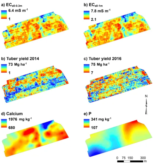
In contrast, soil ECa measurements did not show similar spatial patterns as the soil texture parameters in Field 2 (Fig. 3a, b). The spatial pattern of tuber yield varied between years, indicating the pattern of yield was not temporally stable (Fig. 3b, c).The Ca and the P content maps showed similarities in Field 2, where areas with high Ca content were characterized by low P content (Fig. 3d, e).
Relationships between ECa, soil properties and crop yield
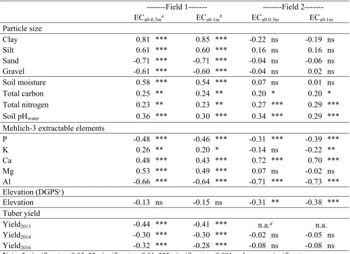
Soil ECa values were strongly correlated with soil texture and soil moisture in Field 1 (Table 3). Soil ECa values, clay and soil moisture contents were greater in the areas characterized by poorly drained soils (Fig. 2a, b, f, g). Previous studies reported similar relationships between soil ECa values and soil texture under similar soil and topographic conditions (Landrum et al. 2015; Moral et al. 2010). Mehlich-3 extractable elements, total carbon and nitrogen and soil pH were also generally significantly correlated with the soil ECa values in Field 1. Overall, the strong correlations of soil properties with soil ECa values suggested that soil ECa can be used to predict the spatial distribution of soil properties, to visualize their impact on crop yield, and ameliorate productive and unproductive areas within a field. Soil ECa measurements were negatively
correlated with tuber yield in 2013, 2014 and 2016 for Field 1 (Table 3). Stronger correlations were obtained in 2013, which may be associated with greater growing season precipitation. The correlation coefficients between soil ECa and tuber yield were similar to those reported by Cambouris et al. (2006) (r = 0.25 to 0.49). Areas of the field with the greatest clay content (Fig. 2f) had the lowest tuber yield (Fig. 2c, d, e). Low yield areas were also characterized by high soil moisture content (Fig. 2g), which indicates poorly drained soil. Potato production is severely impeded due to drainage. For example, healthy root and tuber development can be affected by the free movement of oxygen with excessive water. The surplus of water in soil can also limit the efficiency of nutrient uptake, increase fungal diseases, increase the risk of soil compaction not to mention the delays of spring tillage and planting (New Brunswick Department of Agriculture 2018; Stark et al. 2004). Low yield areas were also characterized by low P content (Fig. 2h), which is essential for root development (Nyiraneza et al. 2017).
In contrast, there is no apparent relationship between soil ECa and soil texture in Field 2 (Table 3). There is, however, a strong correlation between the Mehlich-3 extractable elements (Ca, Al and P) and the soil ECa measurements (Table 3). The area with increased ECa had greater Ca content and lower P and Al contents (Fig. 3). Soil ECa measurements were not related to tuber yield in 2014 or 2016 in Field 2. Significant negative correlations of soil ECa measurements with elevation (Table 3) suggested a linear trend, indicating that the ground conductivity values were strongly influenced by the topography in Field 2. In accordance with previous results, soil ECa showed superior performance in explaining the spatial variability in soil properties in the studied fields, especially for Field 1.
Determination of the optimum number of management zones
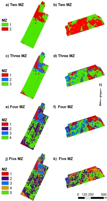
The fuzzy k-means clustering algorithm was used to partition the fields into two to five MZs (Fig. 4). When the analysis was first carried out with a spatial constraint of proximity, the algorithm could not handle the spatial structure, and led to the delineation of artificial regions based only on the numerical values of spatial coordinate and not on the geographical proximity (data not shown). Consequently, the analysis was performed without a spatial constraint of proximity. As expected, increasing the number of MZs from one to five decreased the total within-zone variance of the soil and yield parameters (Cambouris et al. 2006). Similar to previous studies (Li et al. 2007; Moral et al. 2010; Xin-Zhong et al. 2009), the magnitude of the reduction in total within-zone variance was used to select the optimum number of MZs.
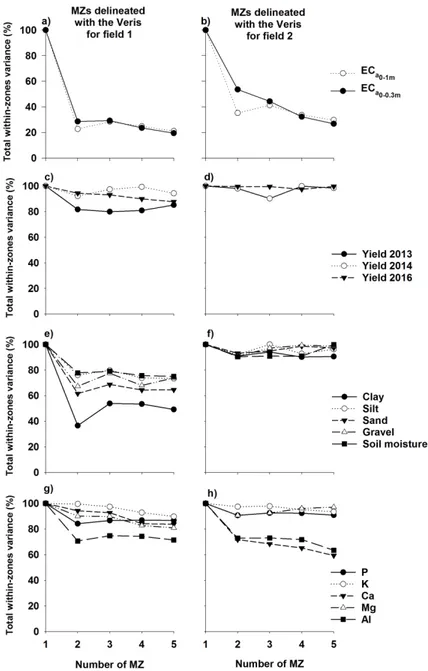
At Field 1, going from one to two MZs decreased total within-zone variance of soil ECa by 71 to 77% (Fig. 5a). This magnitude in the decrease of variance for soil ECa values is comparable with that reported by Cambouris et al. (2006) and Corwin and Lesch (2005). Additional MZs resulted in a limited reduction in total within-zone variance of soil ECa, and consequently two MZs was determined to be most suitable for this field. The decrease in variance for total yield in going from one to two MZs varied among years, with total within-zone variance decreased by 18% in 2013, 8% in 2014 and 6% in 2016 (Fig. 5c). Clay content and soil moisture showed a total variance reduction of 63% and 23%, respectively, with two MZs compared to single zone or whole field as a management unit (Fig. 5e). For soil chemical properties, going to two MZs decreased the total variance for P and Al contents by 19 and 29%, respectively (Fig. 5g). Moral et al.
(2010) also identified two MZs as the optimum number when using electromagnetic induction to classify their field.
At Field 2, going from one to two MZs decreased the total within-zone variance of soil ECa values by 46 to 65% (Fig. 5b). Based on the total yield and most of the physicochemical properties, the subdivision of Field 2 from one to five MZs resulted in a decrease in the total variance of less than 10% (Fig. 5d, f, h). In contrast, going from one to two MZs decreased the total variance of Ca and Al contents by 28 and 27%, respectively (Fig. 5h). For Field 2, the decrease in variance followed a less homogeneous behaviour than in Field 1, and did not show any clear pattern of MZs. This may be attributed to the relatively homogeneous spatial variability and a weaker spatial structure for soil properties in Field 2. Corwin and Lesch (2005) noticed that performance of soil ECa sensors varies from field to field, especially when the field is dominated by one or two intrinsic factors such as soil moisture or clay content which make the interpretation of soil ECa values highly specific to the field.
Practical applications of management zone within these fields
Spatial variability in crops is the result of a complex interaction of biological, edaphic, anthropogenic, topographic, and climatic factors (Corwin and Lesch 2003). Measurements of soil ECa have been used at field scale to map spatial variability of soil properties and yield by MZs. According to Cambouris et al. (2006), the optimal number of MZs must show a balance between the spatial variation of soil properties, yield stability over time and a manageable spatial representation. Analysis of variance was conducted to provide an indication of statistical distinction among different MZs (Chang et al. 2014). In general, three or more MZs were not considered significant at the chosen
5% level (data not shown), and effectively only two MZs were significantly different based on soil ECa values in both fields (Table 4).
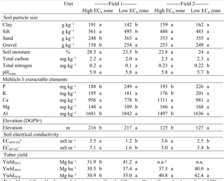
In Field 1, the two MZs delineated using soil ECa measurements differed significantly in tuber yield for all three years and in most of the soil physicochemical properties measured (Table 4). When averaged across the three years, tuber yield was 6.8 Mg ha–1 greater for the low ECa zone than for the high ECa zone. The high ECa zone, which had lower yield, was characterized by greater soil pH and contents of clay, soil moisture, total carbon and nitrogen, Ca and Mg, while it had lower contents of sand, gravel, P and Al. Since the soil physicochemical properties varied significantly between MZs, it may be relevant to manage soil properties using the selected MZs. For example, the high soil ECa zone was characterized by the wettest soil, the finest soil texture and the lowest tuber yield. The wet soil conditions in the high ECa zone could be managed with specific drainage or land levelling to prevent water accumulation, leading to increase in the tuber yield potential. This confirms that by identifying the underlying factors responsible for the variation in crop yield, it may be possible for potato producers to use MZs in order to optimize their profitability (De Caires et al. 2015).
For Field 2, the high ECa MZ had greater soil pH and total N content, and lower contents of P, K, and Al compared with the low ECa MZ (Table 4). In contrast, tuber yield for two years, soil texture, soil moisture, total C and Ca content were not significantly different between MZ. Sim
A site-specific crop management can be implemented in agricultural fields to manage plant breeding, pest management, weed management, soil fertility and crops based upon spatial variations within a field (Khosla et al. 2010). Two MZs could be
determined in both fields; however, only the MZs delineated in Field 1 were related to tuber yield. The zone delineation has the potential to facilitate cost-effective, environmentally friendly and energy efficient management of the fields (De Caires et al. 2015), particularly when the field shows high spatial variability such as in Field 1.
CONCLUSIONS
In this study, soil ECa was effective in delineating within-field differences in soil physicochemical properties in two agricultural fields. Consequently in these fields, soil ECa is an efficient variable to stratify and reduce the within-field soil variability by delineating homogeneous soil MZs on the basis of soil characteristics. The MZs delineated with soil ECa coincided with the spatial variation in tuber yield in Field 1. This field showed high pedodiversity in soil texture and soil moisture, and these properties influenced soil water availability, and consequently potato yield. The spatial distribution of potato tuber yield in Field 1 was also stable over time, and thus could be used for implementing site-specific crop management. In contrast, the spatial distributions of potato tuber yield in Field 2 did not follow the spatial pattern of other soil physiochemical properties measured. However, some soil Mehlich-3 extractable elements (P, K and Al) were significantly different between high and low soil ECa MZs. Soil proximal sensors, such as Veris®, performances to map spatial variability of intrinsic soil properties is promising in potato production in New Brunswick, especially in fields with high pedodiversity.
ACKNOWLEDGMENTS
This project was funded by the AgriInnovation Program of Agriculture and Agri-Food Canada (AAFC). The authors would like to thank Sarah-Maude Parent, Claude Lévesque, Ginette Decker, Kyle MacKinley and Gordon Fairchild (Eastern Canada Soil and Water Conservation Centre) for their field work and laboratory support.
REFERENCES
Adamchuk, V., Allred, B., Doolittle, J., Grote, K. and Rossel, R. 2015. Tools for
proximal soil sensing. Soil Survey Staff, Ditzler, C., West, L.(Eds.), Soil Survey Manual. Natural Resources Conservation Service. US Department of Agriculture Handbook 18.
Adamchuk, V. I., Hummel, J. W., Morgan, M. T. and Upadhyaya, S. K. 2004.
On-the-go soil sensors for precision agriculture. Comput. Electronics in Agric. 44(1): 71–91. doi: http://dx.doi.org/10.1016/j.compag.2004.03.002.
Agriculture and Agri-Food Canada. 2017. Potato market information review. [Online]
Available:
http://www.agr.gc.ca/resources/prod/doc/pdf/potato_market_review_revue_march e_pomme_terre_2016a-eng.pdf [16-05, 2018].
Allaire, S. E., Baril, B., Vanasse, A., Lange, S. F., MacKay, J. and Smith, D. L. 2014.
Carbon dynamics in a biochar-amended loamy soil under switchgrass. Can. J. Soil Sci.: 1–13. doi: 10.4141/cjss-2014-042.
Cambardella, C. A. and Karlen, D. L. 1999. Spatial Analysis of Soil Fertility
Parameters. Precis. Agric. 1(1): 5–14. doi: 10.1023/A:1009925919134.
Cambardella, C. A., Moorman, T. B., Parkin, T. B., Karlen, D. L., Novak, J. M., Turco, R. F. and Konopka, A. E. 1994. Field-scale variability of soil properties
in central Iowa soils. Soil Sci. Soc. Am. J. 58(5): 1501–1511.
Cambouris, A. N., Nolin, M. C. and Simard, R. R. 1999. Precision management of
fertilizer phosphorus and potassium for potato in Quebec, Canada. Precis. Agric.(precisionagric4a): 847-857.
Cambouris, A. N., Nolin, M. C., Zebarth, B. J. and Laverdière, M. R. 2006. Soil
management zones delineated by electrical conductivity to characterize spatial and temporal variations in potato yield and in soil properties. Am. J. Potato Res.
83(5): 381–395. doi: 10.1007/BF02872015.
Cambouris, A. N., Zebarth, B. J., Ziadi, N. and Perron, I. 2014. Precision Agriculture
in Potato Production. Potato Research: 1–14. doi: 10.1007/s11540-014-9266-0.
Canadian Potato Council. 2016. National Research and Innovation Strategy. [Online]
Available: https://hortcouncil.ca/wp-content/uploads/2017/05/2016-Updated-CPC-National-Research-Strategy-FINAL_En.pdf.
Case, B. S. 2000. Interpreting the spatial distribution of select soil properties in two New
Brunswick upland watersheds by way of the flow accumulation concept. University of New Brunswick. 143 pp.
Chang, D., Zhang, J., Zhu, L., Ge, S.-H., Li, P.-Y. and Liu, G.-S. 2014. Delineation of
management zones using an active canopy sensor for a tobacco field. Comput.
Electronics in Agric. 109(0): 172–178. doi:
http://dx.doi.org/10.1016/j.compag.2014.09.019.
Corwin, D. L. and Lesch, S. M. 2003. Application of soil electrical conductivity to
precision agriculture. Agron. J. 95(3): 455–471. doi: 10.2134/agronj2003.4550.
Corwin, D. L. and Lesch, S. M. 2005. Apparent soil electrical conductivity
measurements in agriculture. Comput. Electronics in Agric. 46(1/3): 11–43. doi:
http://dx.doi.org/10.1016/j.compag.2004.10.005.
Corwin, D. L. and Lesch, S. M. 2010. Delineating Site-Specific Management Units with
Proximal Sensors. Pages 139–165 in M. A. Oliver, ed. Geostatistical Applications for Precision Agriculture. Springer Netherlands, Dordrecht.
Cox, M., Gerard, P., Wardlaw, M. and Abshire, M. 2003. Variability of selected soil
properties and their relationships with soybean yield. Soil Sci. Soc. Am. J. 67(4): 1296–1302. doi: 10.2136/sssaj2003.1296.
De Caires, S. A., Wuddivira, M. N. and Bekele, I. 2015. Spatial analysis for
management zone delineation in a humid tropic cocoa plantation. Precis. Agric.
16(2): 129–147. doi: 10.1007/s11119-014-9366-5.
Environment Canada. 2016. Canadian Climate Normals, 1981-2010 Climate Normals
& Averages. [Online] Available: http://climate.weather.gc.ca/climate_normals/
[September 26, 2016].
Fahmy, S. H. and Rees, H. W. 1996. Soils of the Woodstock–Florenceville area,
Carleton County, New Brunswick. Research Branch, Agriculture and Agri-Food Canada, Ottawa, ON.
Farooque, A. A., Zaman, Q. U., Schumann, A. W., Madani, A. and Percival, D. C. 2012. Delineating management zones for site specific fertilization in wild
blueberry fields. Applied Engineering in Agriculture 28(1): 57–70.
Hendershot, W. H., Lalande, H. and Duquette, M. 2008. Soil reaction and
exchangeable acidity. Pages 173–178 in R. Carter, E. G. Gregorich, eds. Soil sampling and methods of analysis. Taylor & Francis, Boca Raton, FL.
Khosla, R., Westfall, D. G., Reich, R. M., Mahal, J. S. and Gangloff, W. J. 2010.
Spatial variation and site-specific management zones. Pages 195–219 in M. A. Oliver, ed. Geostatistical Applications for Precision Agriculture. Springer Netherlands, Dordrecht.
Kravchenko, A. N., Bollero, G. A., Omonode, R. A. and Bullock, D. G. 2002.
Quantitative mapping of soil drainage classes using topographical data and soil electrical conductivity. Soil Sci. Soc. Am. J. 66(1): 235–243. doi:
Kroetsch, D. and Wang, C. 2008. Particle size distribution. Pages 713–725 in R. Carter,
E. G. Gregorich, eds. Soil sampling and methods of analysis. Taylor & Francis, Boca Raton, FL.
Kweon, G., Lund, E. and Maxton, C. 2012. The ultimate soil survey in one pass: soil
texture, organic matter, ph, elevation, slope, and curvature. Proc. 11th International Conference on Precision Agriculture.
Landrum, C., Castrignanò, A., Mueller, T., Zourarakis, D., Zhu, J. and De Benedetto, D. 2015. An approach for delineating homogeneous within-field
zones using proximal sensing and multivariate geostatistics. Agric. Water Manage. 147: 144–153. doi: http://dx.doi.org/10.1016/j.agwat.2014.07.013.
Langmaid, K., MacMillan, J. and Losier, J. 1980. Soils of Madawaska County. New
Brunswick. Res. Branch, Canada Dep. of Agric. and New Brunswick Dep. of Agric., Fredericton, NB.
Li, Y., Shi, Z., Li, F. and Li, H.-Y. 2007. Delineation of site-specific management zones
using fuzzy clustering analysis in a coastal saline land. Comput. Electronics in Agric. 56(2): 174–186. doi: https://doi.org/10.1016/j.compag.2007.01.013.
McBratney, A. B. 1992. On variation, uncertainty and informatics in environmental soil
management. Soil Research 30(6): 913-935. doi:
https://doi.org/10.1071/SR9920913.
McBratney, A. B. and de Gruijter, J. J. 1992. A continuum approach to soil
classification by modified fuzzy k-means with extragrades. Journal of Soil Science 43(1): 159–175. doi: 10.1111/j.1365-2389.1992.tb00127.x.
Milburn, P., Rees, H., Fahmy, S. and Gartley, C. 1989. Soil depth groups for
agricultural land development planning in New Brunswick. Can. Agric. Eng 31: 1–5.
Minasny, B. and McBratney, A. 2002. FuzME version 3.0. Australian Centre for
Precision Agriculture, The University of Sydney, Australia.
Moral, F. J., Terrón, J. M. and Silva, J. R. M. d. 2010. Delineation of management
zones using mobile measurements of soil apparent electrical conductivity and multivariate geostatistical techniques. Soil & Tillage Res. 106(2): 335–343. doi:
https://doi.org/10.1016/j.still.2009.12.002.
Morier, T., Cambouris, A. N. and Chokmani, K. 2015. In-Season Nitrogen Status
Assessment and Yield Estimation Using Hyperspectral Vegetation Indices in a Potato Crop. Agron. J. 107(4): 1295–1309. doi: 10.2134/agronj14.0402.
Mueller, T. G., Hartsock, N. J., Stombaugh, T. S., Shearer, S. A., Cornelius, P. L. and Barnhisel, R. I. 2003. Soil Electrical Conductivity Map Variability in
Limestone Soils Overlain by Loess Contrib. no. 01-06-61 from the Kentucky Agric. Exp. Stn., Lexington, KY. Agron. J. 95(3): 496–507. doi: 10.2134/agronj2003.4960.
Mulla, D. 1989. Soil spatial variability and methods of analysis. Proc. International
Workshop on Soil, Crop, and Water Management Systems for Rainfed Agriculture in the Sudano-Sahelian Zone, Niamey (Niger), 11-16 Jan 1987.
New Brunswick Department of Agriculture, Aquaculture and Fisheries,,. 2018.
Potatoes soil management. [Online] Available:
http://www2.gnb.ca/content/gnb/en/departments/10/agriculture/content/crops/pota toes/soil_management.html [4 September, 2018].
New Brunswick Government. 2001. Guide de fertilisation des cultures. Pages 34.
New Brunswick Government. 2016. Potato Crop Update. [Online] Available:
http://www2.gnb.ca/content/gnb/en/departments/10/agriculture/content/crop_upda tes/2016.html [December, 11, 2017].
Nyiraneza, J., Bizimungu, B., Messiga, A. J., Fuller, K. D., Fillmore, S. A. E. and Jiang, Y. 2017. Potato yield and phosphorus use efficiency of two new potato
cultivars in New Brunswick, Canada. Can. J. Plant Sci. 97(5): 784–795. doi: 10.1139/cjps-2016-0330.
Nyiraneza, J., Nolin, M. C., Ziadi, N. and Cambouris, A. N. 2011. Short-range
variability of nitrate and phosphate desorbed from anionic exchange membranes. Soil Sci. Soc. Am. J. 75(6): 2242–2250. doi: 10.2136/sssaj2011.0141.
Peralta, N. R. and Costa, J. L. 2013. Delineation of management zones with soil
apparent electrical conductivity to improve nutrient management. Comput. Electronics in Agric. 99: 218–226. doi: 10.1016/j.compag.2013.09.014.
Peralta, N. R., Costa, J. L., Balzarini, M., Castro Franco, M., Córdoba, M. and Bullock, D. 2015. Delineation of management zones to improve nitrogen
management of wheat. Comput. Electronics in Agric. 110: 103–113. doi:
https://doi.org/10.1016/j.compag.2014.10.017.
Sanches, G. M., Magalhães, P. S. G., Remacre, A. Z. and Franco, H. C. J. 2018.
Potential of apparent soil electrical conductivity to describe the soil pH and improve lime application in a clayey soil. Soil & Tillage Res. 175: 217–225. doi: 10.1016/j.still.2017.09.010.
Shaner, D. L., Khosla, R., Brodahl, M. K., Buchleiter, G. W. and Farahani, H. J. 2008. How Well Does Zone Sampling Based on Soil Electrical Conductivity
Maps Represent Soil Variability? Agron. J. 100(5): 1472–1480. doi: 10.2134/agronj2008.0060.
Simard, R. R., Ziadi, N., Nolin, M. C. and Cambouris, A. N. 2001. Prediction of
nitrogen responses of corn by soil nitrogen mineralization indicators. The Scientific World 1 Suppl 2: 135–41. doi: 10.1100/tsw.2001.329.
Stark, J., Westermann, D. and Hopkins, B. 2004. Nutrient Management Guidelines for
Russet Burbank Potatoes. Pages 12. University of Idaho.
Sudduth, K. A., Drummond, S. T. and Kitchen, N. R. 2001. Accuracy issues in
electromagnetic induction sensing of soil electrical conductivity for precision
agriculture. Comput. Electronics in Agric. 31(3): 239–264. doi:
https://doi.org/10.1016/S0168-1699(00)00185-X.
Sudduth, K. A., Kitchen, N. R., Bollero, G. A., Bullock, D. G. and Wiebold, W. J. 2003. Comparison of Electromagnetic Induction and Direct Sensing of Soil
Electrical Conductivity. Agron. J. 95(3): 472–482. doi: 10.2134/agronj2003.4720.
Toy, C. W., Steelman, C. M. and Endres, A. L. 2010. Comparing electromagnetic
induction and ground penetrating radar techniques for estimating soil moisture content. Proc. 13th International Conference on Ground Penetrating Radar.
Tripathi, R., Nayak, A. K., Shahid, M., Lal, B., Gautam, P., Raja, R., Mohanty, S., Kumar, A., Panda, B. B. and Sahoo, R. N. 2015. Delineation of soil
management zones for a rice cultivated area in eastern India using fuzzy clustering. CATENA 133: 128–136. doi: 10.1016/j.catena.2015.05.009.
Wu, C., Wu, J., Luo, Y., Zhang, L. and DeGloria, S. D. 2009. Spatial prediction of soil
organic matter content using cokriging with remotely sensed data. Soil Sci. Soc. Am. J. 73(4): 1202–1208. doi: 10.2136/sssaj2008.0045.
Xin-Zhong, W., Guo-Shun, L., Hong-Chao, H., Zhen-Hai, W., Qing-Hua, L., Xu-Feng, L., Wei-Hong, H. and Yan-Tao, L. 2009. Determination of management
zones for a tobacco field based on soil fertility. Comput. Electronics in Agric.
65(2): 168–175. doi: https://doi.org/10.1016/j.compag.2008.08.008.
Ziadi, N. and Tran, T. 2008. Mehlich 3-Extractable Elements. Pages 81-88 in R. Carter,
E. G. Gregorich, eds. Soil Sampling and Methods of Analysis, Second Edition. Taylor & Francis, Boca Raton, FL.
Fig. 1. Soil series, drainage classes and sampling grid at a) Field 1 and b) Field 2.
Fig. 2. Kriging maps of the apparent soil electrical conductivity (ECa) measured a) ECa0-0.3m and b) ECa0-1m; tuber yield c) 2013, d) 2014 and e) 2016; and f) clay, g) soil moisture and h) Mehlich-3 extractable P of Field 1.
Fig. 3. Kriging maps of the apparent soil electrical conductivity (ECa) a) ECa0-0.3m and b) ECa0-1m; tuber yield c) 2014, and d) 2016; and Mehlich-3 extractable e) Ca and f) P of Field 2.
Fig. 4. Management zones (MZs) delineated using the ECa0-0.3m and ECa0-1m kriged data matrix with the fuzzy k-means analysis with no-spatial constraint of proximity at Field 1 (a-c-e-j) and Field 2 (b-d-f-k).
Fig. 5. Decrease of the total within-zone variance of a-b) soil electrical conductivity, c-d) yields 2013, 2014 and 2016 from yield monitor, e-f) soil particles sizes (clay, silt, sand), gravel and soil moisture, g-h) Mehlich-3 extractable elements (P, K, Ca, Mg and Al) into management zone (MZs) based on the MZs delineated with the Veris® at Field 1 and Field 2, respectively.
26
Table 1. Descriptive statistics of the soil physicochemical properties, elevation, soil electrical conductivity and tuber yield for Field 1 and Field 2
---Field 1--- ---Field
2---Unit n Mean Min Max STDa CVb
%
n Mean Min Max STD CV
% Soil Particle size
Clay g kg–1 41 151 119 210 25 16 37 161 138 182 10.8 7 Silt g kg–1 41 508 382 609 52 10 37 485 443 557 22.4 5 Sand g kg–1 41 341 190 483 73 22 37 354 267 409 27.9 8 Gravel g kg–1 154 237 73 411 67 28 141 251 146 358 41.8 17 Soil moisture % 154 24.4 14.0 36.5 4.0 16 141 24.0 13.1 33.2 2.5 11 Total carbon mg kg–1 154 2.1 1.1 2.8 0.2 11 141 2.3 1.7 4.1 0.3 14 Total nitrogen mg kg–1 154 0.2 0.1 0.3 0.0 9 141 0.2 0.2 0.4 0.0 11 Soil pHwater 154 5.8 5.2 7.2 0.4 7 141 5.8 5.1 6.7 0.3 6
Mehlich-3 extractable elements
P mg kg–1 154 238 68 358 57 24 141 213 88 347 213 24 K mg kg–1 154 183 105 336 43 24 141 191 87 439 191 36 Ca mg kg–1 154 809 351 1693 260 32 141 1107 565 2458 1107 27 Mg mg kg–1 154 116 50 285 44 38 141 167 75 349 167 38 Al mg kg–1 154 1814 1439 1999 111 6 141 1582 1172 1768 1582 8 Elevation (DGPSc) Elevation m 8737 214.3 205.6 220.9 3.5 2 4992 126.5 117.8 137.1 4.0 3
Soil electrical conductivity
ECa0-0.3md mS m–1 9502 1.7 0.3 8.2 1.1 63 7291 2.9 1.1 7.5 0.8 29
ECa0-1me mS m–1 8704 2.5 0.4 18.1 1.7 68 7094 4.0 1.5 8.5 1.1 27
Tuber yield
Yield2013 Mg ha–1 16482 40.5 6.5 70.0 10.4 26 fn.a. n.a. n.a. n.a. n.a. n.a.
Yield2014 Mg ha–1 16586 36.9 3.0 62.5 10.3 28 31722 39.0 0.1 81.4 11.9 32
Yield2016 Mg ha–1 14602 34.2 15.7 55.9 7.3 21 27787 41.9 6.3 77.5 9.6 23
Note:
aSTD, standard deviation,
27 bCV, coefficient of variation;
cDGPS, differential global positioning system; dEC
a0-0.3m, shallow measurements of soil ECa measured at 0-0.3 m; eEC
a0-1m, deep measurements of soil ECa measured at 0-1.0 m; fn.a., not available.
Table 2. Geostatistical parameters of the soil physicochemical properties for Field 1 and Field 2 ---Field 1--- ---Field 2---Model Nugget ratioa, % Rangeb R2 CVc Model Nugget ratio, % Range R2 CV Particle size Clay Gauss 0.2 261 0.83 P.N. 100.0 - -Silt Sph 20.6 176 0.58 Gauss 14.0 159 0.10
Sand Gauss 15.7 175 0.74 Exp 16.4 152 0.09
Gravel Sph 33.8 175 0.49 Exp 44.9 232 0.21
Soil moisture Gauss 46.4 260 0.54 Exp 10.7 45 0.18
Total carbon Sph 54.1 157 0.32 Exp 33.1 237 0.41
Total nitrogen Exp 49.9 447 0.29 Exp 37.0 242 0.38
Soil pHwater Sph 6.1 201 0.61 Exp 41.1 219 0.27
Mehlich-3 extractable elements
P Gauss 29.2 294 0.61 Gauss 22.1 284 0.62
K P.N. 100.0 n.a. n.a. Exp 47.4 432 0.26
Ca Gauss 25.2 150 0.58 Gauss 15.3 265 0.57
Mg Exp 8.4 332 0.61 Exp 13.8 216 0.53
Al Exp 33.8 228 0.27 Exp 25.5 241 0.53
Elevation (DGPSd)
Elevation Gauss 0.05 472 0.99 Gauss 2 389 0.98
Soil electrical conductivity
ECa0-0.3me Exp 3.0 57 0.96 Exp 8.9 66 0.80
ECa0-1mf Exp 8.3 59 0.94 Exp 15.0 95 0.81
Tuber yield
Yield2013 Exp 19.2 39 0.82 n.a.g n.a. n.a. n.a.
Yield2014 Exp 1.2 39 0.92 Exp 27.8 29 0.65
Yield2016 Exp 11.4 29 0.82 Sph 10.2 13 0.84
Note: Gauss, Gaussian; Sph, spherical; Exp, exponential; P.N., pure nugget; aNugget ratio, (nugget semivariance/total semivariance) × 100;
bRange, distance at which a semivariance becomes constant; cR2
CV,coefficient of determination of cross-validation; dDGPS, differential global positioning system; eEC
a0-0.3m, shallow measurements of soil ECa measured at 0-0.3 m; fEC
a0-1m, deep measurements of soil ECa measured at 0-1.0 m; gn.a., not available.
Table 3. Pearson correlation coefficients (r) of the soil electrical conductivity (Veris®) with soil properties, elevation (DGPS) and tuber yield (yield monitor) at Field 1 and Field 2
---Field 1--- ---Field
2---ECa0-0.3ma ECa0-1mb ECa0-0.3m ECa0-1m
Particle size Clay 0.81 *** 0.85 *** -0.22 ns -0.19 ns Silt 0.61 *** 0.60 *** 0.16 ns 0.16 ns Sand -0.71 *** -0.71 *** -0.04 ns -0.06 ns Gravel -0.61 *** -0.60 *** -0.04 ns 0.02 ns Soil moisture 0.58 *** 0.54 *** 0.07 ns 0.01 ns Total carbon 0.25 ** 0.24 ** 0.20 * 0.20 * Total nitrogen 0.23 ** 0.23 ** 0.27 *** 0.29 *** Soil pHwater 0.36 *** 0.30 *** 0.34 *** 0.29 ***
Mehlich-3 extractable elements
P -0.48 *** -0.46 *** -0.31 *** -0.39 *** K 0.26 ** 0.20 * -0.14 ns -0.22 ** Ca 0.48 *** 0.43 *** 0.72 *** 0.70 *** Mg 0.53 *** 0.49 *** 0.07 ns -0.02 ns Al -0.66 *** -0.64 *** -0.71 *** -0.73 *** Elevation (DGPSc) Elevation -0.13 ns -0.15 ns -0.31 ** -0.38 *** Tuber yield
Yield2013 -0.44 *** -0.41 *** n.a.d n.a.
Yield2014 -0.30 *** -0.30 *** -0.02 ns -0.05 ns
Yield2016 -0.32 *** -0.28 *** -0.08 ns -0.08 ns
Note: *, significant ρ <0.05; **, significant ρ <0.01; ***, significant ρ <0.001 and ns, non-significant aEC
a0-0.3m, shallow measurements of soil ECa measured at 0-0.3 m; bEC
a0-1m, deep measurements of soil ECa measured at 0-1.0 m; cDGPS, differential global positioning system;
dn.a., not available.
Table 4. Comparison of soil electrical conductivity (ECa) into two management zones at Field 1 and Field 2
Unit ---Field 1--- ---Field
2---High ECa zone Low ECa zone High ECa zone Low ECa zone
Soil particle size
Clay g kg–1 191 a 142 b 159 a 162 a Silt g kg–1 561 a 495 b 488 a 483 a Sand g kg–1 248 b 363 a 353 a 355 a Gravel g kg–1 158 b 254 a 253 a 249 a Soil moisture % 28.5 a 23.5 b 23.8 a 24 a Total carbon mg kg–1 2.2 a 2.0 a 2.3 a 2.3 a Total nitrogen mg kg–1 0.2 a 0.1 a 0.23 a 0.22 b pHwater 5.9 a 5.8 a 5.8 a 5.7 b
Mehlich-3 extractable elements
P mg kg–1 188 b 249 a 193 b 226 a K mg kg–1 195 a 181 a 176 b 201 a Ca mg kg–1 956 a 778 b 1311 a 981 a Mg mg kg–1 148 a 109 b 166 a 168 a Al mg kg–1 1681 b 1842 a 1497 b 1636 a Elevation (DGPSa) Elevation m 216 b 217 a 125 b 127 a
Soil electrical conductivity
ECa0-0.3mb mS m–1 3.5 a 1.2 b 3.6 a 2.5 b
ECa0-1mc mS m–1 5.1 a 1.6 b 5.0 a 3.4 b
Tuber yield
Yield2013 Mg ha–1 31.9 b 41.2 a n.a.d n.a.
Yield2014 Mg ha–1 30.5 b 37.4 a 37.3 a 40.0 a
Yield2016 Mg ha–1 30.9 b 35.0 a 40.8 a 42.4 a
Note: Means followed by the same letter are not significantly different at 5% significance level according to LSD
test;
aDGPS, differential global positioning system; bEC
a0-0.3m, shallow measurements of soil ECa measured at 0-0.3 m; cECa0-1m, deep measurements of soil ECa measured at 0-1.0 m. dn.a., not available.
Fig. 2. Kriging maps of the apparent soil electrical conductivity (ECa) measured a) ECa0-0.3m and b) EC
a0-1m; tuber yield c) 2013, d) 2014 and e) 2016; and f) clay, g) soil moisture and h) Mehlich-3 extractable P of
Field 1.
254x558mm (300 x 300 DPI)
Fig. 3. Kriging maps of the apparent soil electrical conductivity (ECa) a) ECa0-0.3m and b) ECa0-1m; tuber yield c) 2014, and d) 2016; and Mehlich-3 extractable e) Ca and f) P of Field 2.
431x431mm (300 x 300 DPI)
Fig. 4. Management zones (MZs) delineated using the Veris® ECa0-0.3m and ECa0-1m kriged data matrix with the fuzzy k-means analysis with no-spatial constraint of proximity at the field 1 (a-c-e-j) and field 2
(b-d-f-k).
431x667mm (300 x 300 DPI)
Fig 5. Decrease of the total within-zone variance of a-b) soil electrical conductivity using the Veris®, c-d) yields 2013, 2014 and 2016 from yield monitor, e-f) soil particles sizes (clay, silt, sand), gravel and soil moisture, g-h) Mehlich-3 extractable elements (P, K, Ca, Mg and Al) into management zone (MZs) based on
the MZs delineated with the Veris® at the field 1 and field 2, respectively. 215x278mm (300 x 300 DPI)