Empirical Assessment of an Intertemporal
Option Pricing Model with Latent Variables
René Garcia
Université de Montréal (CIRANO and CRDE) Bank of CanadaRichard Luger Éric Renault
Université de Montréal (CIRANO and CRDE) and CREST-Insee First version: September 2000
This version: February 2002
Abstract
This paper assesses the empirical performance of an intertemporal option pricing model with latent variables which generalizes the Black-Scholes and the stochastic volatility formulas. We derive a closed-form formula for an equilibrium model with recursive preferences where the fundamentals follow a Markov switching process. In a simulation experiment based on the model, we show that option prices are more informative about preference parameters than stock returns. When we estimate the preference parameters implicit in S&P 500 call option prices given our model, we …nd quite reasonable values for the coe¢cient of relative risk aversion and the intertemporal elasticity of substitution.
Keywords: Option Pricing, Stochastic Discount Factor, Stochastic Volatility, Black-Scholes Im-plied Volatility, Smile E¤ect, Equilibrium Option Pricing, Recursive Utility.
JEL Classi…cation: C1,C5,G1
Address for correspondence: René Garcia, Département de Sciences Économiques, Univer-sité de Montréal, C.P. 6128, Succ. Centre-Ville, Montréal, Québec, H3C 3J7, Canada. Tele-phone: (514) 343-5960, fax: (514) 343-5831, email: rene.garcia@umontreal.ca.
1. Introduction
The empirical option pricing literature has revealed a considerable divergence be-tween the risk-neutral distributions estimated from option prices after the 1987 crash and conditional distributions estimated from time series of returns on the underlying index. Three facts come out clearly. First, the implied volatility ex-tracted from at-the-money options di¤ers substantially from the realized volatility over the lifetime of the option. Second, risk neutral distributions feature a sub-stantial negative skewness which is revealed by the asymmetric implied volatility curves when plotted against moneyness. Third, the shape of these volatility curves changes over time, in other words the skewness is time-varying.1
One possible explanation for the divergence between the objective and the risk neutral distributions is the existence of time-varying risk premia. Pan (2002) estimates a jump-di¤usion model proposed by Bates (2000) and investigates how volatility and jump risks are priced in S&P 500 index options. Based on a joint time series of the spot price and of one at-the-money option, Pan (2002) shows that the addition of both volatility and jump risk premia allows to …t well the joint time series of spot and option price data. The model can explain well the changing shapes of the implied volatility curves over time and the skewed pat-terns are largely due to investors’ aversion to jump risks. However, it is not clear how this non-arbitrage continuous-time model relates to the preferences of a representative agent since in this approach investors may have di¤erent risk at-titudes towards the di¤usive return shocks, volatility shocks and jump risks. In a nonparametric framework, Aït-Sahalia and Lo (2000) and Jackwerth (2000) un-cover the risk-aversion function implied by the comparison between the objective and the risk-neutral distributions, while Rosenberg and Engle (2002) investigate the empirical characteristics of investor risk aversion by estimating a daily semi-parametric pricing kernel. Jackwerth (2000) …nds that the preferences are oddly shaped, with marginal utilities increasing for some wealth levels. However, the implied-tree and the kernel methodologies used to recover the risk-neutral and the subjective probabilities are not likely to separate neatly the preferences from the probabilities, especially if the stochastic discount factor depends on state vari-ables. These results underline the potential importance of investors’ preferences
1These facts come out of a string of studies by Bakshi, Cao and Chen (1997), Bates (1996,
for option prices but leave the question of knowing if option prices are compatible with reasonable preferences largely unanswered.
In this paper, we propose a utility-based option pricing model with stochastic volatility and jump features to better understand the relationships between the preferences embedded in risk premia and the aforementioned empirical facts. The model is cast within the recursive utility framework of Epstein and Zin (1989) in which the respective roles of discounting, risk aversion and intertemporal substi-tution are disentangled. This separation might be important for option pricing since an option contract will naturally be a¤ected by the value of time as well as the price of risk associated with the underlying asset. We derive an option pricing formula which generalizes the Black and Scholes (1973) and the Hull and White (1987) and Heston (1993) stochastic volatility formulas, hereafter referred to as BS and SV formulas.2
An essential feature of this generalized option pricing formula is that it is not in general preference-free. In so-called preference-free formulas of which BS and SV are examples, it happens that these parameters are eliminated from the option pricing formula through the observation of the bond price and the stock price. In other words, preference parameters are hidden in the observed stock and bond prices. In our case, the bond pricing formula and the stock pricing formula provide two dynamic restrictions relating the characteristics of the stochastic dis-count factor of the model (which include the preferences) to the bond and stock price processes. The key assumption underlying this result is the presence of an unobserved state variable driving the fundamentals (consumption and dividends) of the economy as in Cecchetti, Lam and Mark (1990, 1993) and Bonomo and Garcia (1994a, 1994b, 1996). This state variable captures the states of the econ-omy which are typically represented by a low consumption growth associated with a high volatility of dividend growth or by a high consumption growth together with a low volatility of dividend growth. A contemporaneous correlation between the state variable and the fundamentals makes the preference parameters play an additional role over and above their impact on stock and bond prices. Therefore, it appears natural to investigate the informativeness of option prices about
pref-2Our formula can be seen as a discrete-time Heston-type formula. However, in contrast with
Heston, the risk premia are explicitly linked to the preference parameters of a representative agent.
erence parameters and to con…rm the dependence of option prices on preference parameters.
First, based on simulations, we show that option prices are more informative than stock returns about the structural parameters of the asset pricing model. More precisely, we show that a set moment conditions based on the mean, vari-ance and autocovarivari-ance of order one of stock returns does not provide good estimates of the preference parameters in …nite samples. Therefore, one can pos-sibly question the empirical tests of intertemporal asset pricing models that have been based mostly on bond and stock returns. On the other hand, similar moment conditions with option prices recover with great accuracy the preference parame-ters. Part of the explanation lies probably in the better spanning of the stochastic discount factor (or the underlying risk neutral probability distribution) by a panel of option prices. The nonlinear nature of the option payo¤s could also help given the nonlinearity in parameters of the model.
We further show that a simple method of moments with a panel of simulated option prices provides good estimates of all the parameters of the model, that is, parameters associated with the fundamentals in the economy along with the preference parameters. This lays the ground for an empirical assessment of the model with S&P 500 option prices in terms of out-of-sample pricing errors and a comparison with usual stochastic volatility and expected utility models which appear as particular cases of our general framework. Our results indicate clearly that the explicit incorporation of preferences improves the performance of the option pricing model and that time non-separable preferences improve the results further. Preference parameter estimates appear reasonable and stable over a …ve-year period (1991-1995).
Apart from the economic interest of recovering preference parameters from this new option pricing formula, there is always the question of its practical use say for forecasting the price of other options. Taking options of all moneyness and all maturities at once, we con…rm that the absolute and relative errors of the non-expected utility model are lower than the errors produced by the expected utility model and a stochastic volatility model. However, the magnitude of the errors remains very large with respect to the errors associated with practitioners’ ad hoc approaches such as plugging in the BS formula implied volatilities of the day or the week before. To put the model on a level playing …eld with ad hoc approaches, we separate the options according to maturity for estimation, we
reduce the period over which empirical moments are computed to the last …ve days and …nally we introduce conditioning information in the estimation. The volatility of the dividend growth is made a function of the implied volatility of the same class of moneyness the day before. This has the e¤ect of reducing the errors to levels more in line with the practitioners’ ad hoc approaches, but given the complex structure of our model, it does not appear as a practical substitute to the simple practitioners’ Black-Scholes. Moreover, this shorter-term calibration blurs the distinctions between the expected utility and the non-expected utility models since they perform quite similarly in terms of predictive ability.
The interplay between preferences and latent factors that a¤ect the stochastic discount factor has been explored to a certain extent in the literature. Amin and Ng (1993) provide an extension of the equilibrium model of Rubinstein (1976) and Brennan (1979) with a systematic stochastic volatility in stock returns. Garcia, Luger and Renault (2001) show that the option pricing model we estimate in this paper can reproduce the various patterns observed in implied volatility curves as well as changing skewness over time. David and Veronesi (1999) show that option prices are a¤ected by investors’ beliefs about the drift of a …rm’s fundamentals. In particular, they emphasize how investors’ beliefs and their degree of risk aversion a¤ect stock returns and hence option prices. Guidolin and Timmermann (1999) explain the empirical biases of the Black-Scholes option pricing model by Bayesian learning e¤ects. The importance of preference parameters in explaining ‡uctua-tions in equity prices has also been explored by Mehra and Sah (1998) who show that small changes in investors’ subjective discount factors and attitudes towards risk can induce volatility in equity prices. The main thesis of the paper is that some instantaneous causality e¤ects between state variables and asset prices can capture the stylized facts of interest without having to introduce any ‡uctuation in beliefs or preferences or learning.
The rest of the paper is organized as follows. Section 2 develops a gener-alized option pricing formula with latent variables based on a recursive utility consumption-based asset pricing model. Section 3 explores, in a simulation ex-periment, the information about preference parameters contained in option prices compared with that in stock returns. Preference parameters are also estimated us-ing S&P 500 option and stock prices. Section 4 calibrates the model for practical option pricing. Section 5 concludes.
2. An Intertemporal Option Pricing Model with Latent Variables We adopt the recursive utility framework proposed by Epstein and Zin (1989). Many identical in…nitely lived agents maximize their lifetime utility and receive each period an endowment of a single nonstorable good. Their recursive utility function is of the form:
Vt = W (Ct; ¹t); (2.1)
where W is an aggregator function that combines current consumption Ct with ¹t = ¹(eVt+1j Jt), a certainty equivalent of random future utility eVt+1; given Jtthe information available to the agents at time t, to obtain the current-period lifetime utility Vt. Following Kreps and Porteus (1978), Epstein and Zin (1989) propose the CES function as the aggregator function, i.e.,
Vt= [Ct½+ ¯¹½t] 1
½: (2.2)
The way the agents form the certainty equivalent of random future utility is based on their risk preferences, which are assumed to be isoelastic, i.e., ¹®
t = E[ eVt+1® jJt]; where ® · 1 is the risk aversion parameter (1-® is the Arrow-Pratt measure of relative risk aversion). Given these preferences, the following Euler condition must be valid for any asset j if an agent maximizes his lifetime utility (see Epstein and Zin 1989):
E[¯°(Ct+1 Ct
)°(½¡1)Mt+1°¡1Rj;t+1jJt] = 1; (2.3) where Mt+1represents the return on the market portfolio, Rj;t+1 the return on any asset j, and ° = ®
½. The parameter ½ is associated with intertemporal substitution, since the elasticity of intertemporal substitution is 1=(1 ¡ ½): The position of ® with respect to ½ determines whether the agent has a preference towards early resolution of uncertainty (® < ½) or late resolution of uncertainty (® > ½).
Since the market portfolio price, say PM
t at time t, is determined in equilibrium, it should also verify the …rst-order condition:
E[¯°(Ct+1 Ct
)°(½¡1)Mt+1° jJt] = 1: (2.4) In this model, the payo¤ of the market portfolio at time t is the total endow-ment of the economy Ct: Therefore the return on the market portfolio Mt+1 can be written as follows:
Mt+1 = PM t+1+ Ct+1 PM t : Replacing Mt+1 by this expression; we obtain:
¸°t = E · ¯° µ Ct+1 Ct ¶°½ (¸t+1+ 1)°jJt ¸ ; (2.5) where ¸t= P M t
Ct : Under some regularity and stationarity assumptions, there exists
a unique solution ¸t to (2.5) of the form ¸t= ¸(Jt) with ¸(¢) solution of:
¸(J)°= E · ¯° µ Ct+1 Ct ¶°½ (¸(Jt+1) + 1)°jJt= J ¸ : (2.6)
Similarly, we will be looking for a solution 't ='(Jt) = DStt to the stock pricing equation: '(J) = E " ¯° µ Ct+1 Ct ¶°½¡1µ¸ t+1+ 1 ¸t ¶°¡1 ('(Jt+1) + 1)Dt+1 Dt jJ t= J # : (2.7)
It is then possible, for given ¸ and ' functions, to compute the market portfolio price and the stock price as PM
t = ¸(Jt)Ct and St = '(Jt)Dt: The dynamic behavior of these prices, or equivalently of the associated rates of return:
LogMt+1 = Log¸(Jt+1) + 1 ¸(Jt) + LogCt+1 Ct (2.8) and LogRt+1 = Log St+1+ Dt+1 St = Log'(It+1) + 1 '(It) + log Dt+1 Dt ; (2.9)
is determined by the joint probability distribution of the stochastic process (Xt; Yt; Jt) where: Xt= LogCCt
t¡1 and Yt= Log Dt Dt¡1:
2.1. A pricing model conditional on latent state variables
We shall de…ne these dynamics through a stationary vector-process of state vari-ables Ut such that:
We want these state variables to be exogenous and stationary and to subsume all temporal links between the variables of interest (Xt; Yt): This framework has already been used in asset pricing models (see Cecchetti, Lam and Mark 1990,1993, Bonomo and Garcia 1994a, 1994b, 1996 and Amin and Ng 1993). We achieve this through assumptions 1, 2 and 3 below:
Assumption 1.: The pairs (Xt; Yt)1·t·T; t = 1; :::; T ; are mutually indepen-dent given UT
1 = (Ut)1·t·T.
Assumption 2.: The fundamentals (X; Y ) do not cause the state variables U in the Granger sense or equivalently, given assumption 1, the conditional prob-ability distribution of (Xt;Yt) given U1T = (Ut)1·t·T coincides, for any t = 1; :::; T; with the conditional probability distribution given Ut
1 = (U¿)1·¿·t:
Assumption 3.: The conditional probability distribution of (Xt+1;Yt+1; Ut+1) given Ut
1 only depends upon Ut:
Under assumptions 1, 2 and 3 we have:
PtM = ¸(Ut)Ct; St = '(Ut)Dt; where ¸(Ut) and '(Ut) are respectively de…ned by:
¸(Ut)° = E · ¯° µ Ct+1 Ct ¶°½ (¸(Ut+1) + 1)°jUt ¸ ; and '(Ut) = E " ¯° µ Ct+1 Ct ¶°½¡1µ ¸(Ut+1) + 1 ¸(Ut) ¶°¡1 ('(Ut+1) + 1) Dt+1 Dt jUt # : (2.11)
In this setting, a contraction mapping argument may be applied as in Lucas (1978) to ensure existence and unicity of the functions ¸(¢) and '(¢)3: Using the de…nitions of returns on the market portfolio and asset St, we can write:
3It should be emphasized that this framework is more general than the Lucas one because
the state variables Utare given by a general multivariate Markovian process (while a Markovian
LogMt+1 = Log ¸(Ut+1) + 1 ¸(Ut) + Xt+1 (2.12) and LogRt+1= Log '(Ut+1) + 1 '(Ut) + Yt+1:
Hence, the return processes (Mt+1; Rt+1) are stationary as U; X and Y , but, con-trary to the stochastic setting in the Lucas (1978) economy, are not Markovian due to the presence of unobservable state variables U.
Given this intertemporal model with latent variables, we will show how stan-dard asset pricing models will appear as particular cases under some speci…c con-…gurations of the stochastic framework. In particular, we will analyze the pricing of bonds, stocks and options and show under which conditions the usual models, such as the CAPM or the Black-Scholes model, are obtained. To achieve this, we introduce an additional assumption on the probability distribution of the funda-mentals X and Y given the state variables U:
Assumption 4: µ Xt+1 Yt+1 ¶ jUtt+1» @ ·µ mXt+1 mY t+1 ¶ ; · ¾2 Xt+1 ¾XY t+1 ¾XY t+1 ¾2Y t+1 ¸¸ ; where mXt+1 = mX(U1t+1); mY t+1 = mY(U1t+1); ¾2Xt+1 = ¾2X(U1t+1); ¾XY t+1 = ¾X Y(U1t+1); ¾2Y t+1 = ¾2X(U1t+1). In other words, these means and variance-covariance functions are time-invariant and measurable functions with respect to Ut+1
t ; which includes both Ut and Ut+1:
This conditional normality assumption allows for skewness and excess kurtosis in unconditional returns4. It is also useful for recovering as a particular case the Black-Scholes formula.5
4Actually, it even allows for skewness and excess kurtosis in conditional returns, given the
information available to the agents at the beginning of the period.
5It can also be argued that, if one considers that the discrete-time interval is somewhat
arbi-trary and can be in…nitely split, log-normality (conditional on state variables U ) is obtained as a consequence of a standard central limit argument given the independence between consecutive (X; Y ) conditional on U:
2.2. Pricing Formulas for Bonds, Stocks and Options
In all three following subsections we will price the respective assets using the Euler conditions and use our assumptions 1 to 4 to derive a pricing formula. In each case, we will emphasize the prominent role of the latent variable in pricing the assets. We will insist especially on its contemporaneous correlation with the asset returns.
2.2.1. The Pricing of Bonds
Given the Euler condition (2.3) and assumptions 1, 2 and 3, the time t price of a bond delivering one unit of the good at time T, B(t; T); is given by the following formula: B(t; T ) = Et " ¯°(T¡t) µ CT Ct ¶®¡1 T¡1Y ¿=t · (1 + ¸(U1¿+1) ¸(U1¿) ¸°¡1# ;
which can be written as:
B(t; T ) = Et[ eB(t; T )]; (2.13) with: e B(t; T ) = ¯°(T¡t)aT t(°) exp((®¡ 1) T¡1 X ¿=t mX¿+1+ 1 2(®¡ 1) 2 T¡1 X ¿=t ¾2 X¿+1); where: aT t(°) = QT¡1 ¿ =t h (1+¸(U1¿+1) ¸(U¿ 1) i°¡1 :
This formula shows how the interest rate risk is compensated in equilibrium, and in particular how the term premium is related to preference parameters. Given the expression for eB(t; T ) above, it can be seen that for von-Neuman preferences (° = 1) the term premium is proportional to the square of the coe¢cient of relative risk aversion (up to a conditional stochastic volatility e¤ect). Another important observation is that even without any risk aversion (® = 1); preferences still af-fect the term premium through the non-indi¤erence to the timing of uncertainty resolution (° 6= 1):
There is however an important sub-case where the term premium will be preference-free because the stochastic discount factor eB(t; T ) coincides with the observed rolling-over discount factor (the product of short-term future bond prices,
B(¿; ¿ + 1), ¿ = t; :::; T ¡1). Noticing that eB(t; T ) =QT¿ =t¡1B(¿ ; ¿ + 1); this wille occur as soon as eB(¿ ; ¿ + 1) = B(¿; ¿ + 1); that is, when eB(¿ ; ¿ + 1) is known at time ¿: From the expression of eB(t; T ) above, it is easy to see that this last property holds if and only if the mean and variance parameters mX¿ +1 and ¾X¿+1 depend on U¿+1
¿ only through U¿. In this case, the conditional distribution of Xt given the whole past and future path of U is equal to the conditional distribution of X given only the past of U, that is `(XtjU1T) = `(XtjU1t¡1): It is this property which ensures that short-term stochastic discount factors are predetermined, so the bond pricing formula becomes preference-free:
B(t; T ) = Et TY¡1
¿ =t
B(¿; ¿ + 1):
Of course, this does not necessarily cancel the term premia but it makes them preference-free in the sense that the role of preference parameters is fully hidden in short-term bond prices. Moreover, when there is no interest rate risk because the consumption growth rates Xt are i.i.d., it is straightforward to check that constant mXt+1 and ¾2Xt+1 imply constant ¸(¢) and in turn eB(t; T ) = B(t; T ); with zero term premia.
2.2.2. The Pricing of Stocks
By a recursive argument on the Euler condition (2.11), the stock price formula can be written as follows:
Et " ¯°(T¡t)aTt(°)bTt µ CT Ct ¶®¡1 DT Dt # = 1; (2.14) with: bT t = QT¡1 ¿ =t (1+'(U1¿ +1)) '(U¿
1) : Using the conditional log-normality assumption 3,
we obtain: Et " e B(t; T )bTt exp( T X ¿=t+1 mY ¿ +1 2 T X ¿=t+1 ¾2Y ¿ + (®¡ 1) T X ¿ =t+1 ¾XY ¿) # = 1: (2.15)
With the de…nitional equation:
E[ST StjU T 1] = '(U1T) '(U1t) exp( T X ¿=t+1 mY ¿+ 1 2 T X ¿ =t+1 ¾2Y ¿); (2.16)
a useful way of writing the stock pricing formula is: Et[QXY(t; T )] = 1; (2.17) where: QXY(t; T ) = eB(t; T )bTt '(Ut 1) '(UT 1) exp((®¡ 1) T X ¿ =t+1 ¾XY ¿)E[ ST StjU T 1 ]: (2.18)
To understand the role of the factor QXY(t; T ); it is useful to notice that it can be factorized as:
QXY(t; T ) = TY¡1
¿=t
QXY(¿; ¿ + 1);
and that there is an important particular case where QXY(¿ ; ¿ +1) is known at time ¿ and therefore equal to one by (2.17). This is when `(Xt; YtjU1T) = `(Xt; YtjU1t¡1): This means that neither the conditional means and variances of Xt or Ytat time t nor the covariance ¾XY t depend on Ut: In this case, we have QXY(t; T ) = 1: Since we also have eB(¿ ; ¿ + 1) = B(¿ ; ¿ + 1); we can express the conditional expected stock return as:
E · ST StjU T 1 ¸ = QT¡1 1 ¿=t B(¿ ; ¿ + 1) 1 bTt '(U1T) '(U1t) exp((1¡ ®) T X ¿=t+1 ¾XY ¿):
For pricing over one period (t to t + 1); this formula provides the agent’s expec-tation of the next period return (since in this case the only relevant information is Ut 1): E · St+1 St 1 + '(U1t+1) '(Ut+1 1 ) jU1t ¸ = 1 B(t; t + 1)exp[(1¡ ®)¾XY t+1]; that is: E · St+1+ Dt+1 St jU t 1 ¸ = 1 B(t; t + 1)exp[(1¡ ®)¾XY t+1]: (2.19) This is a particularly interesting result since it is very close to a standard con-ditional CAPM equation (and unconcon-ditional in an i.i.d. world), which remains true for any value of the preference parameters ® and ½: While Epstein and Zin
(1991) emphasize that the CAPM obtains for ® = 0 (logarithmic utility) or ½ = 1 (in…nite elasticity of intertemporal substitution), we emphasize here that this re-lationship is obtained under a particular stochastic setting for any values of ® and ½. As we will see in the next section, the stochastic setting which produces this CAPM relationship will also produce most standard option pricing models (for example Black and Scholes 1973 and Hull and White 1987), which are of course preference-free.6
2.2.3. A Generalized Option Pricing Formula
The Euler condition for the price of a European option is given by:
¼t= Et " ¯°(T¡t) µ CT Ct ¶®¡1 T¡1Y ¿ =t · (1 + ¸(U1¿ +1) ¸(U¿ 1) ¸°¡1 M ax[0; ST ¡ K] # : (2.20)
Under assumptions 1-4, we arrive at a generalized Black-Scholes (GBS) formula (see proof in the appendix):
¼t St = Et ( QXY(t; T )©(d1)¡ K eB(t; T ) St ©(d2) ) ; (2.21) where: d1= LoghStQXY(t;T ) K eB(t;T ) i (PT¿=t+1¾2 Y ¿)1=2 +1 2( T X ¿=t+1 ¾2Y ¿)1=2 and d2= d1¡ ( T X ¿=t+1 ¾2Y ¿)1=2:
It should be noticed that if QXY(t; T ) = 1 and eB(t; T ) = QT¿=t¡1B(¿ ; ¿ + 1); the option price (2.21) is nothing but the conditional expectation of the Black-Scholes price,7 where the expectation is computed with respect to the joint prob-ability distribution of the rolling-over interest rate rt;T =¡
PT¡1
¿=t log B(¿ ; ¿ + 1)
6A similar parallel is drawn in an unconditional two-period framework in Breeden and
Litzen-berger (1978).
7We refer here to a BS option pricing formula where dividend ‡ows arrive during the lifetime
of the option and are accounted for in the de…nition of the risk neutral probability, while the option payo¤ does not include dividends. In other words, the BS option price is given by:
and the cumulated volatility ¾t;T = qPT¿ =t+1¾2Y ¿: This framework nests three well-known models. First, the most basic ones, the Black and Scholes (1973) and Merton (1973) formulas, when interest rates and volatility are determin-istic. Second, the Hull and White (1987) stochastic volatility extension, since ¾2 t;T = V ar h log ST StjU T 1 i
corresponds to the cumulated volatility RtT¾2
udu in the Hull-White continuous-time setting: Third, the formula allows for stochastic inter-est rates as in Turnbull and Milne (1991) and Amin and Jarrow (1992). However, the usefulness of our general formula (2.21) comes above all from the fact that it o¤ers an explicit characterization of instances where the preference-free paradigm cannot be maintained. Usually, preference-free option pricing is underpinned by the absence of arbitrage in a complete market setting. However, our equilibrium-based option pricing formula does not preclude incompleteness and points out in which cases this incompleteness will invalidate the preference-free paradigm, i.e., when the conditions QXY(t; T ) = 1 and eB(t; T ) =
QT¡1
¿=t B(¿; ¿ + 1) are not ful…lled. In this case, preference parameters appear explicitly in the option pric-ing formula through eB(t; T ) and QXY(t; T ): Amin and Ng (1993), who provide a similar framework by modeling directly stock returns and consumption growth, associate the preference-free property of the option pricing formula to the pre-dictability of their respective mean, variance and covariance processes. In other words, these processes are known at the beginning of the period.
It is worth noting that our results of equivalence between preference-free op-tion pricing and no instantaneous causality between state variables and asset returns are consistent with another strand of the option pricing literature, namely GARCH option pricing. Duan (1995) derived it …rst in an equilibrium
frame-¼BS
t = e¡r(T ¡t)Et[M ax(0; ST ¡ K)] (2.22)
= e¡±(T ¡t)St©(d1)¡ Ke¡r(T ¡t)©(d2); (2.23)
since in the risk neutral world:
LogST
St à N ((r ¡ ±)(T ¡ t); ¾ 2(T
¡ t)); (2.24)
work, but Kallsen and Taqqu (1998) have shown that it could be obtained with an arbitrage argument. Their idea is to complete the markets by inserting the discrete-time model into a continuous time one, where conditional variance is constant between two integer dates. They show that such a continuous-time em-bedding makes possible arbitrage pricing which is per se preference-free. It is then clear that preference-free option pricing is incompatible with the presence of an instantaneous causality e¤ect, since it is such an e¤ect that prevents the embedding used by Kallsen and Taqqu (1998).8
3. Estimation of the Option Pricing Model
In this empirical section, we want to assess to what extent one can recover pref-erence parameters from option prices and to establish if the parameters recovered from actual option price data are reasonable. Recent evidence brought forward by Jackwerth (2000) in a nonparametric framework tends to extract preferences that are not in accordance with theoretical properties such as decreasing marginal util-ity. Our theoretical equilibrium model suggests that, in general, option prices are not preference-free in the sense that the information about preference parameters is not solely contained in bond and stock prices. Therefore, option prices might allow us to obtain more precise estimates of preference parameters in …nite sam-ples. We verify this point in a simulation experiment by comparing the preference estimates obtained with a simple method of moments applied …rst to stock returns and then to option prices while assuming that the other parameters of the model are known. We further devise an estimation framework that allows us to recover jointly all the parameters of the model, that is, the parameters characterizing the stochastic process of the state variables as well as the parameters of the mean, variance and covariance functions of the fundamentals of the economy, along with the price-consumption and price-dividend ratios and the preference parameters. We apply this estimation method …rst to simulated data to verify if parameters are well estimated and then to S&P 500 call option prices.
8Heston and Nandi (2000) point out that the GARCH option pricing model of Duan (1995)
3.1. A Markov-Chain Process for the State Variables
Until now, we have not made any speci…c assumption about the nature of the stochastic process governing the state variables Ut apart from its stationarity and its Markovianity. In order to estimate the model, we adopt a Markov-chain setup for these state variables as in Cecchetti, Lam and Mark (1990, 1993) and Bonomo and Garcia (1994a, 1994b, 1996), based on the regime-switching model introduced by Hamilton (1989). The process describing the joint evolution of Xt and Yt is parameterized as follows:
Xt = mX(Ut) + ¾X(Ut)"Xt (3.1) Yt = mY(Ut) + ¾Y(Ut)"Y t (3.2)
The time-varying means and variances are assumed to be a function of the state variable process fUtg; which is assumed to be a two-state discrete …rst-order Markov chain. The transition probabilities between the two states are given by pij = Pr(Ut = jjUt¡1= i) for i; j = 1; 2: The unconditional probability of being in state 1 is denoted ¼1 and is equal to (1 ¡ p22)=(2¡ p11¡p22) and ¼2= 1¡ ¼1: We further assume that the dependence of the consumption mean and dividend variance parameters on the state can be written in a linear form, without loss of generality:
mX(Ut) = mX1 + mX2Ut (3.3)
¾Y(Ut) = ¾Y1 + ¾Y2Ut
Moreover, for simplicity sake and based on empirical evidence, we consider that the consumption variance and dividend mean parameters are constant between regimes.
In order for assumptions 1, 2 and 3 to hold, the ("Xt; "Y t) are supposed to be serially independent, identically distributed and independent of the state vari-able process Ut: In accordance with assumption 4, the vector ("Xt; "Y t)0 follows a standard bivariate normal distribution with correlation coe¢cient ½XY:
3.2. Informational Content of Option Prices about Preference Parame-ters
Our …rst goal is to compare the informational content of stock returns and option prices with respect to the preference parameters. That is, we wish to see from which series can one better infer the values of the preference parameters of the structural model. From a comparison of the option pricing formula (2.21) and the stock return in (2.12), we can see intuitively why option prices might be more informative than stock prices about the preference parameters. In (2.12) the preference parameters only appear indirectly through the stock price-earnings ratios, which in equilibrium are determined as solutions of the Euler conditions in (2.11). On the other hand, these ratios also appear in the option price through the term QXY(t; T ): This term in (2.21) along with eB(t; T ) depend directly on the preference parameters in addition to the price-earnings ratios for the stock and the market portfolio.
3.2.1. A Monte Carlo Experiment
In this section we compare the empirical performances of the estimates based on option prices and on stock returns in the framework of a simulation experiment. We simulate asset prices in the economy described by our model. The experiment was carried out as follows. For given values (¯; °; ®) characterizing preferences and (p11; p22; mX1; mX2; ¾X1; ¾X2; mY 1; mY 1; ¾Y 1; ¾Y 2; ½XY) describing the endow-ment and state variable processes, we …rst obtain the equilibrium values of the price-dividend ratios (¸1; ¸2; '1; '2) by numerically solving the following set of simultaneous equations: ¸°i = 2 X j=1 pij · ¯°exp ½ ®mXj+ 1 2(®¾Xj) 2 ¾ (¸j+ 1)° ¸ ; 'i = 2 X j=1 pij " ¯°Aj µ ¸1+ 1 ¸1 ¶°¡1 ('0j + 1) # ; where Aj = exp ½ (®¡ 1)mXj+ mY j + 1 2 ¡ (®¡ 1)2¾2Xj+ ¾2Y j + 2(®¡ 1)½XY¾Xj¾Y j ¢¾ :
The stock returns frt; t = 1; :::; Ng are obtained as rt= log 't+ 1
't¡1 + Yt; (3.4)
with Yt = logDDtt
¡1 given by (3.2). Given the Markov chain process assumed for
Ut; we generate paths of the state variable from time 1 through T ; which we set at 100. For each path of the state variable Ut; we generate normalized option prices Ct(Ut = i; ·; ¿ ) =
¼t K;
9 where ¼
t is the price of a European call option as given by the generalized Black-Scholes pricing formula (2.21) when state i is operative at time t and the option’s moneyness is equal to · = St=K and time to maturity is ¿ = (T ¡ t): We therefore obtain series of stock returns and normalized option prices. We repeat the simulation one thousand times.
3.2.2. Estimating Preference Parameters with Simulated Prices
To start the estimation in the simplest way, we apply an exact method of moments to recover jointly the three preference parameters ¯; ½ and ® while assuming that the other parameters of the model are known. In this …rst estimation, we focus our attention on preference parameters but later on, we will estimate all parameters at once to prepare the ground for estimation with actual data.
The moments for the stock returns that we consider are:
E[rt] = 2 X i=1 2 X j=1 ¼ipij µ log'j + 1 'i + mY j ¶ ; (3.5) V ar[rt]= 2 P i=1 2 P j=1 ¼ipij ·³ log'j+1 'i ´2 +2mY j ³ log'j+1 'i ´ +m2Y j+¾2Y j ¸ ¡E[rt]2; (3.6) and
9Given the nonstationarity of S
t; option prices will also be nonstationary since St enters as
an argument in the option pricing formula. However, the variable St=K will be stationary as
strike prices are set at issuing time to bracket the underlying asset price. This suggests using Ct(Ut = i; ·; ¿ ) to estimate the parameters of interest instead of ¼t:
C ov[rt; rt¡1] (3.7) =P2 i=1 2 P j=1 2 P k=1 ¼ipijpjk ·³ log 'j+1 'i ´2 +m2 Y j ¸ ·³ log'k+1 'j ´2 +m2 Y k ¸ ¡E[rt]2:
For the moments of option prices, it should be noticed that option prices allow for more ‡exibility than stock returns in the sense that we observe more than one option at each date, but only one price for the underlying stock. We can for example apply the method of moments to option prices of di¤erent moneynesses and maturities as follows:
Eh¼t K i = 2 X i=1 ¼iCt(Ut= i; ·; ¿ ): (3.8)
It should be noticed that for a given set of values of the moneyness (possible values of St=K), option prices are deterministic functions of the current state variable. In our two-state setting, there are two values of the normalized option price, one for each state, as there are two price-dividend ratios.10 Estimating parameters on the basis of this simulated series would have resulted in a perfect …t as the generalized option pricing model has more parameters that there are sources of randomness driving the transformed option price series. Therefore, we added noise to the ratio log(St=K ) as log(St=K ) + ¾Y(Ut)"t where "tis an i:i:d: N(0; 1) process. Note that the added error term is proportional to the state-contingent standard error of the dividend process. The additional error term makes for a fair comparison of the informational content of stock returns vis-à-vis option prices.
Another possibility to construct moment conditions is to choose a particular option, say at the money, and compute the moments based on the mean, variance and covariance of a time series of prices for this particular option (always normal-ized by a given moneyness for stationarity). We will pursue both avenues to infer preference parameters from option prices.
10The division of the option prices by their strike price results in a binary process in the sense
that for given values of · and ¿ the transformed option prices take one of two values depending on which state is operative at time t.
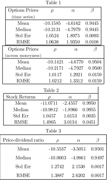
3.2.3. Simulation Results about Estimated Preference Parameters We investigate the properties of the estimators for the preference parameters while holding the other parameters of the model …xed at their true values.11 In Tables 1, 2 and 3 we report the results of this simulation experiment in terms of mean, median, standard error and root mean square error (RMSE) for the three parame-ters. We report the results for the method-of-moments estimators based on option prices (from a time series and an across-moneyness perspective), stock returns, and price-dividend ratios12respectively. First, we notice that the estimators based on stock returns are more biased than the estimators based on moment conditions for options. It is the case even if we use comparable moments computed on the time series of one particular option. The bias is more pronounced for the pa-rameters ½ and ® than for the subjective discount factor ¯: A possible reason for this …nite sample bias could be the nonlinearity in parameters present in the model.13 It is possible that the nonlinear nature of the option payo¤s helps in this regard. Improvements in terms of RMSE can be obtained in two directions, one for options, the other for the stock.
First, by using a set of three options with di¤erent moneyness, we can see that the RMSE is reduced at least for ½ and ®: The main di¤erence in the information base of the sets of estimators is that in one case we use a time series of a unique asset, while in the other we use a panel of option prices.14 To estimate well the
11The values of the endowment process are similar to those estimated from actual data by
Bonomo and Garcia (1996). Other values, such as the ones used in David and Veronesi (1999), yielded the same conclusions.
12The informational content of price-dividend ratios was suggested by Bansal and Lundblad
(1999).
13This is not a numerical issue. In fact, we gave an advantage to the stock returns conditions
in the sense that we started the optimization at the true parameter values, while for the options the initial values were taken in a random neighborhood of the true values.
14On the one hand, we use more information by having three price series, on the other hand
we do not use this information as e¢ciently since we limit ourselves to …rst moments in the estimation to obtain the three moment conditions needed to estimate ¯; ½ and ®:
preference parameters, it is necessary to recover well the stochastic discount factor or the underlying risk neutral probability distribution. This is easier with a panel of option prices than with a time series on the underlying asset or one particular option. The second direction of improvement is to use moments on the price-dividend ratio of the stock instead of stock returns to estimate the parameters. The RMSE is reduced for the three parameters compared to the estimates obtained with the stock returns. It should be emphasized that in the true model used to simulate the prices, the price-dividend ratio takes two values, one for each state, as it is the case for option prices. We therefore added noise to log('(Ut) as log('(Ut)) + ¾Y(Ut)vt where vt is an i:i:d: N(0; 1) process, in the same way we did for normalized option prices. However the RMSEs remain higher than the RMSEs obtained with option prices.
Several conclusions can be drawn from the simulation results. First, it seems fair to state that stock return data provide poor estimates of the preference para-meters. While price-dividend ratios produce better estimates, the standard errors for ½ and ® are higher than for stock returns. Moreover, the distribution of ® is dramatically skewed to the right, producing a marked underestimation in average of the risk aversion coe¢cient 1 ¡ ®: The superior inference produced by option prices is all the more remarkable that we have used not the Euler equations but the generalized Black-Scholes formula, which already incorporates the information conveyed by observed bond and stock prices, for estimating the preference para-meters. In other words, in such an exercise, option pricing formulas that are close to Hull and White preference-free formula would have led to option price data without any informational content about preference parameters. What we have captured in our estimation with moments on options is the marginal information provided by option prices in excess of the information provided by bond and stock prices.
3.2.4. Estimating all Model Parameters with Simulated Prices
In reality we cannot consider that we know any of the parameters of the model. In order to estimate simultaneously all the structural parameters of our model we combine moment conditions from the stock returns and option price series. It should be emphasized that the only observables are the stock and option price data, and the dividend series (to construct the stock returns including dividends).
The consumption series does not need to be observed. The estimation method will allow us to infer values for the means and variance of consumption growth from …nancial market data as it was done by Bonomo and Garcia (1996) using a maximum likelihood approach. We also need to compute from Euler equations, given values for the other model parameters, the price-consumption ratios ¸1and ¸2for the market portfolio and the price-dividend ratios '1 and '2for the stock. In Table 4, we proceed to estimate jointly all the parameters of the model, again with an exact method of moments applied to the simulated asset prices as above. We use enough moment conditions from option prices and stock returns to estimate the 12 parameters of interest. We get 9 moment conditions on options by considering 3 di¤erent moneynesses (1.1, 1 and 0.9) and times to maturity (1, 2 and 3 periods) and three moment conditions from the stock returns (mean, variance and covariance). At each stage of the estimation, given the current set of values for the model parameters, the ¸ and the ' parameters are computed by solving the Euler equations. The results indicate that the preference parameters, the transition probabilities and the consumption-dividend correlation parameter are estimated without bias and rather precisely. It is not the case for the means and variance of the consumption process, which are biased. The variance parameters of the dividend process are slightly biased upward.15 Acknowledging these potential problems in recovering some parameters, we will nevertheless proceed with this method for estimating the parameters of the model with actual data since it allows to recover well the preference parameters which are the main focus of our analysis.
3.3. Is There Evidence of Preference Parameters in S&P 500 Option Prices?
The simulation experiments of the last section lay the ground for a general esti-mation of the model with option price and stock return data. To estimate the parameters and assess the out-of-sample pricing performance of the various mod-els, we use daily price data for S&P 500 Index call European options obtained from the Chicago Board Options Exchange for the period January 1991 to
De-15However, it should be noted that the median bias of the estimators for the consumption and
cember 1995.16 The S&P 500 index option market is extremely liquid and it is one of the most active options markets in the United States. This market is the closest to the theoretical setting of the Black-Scholes model and the extensions proposed in this paper. We also used daily return data for the S&P 500 Index.
3.3.1. Estimation of the Parameters
We used the following method of estimation. At time t, the GBS model is esti-mated by the method of moments using the moments de…ned in the simulation study. By estimating parameters for options of di¤erent maturities and moneyness we take the model to the letter. The same preferences should apply to the pricing of all assets. Therefore, we include options of all maturities and moneyness. Also, the same preference parameters will apply to the risk premia associated with the state variable that makes the mean of the consumption process or the volatility of the dividend jump. In that sense our approach distinguishes itself from arbitrage-based methods as developed in Pan (2002), where risk premia are estimated as if investors had di¤erent risk attitudes towards the various types of risk. To com-pute the empirical moments, we use a three-month window prior to the time of estimation. This last feature also pushes in the direction of estimating the struc-tural parameters of the model. Often option pricing models are estimated with a window as short as a day making the process more like a calibrating exercise than an estimation one. We will pursue further such a calibration exercise in the next section.
More precisely, the parameters are estimated based on matching the following moments for the options:
f (St K; (T ¡ t); µ) = E · GBS µ Ut; St K; (T ¡ t) ¶¸ ¡ 1 MSt=K t X ¿=t¡h ¼¿ µ St K; (T¡ t) ¶ ; (3.9) where the expectation is with respect to Ut, h equals 3 months, and µ regroups all the parameters. The notation ¼¿(SKt; (T ¡ t)) denotes a call option on the underlying stock at time ¿ , with a moneyness equal to St=K and a maturity equal to (T ¡ t). The quantity MSt=K represents the number of options over the period 16Rosenberg and Engle (2002) use the same 1991-1995 period for estimating empirical pricing
h with a moneyness equal to St=K . We proceeded by partitioning the options into moneyness categories based on St
K and maturity categories based on (T-t). It should be noted that we take an unconditional expectation of the GBS formula to build unconditional moments.
We then minimized X X
f(St
K; (T ¡ t); µ) 2
; (3.10)
where the …rst summation is over moneyness categories and the second over the maturity categories. We also included some moment conditions based on the stock returns and conditions based on the Euler equations for the identi…cation of ¸ and ';in order to obtain as many moment conditions as there were parameters to estimate.
For the estimation, we start each trading day with a set of initial values and use …rst a simplex algorithm to obtain initial estimates followed by a DFP rou-tine17. The same strategy is also applied to the expected utility model where ° is constrained to a value of 1. We conduct this experiment for …ve years, from 1991 to 1995. Table 5 reports the average values of the preference parameters that we obtained in each of the …ve years and over the …ve-year period. Look-ing …rst at the GBS model, we can say that the estimates of the risk aversion and intertemporal substitution parameters appear reasonable. Over the …ve-year period, the coe¢cient of relative risk aversion is equal to 0.6838 on average and the elasticity of intertemporal substitution has a mean value of 0.8532. This is a result that conforms with intuition since one generally expects that the inverse of the elasticity of substitution should be greater than the coe¢cient of relative risk aversion, as emphasized in Weil (1989). As the yearly means and standard errors indicate, the values obtained are remarkably stable over time, a reassuring fact for a structural model with a representative investor. It is interesting to compare these estimates with the values obtained when we constrain the parameter ° to be equal to 1. Similarly to what was obtained with stock returns series in various studies aimed at solving the equity premium puzzle, we obtain a high average value of 7.16 for the coe¢cient of relative risk aversion, with a standard deviation of 4.83. It is interesting to note that over the same 1991-1995 period, Rosenberg
17To make sure that we explore well the parameter space in the optimization, and especially
the preference parameters, we also used a grid of initial values for the preference parameters. The …nal results were similar.
and Engle (2002) …nd an empirical risk aversion of 7.36 with a power utility func-tion de…ned over wealth (measured by the S&P 500 index), based on S&P 500 option price data. Bakshi, Kapadia and Madan (2001) also estimate by GMM the coe¢cient of relative risk aversion in a power utility setting based on a relation between the risk-neutral skewness of index returns and conditional moments of the physical index distribution. Depending on the set of instruments, estimates are in the range 1.76 to 11.39.18 Therefore, relaxing the constraint ° = 1 allows for a more reasonable value for the elasticity of intertemporal substitution. The value found for ¯ in the expected utility case is somewhat low (0.88 on average), while it appears more reasonable (0.94 average) when ° is not constrained to be equal to one.
Another way to assess the reasonableness of the model estimates for the pricing of the assets is to look at the estimates obtained for the other parameters of the model, both the fundamental processes and the state variable. The averages over the 1991-1995 period are given in Table 6. As we saw in the theoretical formulas in Section 2, the price-consumption (¸) and the price-dividend (') ratios play a fundamental role in the pricing of the assets. We found averages of around 8 and 11 for the price-consumption ratio and 13 and 19 for the price-dividend ratio with little variability over the …ve-year period (standard deviations of 0.67 and 0.85 respectively). These values also appear reasonable.
In terms of the state variable we …nd average values of 0.9758 and 0.8078 for the transition probabilities in state 1 and 2 respectively, implying values of 0.89 and 0.11 respectively for the unconditional probabilities. State 1 is in fact a crash-like state with a very negative mean for consumption growth (-0.32 on average), but one should not forget however that the state variable also controls the volatility of dividends. So state 1 is in fact a low volatility of dividends and low-consumption state. Given the negative mean value of dividends, it appears that the representa-tive investor attributes an unreasonably high probability to the bad state, while as we just saw the inferred preference parameters are reasonable. This is in contrast with the results obtained by Jackwerth (2000) with a nonparametric methodology. In a parametric framework, Rosenberg and Engle (2002) …nd results that di¤er
18However, most of the estimated values are in the neighborhood of 2. This is obtained for
short and medium-term options. It is close to the average value of 2.35 that we obtain with short-term options in section 4.
from Jackwerth (2000), in particular they do not …nd negative risk aversions when they use a power pricing kernel. Rosenberg and Engle (2002) …nd results similar to Jackwerth’s results when they use an orthogonal polynomial pricing kernel. In particular, they …nd that there is a region of negative risk aversion over the range from -4% to 2% for returns. Our estimates of the model parameters suggest that the potential mispricing comes from a very pessimistic assessment of the funda-mentals of the economy and not from unreasonable preferences.19 In any case, this exercise illustrates the di¢culty of disentangling the subjective probability assessments of the states from the preferences. In the nonparametric framework of Jackwerth (2000), the risk aversion function is recovered by treating as given both the option prices and the stock index prices to estimate non-parametrically the risk-neutral and subjective probabilities respectively and by taking their ra-tios. If prices were generated from our economy with state variables it is possible that one could recover a bimodal graph for preferences as Jackwerth (2000) does even though preferences are here constant. The values extracted for the probabil-ities, say from an implied binomial tree, are pseudo-true values (since the tree is likely to be misspeci…ed) and will depend on all the parameters of the economy, including preference parameters. Therefore, the separation between probabilities and preferences is not as obvious as it seems. Finally, the values estimated for the volatility parameters, both consumption and dividends, appear quite reasonable.
3.3.2. Pricing Errors
In this section, we will assess the pricing errors associated with our generalized non-expected utility option pricing formula and compare them with the errors ob-tained with the expected utility model and a preference-free stochastic volatility model. Using the estimates obtained each trading day following the estimation
19The unreasonable parameters for the fundamentals process may also result from a
misspec-i…cation of the growth rate equations.We could increase the number of states as in Bonomo and Garcia (1996) where a three-state bivariate Markov switching model is estimated on an annual frequency over the last century or so. It should also be noted that our state variable captures both the jump and the stochastic volatility e¤ects. A way to disentangle the two would be to introduce a GARCH speci…cation in the volatility of dividends.
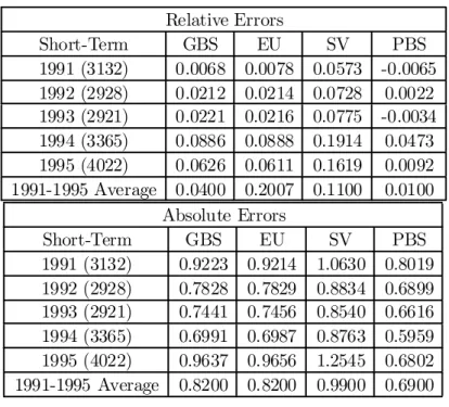
method described in the previous section20, we forecast the prices for all the options of the following day separated in long (more than 180 days), medium (between 180 and 60 days) and short (less than 60 days) maturities irrespective of moneyness. We average the daily forecast errors over each year for the cor-responding categories and compare the performance with the absolute and the relative errors for various maturity categories for all three models. Christo¤ersen and Jacobs (2001) have recently emphasized that the loss function used in para-meter estimation and model evaluation should be the same. We use an absolute dollar measure which is consistent with the mean square criterion used in estima-tion, but we add also a relative measure to give an idea of the magnitude of the error. The results are shown in Table 7. The absolute errors appear to be roughly uniform across maturities, but the relative loss is much smaller for the expensive long-term options than for the cheap short-term options. However, the ranking of the models is the same for both measures.
We compare three models: the most general option model for the non-separable recursive utility model given by formula (2.21), the expected utility model ob-tained by setting ° equal to one in (2.21) to judge the importance of non-separabilities, and …nally the preference-free stochastic volatility model which results from (2.21) when QXY(t; T ) = 1 to gauge the importance of preferences for option prices. It should be emphasized that the objective of this forecasting exercise is to assess the relative performance of the three models. One cannot hope to obtain errors of small magnitude by using only unconditional moments in the estimation and a rather long window in the past. Conditional information needs to be incorporated in some way to achieve more sensible pricing performances. This can be done in a structural way by using the option pricing formula as a function of the unobserved state and by …ltering the current value of the latent state variable. We will take a simpler approach in the next section by incorporating conditioning information such as BS implied volatilities in an ad-hoc way in the model.
The results are clear. For all maturities, GBS does better that the speci…cation where ° is equal to one which in turn is better than the SV speci…cation.21
Com-20The parameters for the stochastic volatility model are estimated with the same moment
conditions as the two preference models but we impose the constraint that QXY(t; T ) is equal
to one.
pared to the stochastic volatility model, the relative error for GBS is reduced by up to 50 per cent for short-term and medium-term options. This shows that pref-erences are important in pricing options on the index. Moreover, the data seem to indicate that preferences are of the non-separable type since the restricted value of ° generally increases the relative error. Of course, as we advance in maturity, the relative error falls for all models since the volatility smile ‡attens and pric-ing tends to approach Black-Scholes. However, for long-term options, the GBS model performs signi…cantly better than the other two. These results parallel the simulation results reported in Garcia, Luger and Renault (2001) about the smile e¤ect. First, it was shown that a non-preference free framework was able to re-produce the various asymmetries observed in the implied volatility curve inferred from option price data. Second, the parameter ° was seen to be more important than the risk aversion parameter ® in calibrating the smile.
To conclude this section, it seems fair to say that we have obtained reasonable values of the preference parameters based on price data of all options, irrespective of their moneyness and maturity, but that the pricing errors are very large. In the next section, we take some liberty with the model and show that by incorpo-rating conditioning information, focussing on short-term options speci…cally and reducing the estimation window, the pricing errors are reduced considerably.
4. Calibrating the Model for Practical Option Pricing
In the last section, the goal was to obtain estimates of the structural parameters of the model. In this section, we aim at minimizing the out-of-sample pricing errors in the spirit of Bakshi, Cao and Chen (1997). In this type of exercise one typically makes concessions with the structural model. The window for estimating the parameters is generally very short (from a day to a week) and conditioning information is included in an ad hoc way, usually inconsistent with the model. The best example of this ad hoc approach is to use the BS formula to extract implied volatility on a given day for a certain maturity and moneyness and to use this volatility to price options the next day with the same maturity and moneyness. In so doing, practitioners completely ignore the fact that the assumption of constant most papers in the literature, but tests of predictive accuracy (as in Diebold and Mariano, 1995 or West, 1996) could be applied (see Dumas, Fleming and Whaley, 1998).
volatility underlying the BS model is obviously violated since the implied volatility may vary widely from one day to the next. Yet they use the formula as a tool and the performance of this rather crude method is di¢cult to beat by more sophisticated models unless one is ready to recognize that the parameters of the model are unstable and their estimates need to be updated.22
In what follows, we have decided to adapt our model in an ad hoc way in order to improve its out-of-sample pricing performance. First, we reduce the window over which we estimate the parameters to 5 days instead of 3 months. Second, we incorporate the option’s implied volatility ¾¤
t into the dividend volatility process as23:
¾Y(Ut= j) = ±0j + ±1j¾¤t p
(T ¡ t); (4.1)
for j = 1; 2.
Parameter estimates were then based on a modi…cation of the estimation method where, for a given maturity (T-t), we minimized
1 MSt=K t X ¿ =t¡h · E · GBS µ Ut; St K; (T ¡ t); ¾ ¤ t ¶¸ ¡ ¼¿ µ St K; (T¡ t) ¶¸2 : (4.2)
Note that we maintain the use of unconditional moments.24 Therefore, there is a di¤erent set of parameter estimates for each maturity category. (This relaxes the implicit constraints of the form p(2)
ik = p (1) ij p (1) jk, where p (s)
¢¢ are s-period transition
22Heston and Nandi (2000) claim that their closed-form GARCH option pricing formula
out-perform the ad hoc BS model of Dumas, Fleming and Whaley (1998) even without updating but a closer look at the results (Table 7) shows that this is not true for short-term options. Even with updating the GARCH model does not outperform the ad hoc BS approach for close-to-the-money short-term options. Moreover, a more precise procedure, using a model estimated with the same criterion as in the out-of-sample performance evaluation, produces a smaller error for the practitioner Black-Scholes methodology, as pointed out by Christo¤ersen and Jacobs (2001).
23ThepT¡ t in the formula below refers to the exact maturity of each option used to extract
the corresponding implied volatility.
24We could have probably improve further the out-of-sample pricing performance by …ltering
the state probability at time t and use this information to compute the expectation of the GBS formula.
probabilities). Also, we now leave aside the moment conditions based on stock returns and use only the moment conditions associated with the options.
In addition, we impose the following constraints:
Et[QXY(t; T )] = 1; (4.3)
Et[ eB(t; T )] = exp(¡r(T ¡ t)); (4.4) where r is the observed interest rate. These constraints were implicitly embodied in the original estimation method in section 3 through the Euler equations for ¸ and '. With the modi…ed method, it is no longer (numerically) feasible to enter the Euler equations into the estimation problem since ' depends on ¾Y, which now depends on ¾¤
t. Therefore, ¸ and ' are treated as free parameters to be explicitly estimated along with the other model parameters; hence the …rst constraint. The second constraint serves to incorporate information on the interest rate.
Let us start with pricing errors since the goal of the calibration exercise is to improve the out-of-sample performance. We now use estimates obtained every day to forecast the prices for all the short maturity (less than 60 days) options of the next day irrespective of moneyness. We average the daily forecast errors over each year and compare the performance of the previous three models (non-expected utility, (non-expected-utility and preference-free stochastic volatility) to which we added a practitioner BS model in the spirit of Dumas, Fleming and Whaley (1998).25 Table 8A reports the absolute and relative pricing errors for each year in the 1991-1995 period. First, note that the relative errors associated with the preference-based GBS or EU formulas have fallen considerably and vary between 1% and 9%. It is interesting to note that the two preference-based models produce now very similar errors. However, the relative errors of the BS ad hoc model remain smaller. We also report in Table 8B out-of-sample pricing errors at a horizon of 5 days for the GBS and PBS models. The gap between the two models
25Note that we do not estimate a volatility function as in Dumas, Fleming and Whaley (1998).
We simply group options by moneyness categories and forecast the volatility of an option one day ahead by the implied volatility of the moneyness category the day before. The procedure of Christo¤ersen and Jacobs (2001) might have produced a lower error for the practitioners’ BS model.
is mostly maintained, except in the beginning of the sample where the BS absolute error tends to increase faster than the GBS one.26
The reduction in pricing errors with respect to section 3 can come from three sources. We assess the contribution of each source for the year 1991. First, in this calibration exercise, we focus the estimation on short-term options, compared with all options in section 3. Reestimating the same GBS model only for short options reduces by half the absolute error for the year 1991 (from 3.14 to 1.52 for the absolute error and from 0.859 to 0.285 for the relative error). The second source of error reduction is the reduced span of the data to carry out the estimation, from three months to 5 days. This brings down the absolute error to 1.41 and the relative error to 0.0935, but these are still higher than the highest errors of Table 8A for the SV model. Indeed, the introduction of the implied volatility information reduces substantially the errors, bringing down the absolute error to 0.92 and the relative error to 0.0068 as reported in Table 8A.
The errors of the SV model are de…nitely higher than the ones of the PBS model yet they both use implied volatility. The main di¤erence comes from the fact that the PBS method uses the implied volatility of the day before while the SV method smoothes the implied volatility of the last …ve days. This underlines the penalty imposed by the averaging over the past values for out-of-sample forecasting. The risk aversion parameter appears therefore of prime importance since it reduces the error considerably despite the averaging e¤ect over …ve days for the implied volatility.
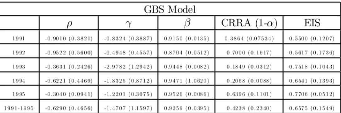
A reassuring result is that the preference parameter estimates obtained for the GBS model, although much more variable than before both within and between the years, are close to the estimates we obtained with the 3-month window esti-mation, as illustrated in Table 9. Both the relative risk aversion coe¢cient and the elasticity of intertemporal substitution are slightly lower on average (0.42 and 0.66 respectively). The risk aversion parameter in the expected utility model is now estimated at a lower more reasonable value of 2.35. Notice also that the estimates of ¯ in the expected utility model are much more reasonable than with the previous method both for the EU and the GBS models. While the parameters are di¢cult to interpret in this less structural model, it is worth noting that
26As expected, this trend is even more accentuated for longer horizons such as t+10 and t+15.
we obtained more reasonable parameters for the consumption mean parameters (1% and -17% in states 1 and 2, where state 1 is also the low dividend volatility parameter, and where p11 and p22 are 0.80 and 0.22 respectively. Therefore, the good state (high level of consumption growth and low volatility of dividends27) appears to be more frequent as one should expect.
5. Conclusion
In this paper, we contribute to the empirical asset pricing literature by estimating a recursive utility model with option prices. Not only do we show that preferences matter for option pricing but also that option prices help distinguish between the expected and the non-expected utility models. The informativeness of option price data about preference parameters is con…rmed in a simulation experiment. The estimates we obtain for the preference parameters are quite reasonable. This is in contrast with recent results of Jackwerth (2000) who infers risk aversion functions that are at odds with usual theoretical assumptions. It should be emphasized that in our method preference parameters enter consistently in the equilibrium pricing of all assets.
Of course, given the simplicity of the practitioners’ Black-Scholes approach and its good predictive performance, our structural model faces a tough challenge as a competitor. However, we consider that both our simulation experiments and the estimation performed with S&P 500 option price data strongly support the claim that preference parameters are important in option pricing. To better understand the structure of index option prices, one can think of several possible extensions in terms of preference speci…cations or distributions for the state variables. One potential weakness of our model for fundamentals is the modeling of volatility. Our speci…cation captures only sudden changes in volatility in dividends. The model will gain by adding some GARCH e¤ects to the switching regimes governing the dividend process.
27This is in line with usual empirical evidence. It is hard to say what explains the changes
in parameters estimates with respect to the unintuitive results obtained in section 3.3.1 where options of all maturities and moneyness were considered all together.
The paper was presented at the Conference on Risk Neutral and Objective Probabilities at Duke University in October 2000, the WFA 2001 in Tucson, the ESC-IDEI Conference (Toulouse) and the CIRANO-CRM Workshop (Montréal), as well as at Boston College, the Fields Institute (University of Toronto), McGill University, the University of Chicago, and the University of Rochester. The authors thank F. Bandi, C. Jones, C. Lundblad and L. P. Hansen, two anony-mous referees and the editors for their helpful comments and suggestions, and conference and seminar participants. The …rst two authors gratefully acknowledge …nancial support from the Fonds de la Formation de Chercheurs et l’Aide à la Recherche du Québec (FCAR), the Social Sciences and Humanities Research Council of Canada (SSHRC) and the MITACS Network of Centres of Excellence. The third author thanks CIRANO, C.R.D.E. and IFM2 for …nancial support. This paper represents the views of the authors and does not necessarily re‡ect those of the Bank of Canada or its sta¤.
References
[1] Aït-Sahalia, Y., and A.W. Lo, 2000, Nonparametric Risk Management and Implied Risk Aversion, Journal of Econometrics 94, 9-51
[2] Amin, K.I. and V.K. Ng, 1993, Option Valuation with Systematic Stochastic Volatility, Journal of Finance 48, 3, 881-909.
[3] Amin, K.I. and R. Jarrow, 1992, Pricing Options in a Stochastic Interest Rate Economy, Mathematical Finance, 3(3), 1-21.
[4] Bakshi, G., Kapadia, N., and Madan, D., 2001, Stock Return Characteristics, Skew Laws, and Di¤erential Pricing of Individual Equity Options, Review of Financial Studies, forthcoming.
[5] Bakshi, G., C. Cao and Z. Chen, 1997, Empirical Performance of Alternative Option Pricing Models, Journal of Finance 94, 1-2, 277-318.
[6] Bansal, R. and C. Lundblad, 1999, Fundamental Values and Asset Returns in Global Equity Markets, Working Paper, Duke University.
[7] Bates, D., 1996, Testing Option Pricing Models, in: Maddala and Rao, eds, Handbook of Statistics, Vol. 14: Statistical Methods in Finance, 567-611. [8] Bates, D., 2000, Post-’87 Crash Fears in the S&P 500 Futures Option Market,
Journal of Econometrics, 94, 181-239.
[9] Black, F. and M. Scholes, 1973, The Pricing of Options and Corporate Lia-bilities, Journal of Political Economy 81, 637-659.
[10] Bonomo M. and R. Garcia, 1994a, Can a Well-Fitted Equilibrium Asset Pric-ing Model Produce Mean Reversion?, Journal of Applied Econometrics 9, 19-29.
[11] Bonomo M. and R. Garcia, 1994b, Disappointment Aversion as a Solution to the Equity Premium and the Risk-Free Rate Puzzles, CIRANO working paper 94s-14.
[12] Bonomo, M. and R. Garcia, 1996, Consumption and Equilibrium Asset Pric-ing: An empirical Assessment, Journal of Empirical Finance 3, 239-265.